
A Generative Adversarial Network Structure for Learning with Small Numerical Data Sets


Abstract
:1. Introduction
2. Literature Review
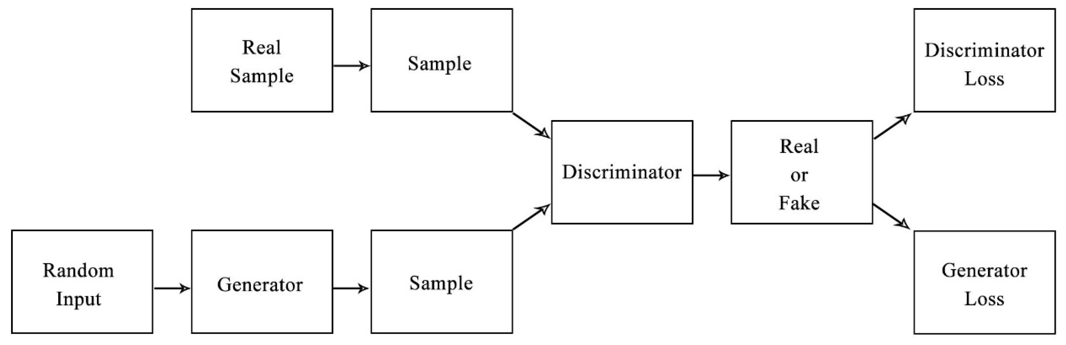
2.1. The Generative Adversarial Networks
2.2. Information Diffusion
2.3. The Mega-Trend-Diffusion
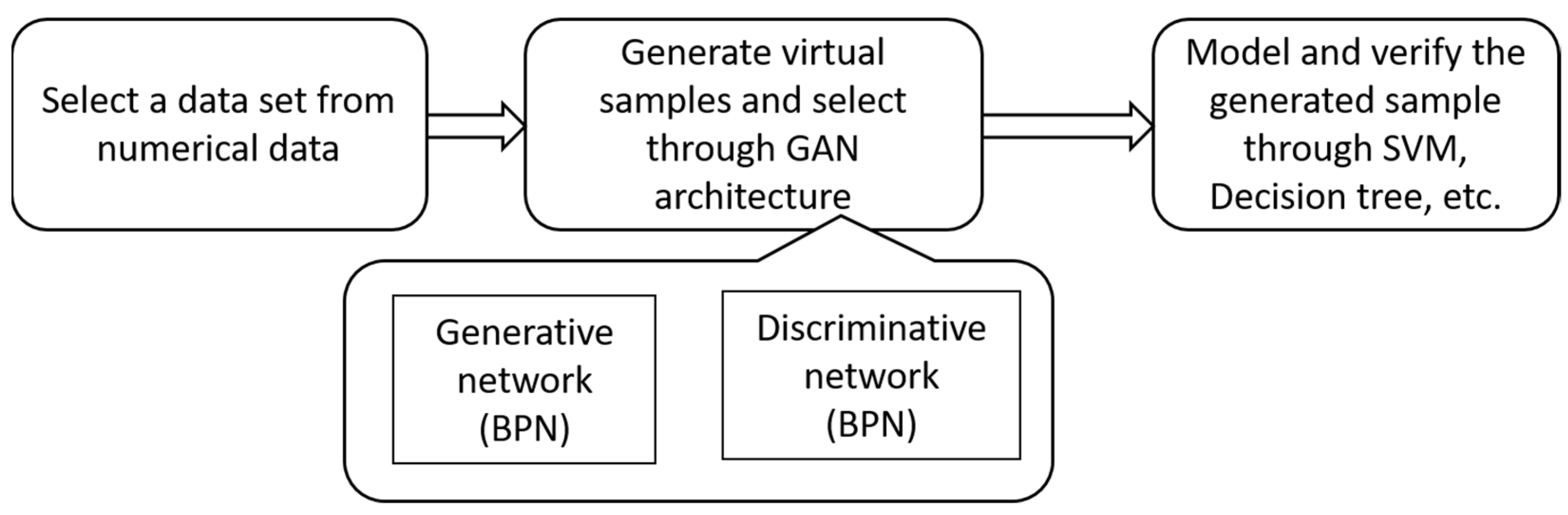
3. Methodology
3.1. Virtual Sample Generation and Selection
3.1.1. The Architecture of WGAN_MTD
3.1.2. Training Steps for WGAN_MTD
3.1.3. MTD in Range Estimation
3.1.4. The Process of Sample Generation with WGAN_MTD
4. Experimental Study
4.1. Evaluation Criterion
4.2. Experiment Environment and Datasets
4.3. Experiment Results
5. Conclusions
Author Contributions
Funding
Institutional Review Board Statement
Informed Consent Statement
Data Availability Statement
Conflicts of Interest
References
- Ivǎnescu, V.C.; Bertrand, J.W.M.; Fransoo, J.C.; Kleijnen, J.P.C. Bootstrapping to solve the limited data problem in production control: An application in batch process industries. J. Oper. Res. Soc. 2006, 57, 2–9. [Google Scholar] [CrossRef] [Green Version]
- Kuo, Y.; Yang, T.; Peters, B.A.; Chang, I. Simulation metamodel development using uniform design and neural networks for automated material handling systems in semiconductor wafer fabrication. Simul. Model. Pract. Theory 2007, 15, 1002–1015. [Google Scholar] [CrossRef]
- Lanouette, R.; Thibault, J.; Valade, J.L. Process modeling with neural networks using small experimental datasets. Comput. Chem. Eng. 1999, 23, 1167–1176. [Google Scholar] [CrossRef]
- Oniśko, A.; Druzdzel, M.J.; Wasyluk, H. Learning Bayesian network parameters from small data sets: Application of Noisy-OR gates. Int. J. Approx. Reason. 2001, 27, 165–182. [Google Scholar] [CrossRef] [Green Version]
- Chao, G.Y.; Tsai, T.I.; Lu, T.J.; Hsu, H.C.; Bao, B.Y.; Wu, W.Y.; Lin, M.T.; Lu, T.L. A new approach to prediction of radiotherapy of bladder cancer cells in small dataset analysis. Expert Syst. Appl. 2011, 38, 7963–7969. [Google Scholar] [CrossRef]
- Huang, C.J.; Wang, H.F.; Chiu, H.J.; Lan, T.H.; Hu, T.M.; Loh, E.W. Prediction of the period of psychotic episode in individual schizophrenics by simulation-data construction approach. J. Med Syst. 2010, 34, 799–808. [Google Scholar] [CrossRef]
- Li, D.C.; Lin, W.K.; Chen, C.C.; Chen, H.Y.; Lin, L.S. Rebuilding sample distributions for small dataset learning. Decis. Support Syst. 2018, 105, 66–76. [Google Scholar] [CrossRef]
- Liu, Y.; Zhou, Y.; Liu, X.; Dong, F.; Wang, C.; Wang, Z. Wasserstein GAN-Based Small-Sample Augmentation for New-Generation Artificial Intelligence: A Case Study of Cancer-Staging Data in Biology. Engineering 2019, 5, 156–163. [Google Scholar] [CrossRef]
- Gonzalez-Abril, L.; Angulo, C.; Ortega, J.A.; Lopez-Guerra, J.L. Generative Adversarial Networks for Anonymized Healthcare of Lung Cancer Patients. Electronics 2021, 10, 2220. [Google Scholar] [CrossRef]
- Ali-Gombe, A.; Elyan, E. MFC-GAN: Class-imbalanced dataset classification using multiple fake class generative adversarial network. Neurocomputing 2019, 361, 212–221. [Google Scholar] [CrossRef]
- Shamsolmoali, P.; Zareapoor, M.; Shen, L.; Sadka, A.H.; Yang, J. Imbalanced data learning by minority class augmentation using capsule adversarial networks. Neurocomputing 2021, 459, 481–493. [Google Scholar] [CrossRef]
- Vuttipittayamongkol, P.; Elyan, E. Improved overlap-based undersampling for imbalanced dataset classification with application to epilepsy and parkinson’s disease. Int. J. Neural Syst. 2020, 30, 2050043. [Google Scholar] [CrossRef]
- Goodfellow, I.; Pouget-Abadie, J.; Mirza, M.; Xu, B.; Warde-Farley, D.; Ozair, S.; Courville, A.; Bengio, Y. Generative adversarial nets. Adv. Neural Inf. Process. Syst. 2014, 27, 2672–2680. [Google Scholar]
- Efron, B.; Tibshirani, R.J. An Introduction to the Bootstrap; CRC Press: New York, NY, USA, 1994. [Google Scholar]
- Niyogi, P.; Girosi, F.; Poggio, T. Incorporating prior information in machine learning by creating virtual examples. Proc. IEEE 1998, 86, 2196–2208. [Google Scholar] [CrossRef] [Green Version]
- Li, D.C.; Chen, L.S.; Lin, Y.S. Using functional virtual population as assistance to learn scheduling knowledge in dynamic manufacturing environments. Int. J. Prod. Res. 2003, 41, 4011–4024. [Google Scholar] [CrossRef]
- Huang, C.F. Principle of information diffusion. Fuzzy Sets Syst. 1997, 91, 69–90. [Google Scholar]
- Huang, C.; Moraga, C. A diffusion-neural-network for learning from small samples. Int. J. Approx. Reason. 2004, 35, 137–161. [Google Scholar] [CrossRef] [Green Version]
- Li, D.C.; Lin, W.K.; Lin, L.S.; Chen, C.C.; Huang, W.T. The attribute-trend-similarity method to improve learning performance for small datasets. Int. J. Prod. Res. 2016, 55, 1898–1913. [Google Scholar] [CrossRef]
- Mirza, M.; Osindero, S. Conditional generative adversarial nets. arXiv 2014, arXiv:1411.1784. [Google Scholar]
- Arjovsky, M.; Chintala, S.; Bottou, L. Wasserstein Generative Adversarial Networks. arXiv 2017, arXiv:1701.07875. [Google Scholar]
- Yamashita, R.; Nishio, M.; Do, R.K.G.; Togashi, K. Convolutional neural networks: An overview and application in radiology. Insights Imaging 2018, 9, 611–629. [Google Scholar] [CrossRef] [PubMed] [Green Version]
- Li, D.C.; Wu, C.S.; Tsai, T.I.; Lina, Y.S. Using mega-trend-diffusion and artificial samples in small data set learning for early flexible manufacturing system scheduling knowledge. Comput. Oper. Res. 2007, 34, 966–982. [Google Scholar] [CrossRef]


| Datasets | Total Samples | Input Attributes | Output Attributes | Number of Samples | ||
|---|---|---|---|---|---|---|
| Class 1 | Class 2 | Class 3 | ||||
| Wine | 178 | 13 | 1 | 59 | 71 | 48 |
| Seeds | 210 | 6 | 1 | 70 | 70 | 70 |
| Cervical Cancer | 72 | 18 | 1 | 21 | 51 | - |
| SVM_Poly | SVM_Rbf | Decision_Tree | Naive_Bayes | |||||
|---|---|---|---|---|---|---|---|---|
| SDS | PM | SDS | PM | SDS | PM | SDS | PM | |
| 1 | 58.333% | 59.524% | 66.071% | 91.071% | 61.310% | 75.000% | 59.524% | 70.833% |
| 2 | 64.286% | 7H.571% | 89.881% | 86.905% | 75.000% | 85.119% | 68.452% | 82.143% |
| 3 | 83.929% | 90.476% | 92.262% | 92.857% | 81.548% | 75.595% | 89.881% | 87.500% |
| 4 | 73.214% | 85.119% | 73.810% | 91.667% | 49.405% | 46.429% | 51.786% | 47.024% |
| 5 | 62.500% | 95.833% | 76.190% | 77.976% | 55.952% | 76.190% | 68.452% | 71.429% |
| 6 | 61.905% | 76.190% | 83.333% | 92.262% | 75.595% | 83.929% | 62.500% | 73.810% |
| 7 | 77.515% | 89.349% | 85.799% | 84.024% | 73.373% | 82.840% | 59.763% | 72.189% |
| 8 | 67.456% | 65.089% | 81.065% | 83.432% | 66.272% | 64.497% | 26.036% | 60.947% |
| 9 | 77.381% | 80.357% | 79.762% | 77.976% | 63.690% | 72.619% | 58.333% | 58.333% |
| 10 | 57.738% | 69.643% | 79.167% | 86.905% | 75.595% | 70.833% | 59.524% | 72.024% |
| 11 | 63.095% | 75.000% | 85.714% | 88.095% | 67.262% | 58.929% | 58.333% | 73.810% |
| 12 | 73.810% | 88.095% | 83.929% | 91.667% | 63.095% | 69.048% | 69.643% | 67.262% |
| 13 | 59.524% | 71.429% | 77.976% | 77.381% | 70.833% | 63.690% | 73.810% | 77.381% |
| 14 | 54.762% | 88.690% | 66.071% | 94.643% | 62.500% | 68.452% | 54.167% | 75.595% |
| 15 | 83.333% | 88.095% | 91.071% | 90.476% | 78.571% | 80.357% | 74.405% | 76.190% |
| 16 | 68.824% | 81.176% | 83.529% | 87.647% | 71.176% | 68.824% | 71.176% | 67.059% |
| 17 | 59.763% | 59.172% | 63.314% | 86.982% | 81.657% | 82.249% | 76.331% | 70.414% |
| 18 | 71.429% | 89.286% | 93.452% | 93.452% | 70.833% | 72.619% | 82.143% | 87.500% |
| 19 | 52.071% | 69.822% | 85.799% | 86.982% | 78.698% | 80.473% | 90.533% | 92.308% |
| 20 | 83.333% | 92.857% | 93.452% | 90.476% | 66.667% | 85.714% | 69.643% | 82.738% |
| 21 | 76.190% | 90.476% | 83.333% | 95.833% | 70.238% | 88.095% | 78.571% | 89.286% |
| 22 | 58.929% | 57.143% | 57.143% | 78.571% | 66.071% | 57.738% | 73.214% | 83.333% |
| 23 | 61.310% | 82.143% | 80.357% | 89.881% | 63.095% | 62.500% | 47.619% | 53.571% |
| 24 | 78.698% | 82.249% | 85.799% | 80.473% | 62.722% | 76.923% | 66.272% | 71.598% |
| 25 | 82.738% | 83.333% | 95.238% | 86.905% | 72.619% | 82.143% | 64.881% | 61.905% |
| 26 | 85.119% | 88.690% | 83.929% | 89.881% | 53.571% | 68.452% | 72.024% | 82.738% |
| 27 | 57.059% | 73.529% | 76.471% | 82.353% | 52.353% | 67.059% | 58.824% | 57.059% |
| 28 | 58.580% | 62.722% | 84.615% | 92.308% | 59.172% | 63.314% | 66.864% | 75.740% |
| 29 | 86.310% | 83.333% | 91.667% | 92.262% | 56.548% | 67.262% | 77.381% | 76.786% |
| 30 | 63.095% | 63.690% | 80.357% | 88.095% | 67.857% | 78.571% | 61.905% | 77.976% |
| average | 68.741% | 78.703% | 81.685% | 87.648% | 67.109% | 72.515% | 66.400% | 73.216% |
| Stddev | 10.536% | 11.189% | 9.278% | 5.250% | 8.610% | 9.720% | 12.741% | 10.822% |
| p-value | *** | ** | ** | *** | ||||
| Wine | SVM_Poly | SVM_Rbf | Decision_Tree | Naive_Bayes | |||||
|---|---|---|---|---|---|---|---|---|---|
| SDS | PM | SDS | PM | SDS | PM | SDS | PM | ||
| 10 with 100 virtual samples | average | 68.741% | 78.703% | 81.685% | 87.648% | 67.109% | 72.515% | 66.400% | 73.216% |
| Stddev | 10.536% | 11.189% | 9.278% | 5.250% | 8.610% | 9.720% | 12.741% | 10.822% | |
| p-value | *** | ** | ** | *** | |||||
| 15 with 100 virtual samples | average | 73.159% | 82.108% | 92.584% | 92.077% | 74.849% | 79.707% | 85.165% | 86.309% |
| Stddev | 9.384% | 9.739% | 3.782% | 3.546% | 7.683% | 4.691% | 8.327% | 7.292 | |
| p-value | *** | ns | ** | ns | |||||
| 20 with 100 virtual samples | average | 78.679% | 88.526% | 94.069% | 93.775% | 78.531% | 83.132% | 89.870% | 86.309% |
| Stddev | 7.410% | 6.981% | 2.639% | 2.460% | 6.229% | 3.872% | 6.169% | 4.532% | |
| p-value | *** | ns | *** | ns | |||||
| Seeds | SVM_Poly | SVM_Rbf | Decision_Tree | Naive_Bayes | |||||
|---|---|---|---|---|---|---|---|---|---|
| SDS | PM | SDS | PM | SDS | PM | SDS | PM | ||
| 10 with 100 virtual samples | average | 69.403% | 74.532% | 83.527% | 85.720% | 79.797% | 79.180% | 71.895% | 74.907% |
| Stddev | 9.701% | 8.647% | 7.425% | 5.887% | 10.215% | 8.615% | 11.355% | 10.893% | |
| p-value | * | ns | ns | * | |||||
| 15 with 100 virtual samples | average | 72.785% | 80.171% | 87.303% | 87.711% | 82.018% | 82.191% | 81.837% | 82.328% |
| Stddev | 8.595% | 7.638% | 3.820% | 3.616% | 6.461% | 5.002% | 6.949% | 6.801% | |
| p-value | *** | ns | ns | ns | |||||
| 20 with 100 virtual samples | average | 76.789% | 81.981% | 88.762% | 89.563% | 84.705% | 85.561% | 86.004% | 85.372% |
| Stddev | 8.024% | 5.940% | 3.159% | 2.531% | 3.668% | 3.297% | 3.791% | 5.074% | |
| p-value | ** | ns | ns | ns | |||||
| Seeds | SVM_Poly | SVM_Rbf | Decision_Tree | Naive_Bayes | |||||
|---|---|---|---|---|---|---|---|---|---|
| SDS | PM | SDS | PM | SDS | PM | SDS | PM | ||
| 10 with 100 virtual samples | average | 70.593% | 75.391% | 84.771% | 84.953% | 73.184% | 76.453% | 70.462% | 72.682% |
| Stddev | 8.443% | 9.056% | 8.625% | 5.982% | 9.110% | 8.107% | 10.769% | 9.997% | |
| p-value | * | * | ns | * | |||||
| 15 with 100 virtual samples | average | 74.963% | 81.224% | 86.921% | 88.761% | 80.253% | 81.741% | 79.937% | 81.592% |
| Stddev | 8.102% | 9.857% | 3.960% | 3.773% | 7.032% | 6.351% | 7.043% | 6.980% | |
| p-value | *** | * | ns | * | |||||
| 20 with 100 virtual samples | average | 75.971% | 82.891% | 87.267% | 88.938% | 83.535% | 86.171% | 80.922% | 82.782% |
| Stddev | 8.421% | 7.453% | 4.005% | 3.361% | 4.899% | 4.367% | 4.98% | 6.754% | |
| p-value | ** | * | ns | ns | |||||
| Learning Accuracy from SVM | Wine | Seeds | Cervical Cancer |
|---|---|---|---|
| MTD | 73.267% | 76.443% | 69.861% |
| WGAN | 63.748% | 61.086% | 67.218% |
| WGAN_MTD | 88.526% | 81.981% | 82.891% |
Publisher’s Note: MDPI stays neutral with regard to jurisdictional claims in published maps and institutional affiliations. |
© 2021 by the authors. Licensee MDPI, Basel, Switzerland. This article is an open access article distributed under the terms and conditions of the Creative Commons Attribution (CC BY) license (https://creativecommons.org/licenses/by/4.0/).
Share and Cite
Li, D.-C.; Chen, S.-C.; Lin, Y.-S.; Huang, K.-C. A Generative Adversarial Network Structure for Learning with Small Numerical Data Sets. Appl. Sci. 2021, 11, 10823. https://doi.org/10.3390/app112210823
Li D-C, Chen S-C, Lin Y-S, Huang K-C. A Generative Adversarial Network Structure for Learning with Small Numerical Data Sets. Applied Sciences. 2021; 11(22):10823. https://doi.org/10.3390/app112210823
Chicago/Turabian StyleLi, Der-Chiang, Szu-Chou Chen, Yao-San Lin, and Kuan-Cheng Huang. 2021. "A Generative Adversarial Network Structure for Learning with Small Numerical Data Sets" Applied Sciences 11, no. 22: 10823. https://doi.org/10.3390/app112210823
APA StyleLi, D.-C., Chen, S.-C., Lin, Y.-S., & Huang, K.-C. (2021). A Generative Adversarial Network Structure for Learning with Small Numerical Data Sets. Applied Sciences, 11(22), 10823. https://doi.org/10.3390/app112210823