A Generative Adversarial Network Structure for Learning with Small Numerical Data Sets

Abstract

In recent years, generative adversarial networks (GANs) have been proposed to generate simulated images, and some works of literature have applied GAN to the analysis of numerical data in many fields, such as the prediction of building energy consumption and the prediction and identification of liver cancer stages. However, these studies are based on sufficient data volume. In the current era of globalization, the demand for rapid decision-making is increasing, but the data available in a short period of time is scarce. As a result, machine learning may not provide precise results. Obtaining more information from a small number of samples has become an important issue. Therefore, this study aimed to modify the generative adversarial network structure for learning with small numerical datasets, starting with the Wasserstein GAN (WGAN) as the GAN architecture, and using mega-trend-diffusion (MTD) to limit the bound of virtual samples that the GAN generates. The model verification of our proposed structure was conducted with two datasets in the UC Irvine Machine Learning Repository, and the performance was evaluated using three criteria: accuracy, standard deviation, and p-value. The experiment result shows that, using this improved GAN architecture (WGAN_MTD), small sample data can also be used to generate virtual samples that are similar to real samples through GAN.

1. Introduction

An increasing number of machine learning algorithms have recently moved from academia to commercial applications. When applied to business, the number of samples collected is often small due to the need for rapid decision-making. The small-sample problem occurs in actual cases, such as in manufacturing industries [1,2,3,4], disease diagnosis [5,6,7,8], and DNA analysis of cancer patients [9]. Datasets with imbalanced classes can be regarded as another case of the small sample problem, in which learning models ignore the information from the minority, and may thus output biased results [10,11,12]. Therefore, it is a very important issue to enable machine learning to undertake effective training with a small dataset.

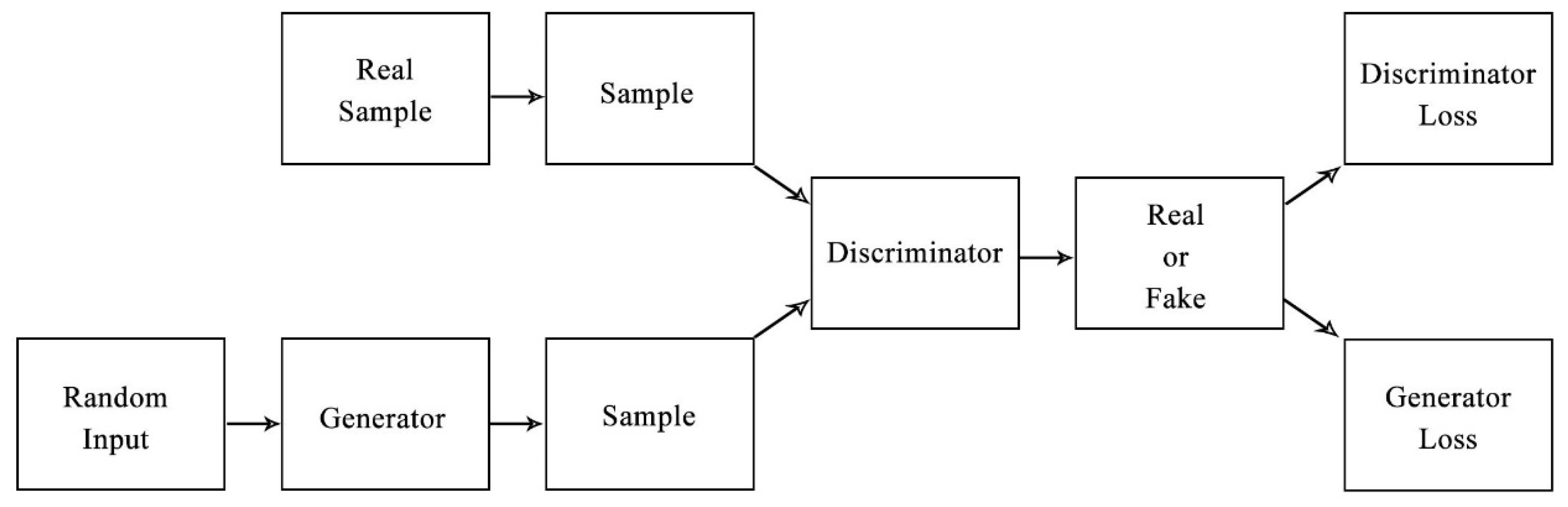
To address this issue, the main solution for the small sample problem is virtual sample generation (VSG). In recent studies, generative adversarial networks (GANs) which were proposed by Goodfellow et al. [13], have been a popular method of VSG. This approach consists of two parts—a generator and a discriminator—as shown in Figure 1. The generator is used to generate new data with a distribution similar to that of the original real data, so that the discriminator is unable to distinguish between the original and generated data, but attempts to distinguish between the two sets of data.

Typically, in statistics, a small sample can be referred to a data set with a sample size of less than 30. However, in real-world problems, the sample size should be determined according to the purpose of the survey. Because a small sample may be a tiny subset of the population, it is not possible to fully express the whole information of the population, which may lead to biased machine learning results and poor prediction performance. Furthermore, an incomplete data structure or imbalanced dataset is also a common problem in small-sample learning. It is believed that small samples still contain the underlying information. Thus, finding the clue hidden inside small samples, and inferring these samples’ corresponding population information, is meaningful for practical needs.

There are many acceptable methods for small-sample learning, of which virtual sample generation (VSG) is one of the main methods as used, for example, by Efron et al. [14] with the bootstrap method. Niyogi et al. [15], based on statistical inference mechanisms and using the principle of repeated sampling without replacement, investigated mathematical algorithms for converting limited 2D images into 3D images. Li et al. [16] produced a functional virtual population through the trial-and-error method. According to Huang [17], in order to solve the problem of incomplete information, the principle of information diffusion on display based on fuzzy theory has a more sufficient and long-term continuity and development. Huang and Moraga [18] reasoned that the normal diffusion function infers that each sample point can spread on both sides of two derivative samples, increasing the possibility of improving the accuracy of the neurologic network for learning with a small sample; this approach is called a diffusion neural network. Like the approach of Li et al. [19], based on the sample derivation formula of Huang and Moraga [18], the mega-trend-diffusion (MTD) technique takes into account the overall information of all data, and is proposed to infer the value domain of the parent.

Generative adversarial networks (GANs) have become one of the commonly used models for producing virtual samples. The GAN structure is a sample generation method developed by Goodfellow et al. [13] that uses the confrontation between the generative network (the Generator), and the discriminative network (the Discriminator) as the main core to ensure the generated virtual samples are closer to the training samples. Since the GAN method was published in 2014, it has been regarded as an important method for virtual sample generation of image data. It has also been extensively applied, and many extensions to and improvements of GANs have been made. According to the GAN Zoo website, there are more than 70 types of GAN. Mirza and Osindero [20] improved the GAN and proposed conditional generative adversarial nets (cGAN), adding additional conditions to the generative and discriminative networks, so that the model can be generated and determined with additional conditions. The improvement also transformed the GAN structure from an unsupervised learning model to a supervised model. Arjovsky et al. [21] proposed the Wasserstein GAN (WGAN) to improve the problem of gradient vanishing, by replacing the sigmoid function for the discriminative network, introducing the concept of Wasserstein Distance, and adding the 1-Lipschitz continuous function. As a result, the output of the discriminative network [0, 1] was changed to the degree of similarity to the training sample.

The VSG method provides a good solution for learning with small datasets; however, it cannot verify the quality of the virtual sample it generates. If the generated virtual sample is biased, it leads to biased results of subsequent modelling. Although the GAN and its extension improvement methods enhance the similarity between the generated virtual sample and the real sample, the cost in terms of the time required to train the sample is very large, and the GAN mostly uses vast graphic data sets as its input rather than small sets of numeric data. In addition, the GAN (e.g., its discriminative network) is based on the convolutional neural network (CNN), which is a deep neural network (DNN) and does not apply to data learning scenarios with a sparse sample [22]. The development of a process suitable for small-sample learning under the framework of a GAN, to effectively improve the sample quality generated by the VSG method and thus improve the learning efficiency of small samples, is a topic worth exploring.

This study proposed a GAN architecture that can generate effective virtual samples with only a small dataset. Based on the original architecture of GANs, the graphical generation part of the generative network was modified to numerical generation, the MTD virtual sample generation method was modified, and the tanh function was adopted as the activation function of the output layer in the generative network (of the GAN). It aims to facilitate the match between the two so that the random numbers generated by the GAN through Latent Space could be limited by the MTD method and finally restored to a value close to that of the original.

In this study, we proposed a new method based on the Wasserstein GAN (WGAN) architecture and modified mega-trend-diffusion (MTD) as a limitation of the GAN generative network to reverse the back-propagation network (BPN) to actually generate and identify the networks of the GAN. Thus, this study used this improved GAN architecture, called WGAN_MTD, so that small-sample data can also be used to generate virtual samples that are similar to real samples through the GAN. We verified the model with two public data sets from the UC Irvine Machine Learning Repository and compared the performance, in terms of accuracy, standard deviation, and p-value, with other methods of supporting classification models, such as support vector machines (SVM), decision tree (DT), and Naïve Bayes. The results showed a better classification performance than those models without generating virtual samples.

The following section is dedicated to a review of the related research. Our approach to improve the generating network ability of GANs in the context of the numerical small-sample classifier, based on MTD, is presented in Section 3. The proposed approach was validated based on experiments with two public datasets, as presented in Section 4. Finally, Section 5 concludes the paper.

2. Literature Review

2.1. The Generative Adversarial Networks

Goodfellow et al. [13] proposed generative adversarial nets (GANs); the architecture is shown in Figure 1. This consists of the generative network (Generator) and the discriminative network (Discriminator). The former aims to generate the virtual sample, based on a set of real data as its input, whereas the latter discriminates whether the output of the Generator, the virtual sample, is real or fake. By continuously training and optimizing the min-max function, it is expected that the Generator can ultimately produce a set of virtual data that would be recognized as real data.

Assume that a random variable $z$, drawn from $P_z\left(z\right)$, is an input of the Generator network (with parameter ${\theta }_g$), $G\left(z;{\theta }_g\right)$, and the Discriminator network (with parameter ${\theta }_d$), $D\left(x;{\theta }_d\right)$, identifies whether x is fake or real by its outputs: 0 or 1, where x represents the training data. The framework of GAN is to train $D$ so that the accuracy of recognizing the real and virtual data is maximized, and to train $G$ so that the loss function is minimized, $\log \left(1-D\left(G\left(z\right)\right)\right)$. The framework can be concluded with a two-player minmax function, as shown in Formula (1).

Arjovsky et al. [21] proposed the Wasserstein GAN (WGAN), whose purpose is to improve the problem of GAN gradient vanishing. As mentioned above, when a GAN is trained to a certain level or when the generative and the discriminative networks are unbalanced, the gradient gradually becomes much smaller and the loss function is gradually saturated. This kind of unstable training process can lead to a collapse of the model. The concept of W distance (Wasserstein Distance) was introduced into the GAN algorithm to address the above problems. This new version of the algorithm completely overcomes the problem of instability in GAN training. It is no longer necessary to carefully balance the training range of the generative and discriminative networks. It also resolves the problem of mode collapse and ensures the diversity of the generated virtual samples.

$$\underset{G}{min}\underset{\left|\right|D|{|}_L<1}{max}V(D,G)={\mathrm{E}}_{x~p_{data}(x)}[logD(x)]-{\mathrm{E}}_{z~p_z(z)}[D(G(z))]$$

(1)

Numerous variations of GANs have been proposed to improve its performance. The cGAN (Mirza et al., 2014) adds extended labels to the samples as the input of the Generator and Discriminator, noted as G and D respectively. The Wasserstein GAN [21] uses Wasserstein loss in the loss function to address the vanishing gradient problem. Moreover, the WGAN avoids unstable training and prevents the collapse of the model.

The WGAN introduced several important concepts into this formula: (1) removing the sigmoid from the last layer of the adversarial network; (2) not taking the log value for the loss functions of both the generative and adversarial networks; (3) adopting the weight clipping method to limit the gradient, of adversarial networks, to a certain range, and fixing the maximum and minimum weights; and (4) trimming the absolute value of the adversarial network weights after iterative updating, within a fixed constant c.

2.2. Information Diffusion

In data analysis, incomplete data sets often result from the missing-value problem, such as the situation in which some data attribute values are missing and cannot be obtained due to systematic and human errors in the process of data collection. The small sample set is also a case of an incomplete dataset. Methods to process missing values in data mining generally include removing all the missing values of the data, replacing them with the (weighted) average of similar attributes, and obtaining the possible values through the algorithm.

In addition to the above methods, there are methods derived from fuzzy set theory. Huang [17] derived the principle of information diffusion based on the theory of fuzziness and proposed the normal diffusion function based on the normal distribution function. The main concept is to fill the data gap due to missing values by diffusing the range of each data point.

Huang and Moraga [18] combined the concept of information diffusion with neural networks, and proposed diffusion neural networks (DNNs). DNNs treat each data point as the midpoint of a fuzzy normal distribution within a small interval, and then diffuse these data points to the left and right symmetrically, respectively, so that each sample point can provide two diffuse virtual samples for neural network training. It was found that it can improve the performance of learning from small-sample data.

2.3. The Mega-Trend-Diffusion

Li et al. [19] modified the virtual value generation formula of DNN proposed by Huang and Moraga [18], and proposed the mega-trend-diffusion technique, MTD, based on data trend estimation and overall data considerations. It estimates the upper limit, mid-value, and lower limit population ranges by applying fuzzy theory, and constructs a triangle membership function based on these three points to infer the population information. There are two basic assumptions of this technique: (1) the data follows a single peak distribution, and (2) each data point is independently distributed. MTD has been widely adopted and its applications [19,23] showed an effective improvement in their performance.

3. Methodology

3.1. Virtual Sample Generation and Selection

In the virtual sample generation, this study adopted the WGAN as the adversarial architecture, as proposed by Arjovsky et al. [21]. In this approach, the identification and the generative networks adopted back-propagation networks (BPNs), and set the output layer activation function in the generative network to the tanh function to modify the MTD technique [23], which is called WGAN_MTD. As the basic framework for virtual sample generation, the GAN, during its training, determines whether the generated sample is similar to the real data, and then learns how to produce a more similar virtual sample. The WGAN is one of the most common GAN architectures, and a large amount of research has proven its effectiveness. In addition, MTD has been relatively widely used in the field of small-sample learning and research has shown its effectiveness. The mechanism used in MTD limits the range of the resulting virtual sample to its value domain. This can assist in the reduction of the scope of the generated sample and saves time when the WGAN irregularly generates a virtual sample at the beginning. Because the original design of MTD cannot be applied to the GAN architecture, we developed a modified version to be integrated in the WGAN for our research.

3.1.1. The Architecture of WGAN_MTD

In the original architecture of the GAN and its related extension (WGAN), the generative and identification networks are established for image generation and identification. If applied to numerical data, its generation and identification must be adjusted, and the modified WGAN architecture is shown in Figure 2. When processing the data with small sample sizes, CNN as the discriminative network and the generative network, in the original GAN, cannot easily converge to a stable result after training because the CNN’s highly complicated network structures require sufficiently large data to tune its parameters for better optimizing the loss function. Figure 2 shows that we adopted the relatively less complicated BPN for both the discriminative and generative networks. The training of the Discriminator splits the loss functions of the original single network into the loss of identifying real samples and virtual samples so that the training of the identification network can be specific.

3.1.2. Training Steps for WGAN_MTD

In many cases, a collected sample may result in multi-attribute values, and we introduced an augmented attribute to the sample for our research, called Identifier, which indicates a value of 1 for the generated (virtual) sample and −1 for real data.

Step 1: Set Identifier to −1 for the real small sample and train the discriminative network with those data of Identifier equal to −1, real data. Adjust and update the weights of the discriminative network by the corresponding loss.

Step 2: Generate random numbers from Latent Space, generate virtual samples with the generative network, and set Identifiers of these virtual samples to 1.

Step 3: Input the virtual sample generated by Step 2 to train the discriminative network. Adjust and update the weights of the discriminative network by the corresponding loss.

Step 4: Fix the weights of the discriminative network updated in Step 3 so that training processes for the generative networks will not affect the weight of the identification network.

Step 5: Generate random numbers from Latent Space and generate virtual samples with the generative network. Then, set Identifiers of these virtual samples to −1, which means that the generated virtual sample should be a sample similar to the real sample.

Step 6: Input the virtual sample generated in Step 5 into the discriminative network updated in Step 4 to verify whether it is a real sample. True Identifier values generated by the discriminative network are given a negative value, and indicates that the virtual sample is closer to the real sample; otherwise, it is closer to the fake sample. In addition, the weight of the generative network is adjusted by optimizing the generated loss.

Step 7: Repeat Step 1 to Step 6 until the set number of iterations (epoch) is reached.

3.1.3. MTD in Range Estimation

Using the MTD method, for one of the attributes of sample $X_j$, the range of the upper ($UB$) and lower bound ($LB$) is estimated by Formulas (2)–(5). Note that $mi{n}_j=\min \left\{x_{1j}, x_{2j},\dots ,x_{nj}\right\}$, is the minimum value of the sample data, $n$ is the number of data points in the dataset, $ma{x}_j=\max \left\{x_{1j}, x_{2j},\dots ,x_{nj}\right\}$ is the maximum value of the sample data, $C{L}_j$. (Center Location) is the center point of the range of attribute value, and $N_j^L$ and $N_j^U$, respectively, denote the number of samples that are less than and greater than $C{L}_j$. $N_j^L/(N_j^L+N_j^U)$ and $N_j^U/\left(N_j^L+N_j^U\right)$ represent the expansion of the upper and lower boundaries, respectively; $\sqrt{-2\left({\widehat{s}}_j^2/N_j^L\right)\mathit{ln}({10}^{-20})}$ and $\sqrt{-2\left({\widehat{s}}_j^2/N_j^U\right)\mathit{ln}({10}^{-20})}$ represent the proportion of the left and right sides, respectively. This means that the expansion of information is influenced by the number of samples on the left and right sides of $C{L}_j$, instead of symmetrical diffusion. As shown in Figure 3, when the observation $mi{n}_j$ is less than the estimated $L{B}_j$, the lower bound shifts to point $mi{n}_j$, whereas when the observation $ma{x}_j$ is greater than the estimated $U{B}_j$, the upper bound shifts to point $ma{x}_j$. Due to the scarcity of samples, the case of 0-variance may also occur. Li et al. [15] indicates that $L{B}_j$ and $U{B}_j$ can be set to $mi{n}_j/5$ and $5ma{x}_j$ in this case, based on their limited past experiences.

However, the GAN can only be used in the context of a large number of pictures, and cannot be applied to numerical small datasets. Therefore, a means must be developed to enable GAN to be applied to numerical small datasets. In previous research, mega-trend-diffusion [15] provided a way to enable numeric small samples to generate virtual samples that are similar to real samples. By using MTD to find the upper and lower bounds, and estimating the population within a reasonable range, as shown in Figure 3, we can randomly generate the virtual sample with a membership function (Figure 4) using small datasets. The upper bound, lower bound, and membership function formulas are listed as:

$$L{B}_j=C{L}_j-\frac{N_j^L}{N_j^L+N_j^U}\times \sqrt{-2\times \frac{{\widehat{S}}_j{}^2}{N_j^L}\times \mathit{ln}\left({10}^{-20}\right)}$$

(2)

$$L{B}_j=\{\begin{array}{l}L{B}_j,L{B}_j<{\mathit{min}}_j\\ {\mathit{min}}_j,L{B}_j>{\mathit{min}}_j\\ \frac{{\mathit{min}}_j}{5},{\widehat{S}}_j{}^2=0\end{array}$$

(3)

$$U{B}_j=C{L}_j-\frac{N_j^U}{N_j^L+N_j^U}\times \sqrt{-2\times \frac{{\widehat{S}}_j{}^2}{N_j^U}\times \mathit{ln}\left({10}^{-20}\right)}$$

(4)

$$U{B}_j=\{\begin{array}{c}U{B}_j,U{B}_j<{\mathit{max}}_j\\ {\mathit{max}}_j,U{B}_j>{\mathit{max}}_j\\ {\mathit{max}}_j\times 5,{\widehat{S}}_j{}^2=0\end{array}$$

(5)

3.1.4. The Process of Sample Generation with WGAN_MTD

The steps of the overall trend diffusion technology’s operating process, assuming we need to generate a virtual dataset with sample size $N$ for real data set $X$ with sample size $n$, are as follows:

Step 1: Infer both lower bound $L{B}_j$ and upper bound $U{B}_j$ for the jth attribute of $X$, (said $X_j$), with Formulas (2)–(5).

Step 2: Construct a triangular fuzzy membership function (MF), based on Formula (6) and points $\left\{L{B}_j, C{L}_j, U{B}_j\right\}$ shown in Figure 3 and Figure 4, to infer a possible population distribution.

$$\mathrm{MF}\left(x_{i,j}\right)=\{\begin{array}{c}\frac{x_{i,j}-L{B}_j}{{\mathit{CL}}_j-L{B}_j}, x_{i,j}\le {\mathit{CL}}_j\\ \frac{U{B}_j-x_{i,j}}{U{B}_j-C{L}_j}, x_{i,j}>{\mathit{CL}}_j\end{array}$$

(6)

Step 3: Sample a random seed (rs) from a uniform distribution, U(0, i), map this rs value to the interval $\left[L{B}_j, U{B}_j\right]$ with Formula (6), and then iteratively generate a set with $N$ virtual values, $\left\{v_{i,j}\right|i=1,2,\dots ,N\}$.

$$v_{i,j}=L{B}_j+rs\times \left(U{B}_j-L{B}_j\right), i=1,2,\dots ,N$$

(7)

Step 4: Calculate the membership function values for real data $\left\{x_{i,j}\right|i=1,2,\dots ,N\}$ and virtual data $\left\{v_{i,j}\right|i=1,2,\dots ,N\}$ with Formula (7), and {$\mathrm{MF}(x_{i,j})\}$ and $\mathrm{MF}(v_{i,j})\}$, respectively. Augment an attribute with these $n+N$ membership function values as the additional information for original data $X$.

Step 5: For the remaining $m-1$ attribute values, as input variables, repeat Steps 1 to 4, and produce $N$ virtual values and the corresponding membership function values; for the $m$th attribute value, as the output variable, repeats Step 1 to 3, and skip the step of calculating the membership function.

Step 6: Based on the assumption of independence between attributes, the $N$ virtual values of $m$ attributes generated in Step 5 are randomly combined to generate a set of $N$ virtual sample data.

We use WGAN to generate the membership value of MTD, and retore it to the original value through the membership function. The structure of WGAN_MTD’s GAN is shown as Figure 2.

We modified the WGAN by replacing the CNN of Discriminator and Generator with BPN to ensure WGAN_MTD can generate and discriminate the numerical data. Furthermore, we separated the Discriminator loss into the virtual samples’ Discriminator loss and the real samples’ Discriminator loss, so that the Discriminator can more quickly distinguish between the real and virtual samples.

In addition to the structure of WGAN, we also modified the MTD technique. Li et al. [16] noted that although MTD enables the generation of virtual samples and the calculation of their membership value, we cannot identify virtual samples if we only have the membership value, because one membership value will correspond to two original values.

Therefore, we modified MTD’s membership function and formula, as shown in Figure 5. We also changed the activation function of the output layer to the tanh function and added a lambda layer to ensure the end of layer was that same as that of the modified membership function. This helps us to apply MTD to the GAN.

4. Experimental Study

This section details the experiments and the results of the proposed approach with the experiment data. We verified the model with two public data sets from the UC Irvine Machine Learning Repository and compared the performance in terms of accuracy, standard deviation, and p-value, with other supporting classification models such as SVM, DT, and Naïve Bayes.

4.1. Evaluation Criterion

This study evaluated the model performance based on accuracy, standard deviation, and the p-value. Accuracy can measure how the virtual samples perform in different prediction models compared to those only predicted by small-sample datasets. Standard deviation and the p-value can measure the stability of the experiment. The smaller the standard deviation, the greater the stability between each experiment with the same method. The smaller the p-value, the more consistent the accuracy between each experiment without virtual samples and with virtual samples added. If the p-value is above 0.05, there may be no difference between the accuracies of those experiments with or without virtual samples added.

4.2. Experiment Environment and Datasets

The experiment was conducted under the Python integrated development environment (IDE), Anaconda, which includes the packages Pandas, NumPy, Scikit-learn, and TensorFlow. This research used the SVM, DT, and Naïve Bayes classifiers to verify the results. Two types of kernel function were used by SVM: the polynomial function and the radial basis function (RBF).

To verify the accuracy of the proposed WGAN_MTD method, three experimental datasets from the UC Irvine Machine Learning Repository (https://archive.ics.uci.edu/, accessed on 15 June 2021) were employed.

Table 1. Detail of datasets.

Datasets	Total Samples	Input Attributes	Output Attributes	Number of Samples
				Class 1	Class 2	Class 3
Wine	178	13	1	59	71	48
Seeds	210	6	1	70	70	70
Cervical Cancer	72	18	1	21	51	-

shows the three datasets used in this study, namely, Wine, Seeds, and Cervical Cancer.

4.3. Experiment Results

Table 2. The result of generating virtual samples by WGAN_MTD (10 TD, Wine).

	SVM_Poly		SVM_Rbf		Decision_Tree		Naive_Bayes
	SDS	PM	SDS	PM	SDS	PM	SDS	PM
1	58.333%	59.524%	66.071%	91.071%	61.310%	75.000%	59.524%	70.833%
2	64.286%	7H.571%	89.881%	86.905%	75.000%	85.119%	68.452%	82.143%
3	83.929%	90.476%	92.262%	92.857%	81.548%	75.595%	89.881%	87.500%
4	73.214%	85.119%	73.810%	91.667%	49.405%	46.429%	51.786%	47.024%
5	62.500%	95.833%	76.190%	77.976%	55.952%	76.190%	68.452%	71.429%
6	61.905%	76.190%	83.333%	92.262%	75.595%	83.929%	62.500%	73.810%
7	77.515%	89.349%	85.799%	84.024%	73.373%	82.840%	59.763%	72.189%
8	67.456%	65.089%	81.065%	83.432%	66.272%	64.497%	26.036%	60.947%
9	77.381%	80.357%	79.762%	77.976%	63.690%	72.619%	58.333%	58.333%
10	57.738%	69.643%	79.167%	86.905%	75.595%	70.833%	59.524%	72.024%
11	63.095%	75.000%	85.714%	88.095%	67.262%	58.929%	58.333%	73.810%
12	73.810%	88.095%	83.929%	91.667%	63.095%	69.048%	69.643%	67.262%
13	59.524%	71.429%	77.976%	77.381%	70.833%	63.690%	73.810%	77.381%
14	54.762%	88.690%	66.071%	94.643%	62.500%	68.452%	54.167%	75.595%
15	83.333%	88.095%	91.071%	90.476%	78.571%	80.357%	74.405%	76.190%
16	68.824%	81.176%	83.529%	87.647%	71.176%	68.824%	71.176%	67.059%
17	59.763%	59.172%	63.314%	86.982%	81.657%	82.249%	76.331%	70.414%
18	71.429%	89.286%	93.452%	93.452%	70.833%	72.619%	82.143%	87.500%
19	52.071%	69.822%	85.799%	86.982%	78.698%	80.473%	90.533%	92.308%
20	83.333%	92.857%	93.452%	90.476%	66.667%	85.714%	69.643%	82.738%
21	76.190%	90.476%	83.333%	95.833%	70.238%	88.095%	78.571%	89.286%
22	58.929%	57.143%	57.143%	78.571%	66.071%	57.738%	73.214%	83.333%
23	61.310%	82.143%	80.357%	89.881%	63.095%	62.500%	47.619%	53.571%
24	78.698%	82.249%	85.799%	80.473%	62.722%	76.923%	66.272%	71.598%
25	82.738%	83.333%	95.238%	86.905%	72.619%	82.143%	64.881%	61.905%
26	85.119%	88.690%	83.929%	89.881%	53.571%	68.452%	72.024%	82.738%
27	57.059%	73.529%	76.471%	82.353%	52.353%	67.059%	58.824%	57.059%
28	58.580%	62.722%	84.615%	92.308%	59.172%	63.314%	66.864%	75.740%
29	86.310%	83.333%	91.667%	92.262%	56.548%	67.262%	77.381%	76.786%
30	63.095%	63.690%	80.357%	88.095%	67.857%	78.571%	61.905%	77.976%
average	68.741%	78.703%	81.685%	87.648%	67.109%	72.515%	66.400%	73.216%
Stddev	10.536%	11.189%	9.278%	5.250%	8.610%	9.720%	12.741%	10.822%
p-value	***		**		**		***

shows the results of generating virtual samples by WGAN_MTD with training dataset having a size of 10 (denoted by 10 TD) from the Wine dataset. The table includes the accuracy of the experiment conducted 30 times, the average accuracy (denoted by average), standard deviation (denoted by stddev), and the p-value between only small dataset samples (denoted by SDS) and WGAN_MTD (proposed method denoted by PM), in different prediction models (denoted by SVM_poly, SVM_rbf, Decision_Tree, and Naïve Bayes). p-value < 0.05 is denoted by *, p-value < 0.01 is denoted by **, p-value < 0.001 is denoted by *** and p-value > 0.05 means the state is not stable, and is denoted by ns.

The experiment shows that our method works better in every prediction model as indicated by the better average accuracy and significant p-value (under 0.01) for 10 TD in the Wine dataset with 100 virtual samples.

Table 3. The result of generating 100 virtual samples by WGAN_MTD for the Wine dataset.

Wine		SVM_Poly		SVM_Rbf		Decision_Tree		Naive_Bayes
		SDS	PM	SDS	PM	SDS	PM	SDS	PM
10 with 100 virtual samples	average	68.741%	78.703%	81.685%	87.648%	67.109%	72.515%	66.400%	73.216%
	Stddev	10.536%	11.189%	9.278%	5.250%	8.610%	9.720%	12.741%	10.822%
	p-value	***		**		**		***
15 with 100 virtual samples	average	73.159%	82.108%	92.584%	92.077%	74.849%	79.707%	85.165%	86.309%
	Stddev	9.384%	9.739%	3.782%	3.546%	7.683%	4.691%	8.327%	7.292
	p-value	***		ns		**		ns
20 with 100 virtual samples	average	78.679%	88.526%	94.069%	93.775%	78.531%	83.132%	89.870%	86.309%
	Stddev	7.410%	6.981%	2.639%	2.460%	6.229%	3.872%	6.169%	4.532%
	p-value	***		ns		***		ns

shows the results of generating virtual samples by WGAN_MTD with a different number of training datasets (10, 15, and 20) in the Wine dataset, omitting the detailed results of the 30 replications of the experiment. With 15 training datasets, as shown in Table 3, the experiment shows that our method works better in the SVM polynomial and decision tree, as indicated by better average accuracy and significant p-value (under 0.05) when using the Wine training dataset with 100 virtual samples.

As reported in Table 3, the experiment also shows that our method works better in both the SVM and decision tree, as indicated by the better average accuracy and significant p-value (under 0.05) when using 20 training datasets in the Wine dataset with 100 virtual samples.

Table 4. The result of generating 100 virtual samples by WGAN_MTD for the Seeds dataset.

Seeds		SVM_Poly		SVM_Rbf		Decision_Tree		Naive_Bayes
		SDS	PM	SDS	PM	SDS	PM	SDS	PM
10 with 100 virtual samples	average	69.403%	74.532%	83.527%	85.720%	79.797%	79.180%	71.895%	74.907%
	Stddev	9.701%	8.647%	7.425%	5.887%	10.215%	8.615%	11.355%	10.893%
	p-value	*		ns		ns		*
15 with 100 virtual samples	average	72.785%	80.171%	87.303%	87.711%	82.018%	82.191%	81.837%	82.328%
	Stddev	8.595%	7.638%	3.820%	3.616%	6.461%	5.002%	6.949%	6.801%
	p-value	***		ns		ns		ns
20 with 100 virtual samples	average	76.789%	81.981%	88.762%	89.563%	84.705%	85.561%	86.004%	85.372%
	Stddev	8.024%	5.940%	3.159%	2.531%	3.668%	3.297%	3.791%	5.074%
	p-value	**		ns		ns		ns

shows the results of generating virtual samples by WGAN_MTD with different numbers of training datasets (10, 15, and 20) in the Seeds datasets when omitting the detailed results of 30 replications of the experiment. When the 10 training datasets are used in the Seeds dataset with 100 virtual samples, the experiment shows that our method works better in the SVM with the polynomial kernel and Naïve Bayes, as indicated by the better average accuracy and significant p-value (under 0.05). The experiment results show that our method only works better in the SVM with the polynomial kernel, as indicated by the better average accuracy and significant p-value (under 0.01), when the training dataset size increases to 15 and 20 in the Seeds dataset with 100 virtual samples. In

Table 5. The result of generating 100 virtual samples by WGAN_MTD for the Cervical Cancer dataset.

Seeds		SVM_Poly		SVM_Rbf		Decision_Tree		Naive_Bayes
		SDS	PM	SDS	PM	SDS	PM	SDS	PM
10 with 100 virtual samples	average	70.593%	75.391%	84.771%	84.953%	73.184%	76.453%	70.462%	72.682%
	Stddev	8.443%	9.056%	8.625%	5.982%	9.110%	8.107%	10.769%	9.997%
	p-value	*		*		ns		*
15 with 100 virtual samples	average	74.963%	81.224%	86.921%	88.761%	80.253%	81.741%	79.937%	81.592%
	Stddev	8.102%	9.857%	3.960%	3.773%	7.032%	6.351%	7.043%	6.980%
	p-value	***		*		ns		*
20 with 100 virtual samples	average	75.971%	82.891%	87.267%	88.938%	83.535%	86.171%	80.922%	82.782%
	Stddev	8.421%	7.453%	4.005%	3.361%	4.899%	4.367%	4.98%	6.754%
	p-value	**		*		ns		ns

, the experiment results show a similar pattern to that of Table 4; that is, our method only works better in the SVM with the polynomial kernel, as indicated by the better average accuracy and significant p-value (under 0.01), when the training dataset size increases to 15 and 20 in the Cervical Cancer dataset with 100 virtual samples.

The results shown in Table 3, Table 4, Table 5 and

Table 6. The comparison of MTD, WGAN, and WGAN_MTD.

Learning Accuracy from SVM	Wine	Seeds	Cervical Cancer
MTD	73.267%	76.443%	69.861%
WGAN	63.748%	61.086%	67.218%
WGAN_MTD	88.526%	81.981%	82.891%

indicate that the process of adopting WGAN_MTD can improve the learning accuracy when facing small datasets. We also compared the performance of WGAN_MTD with that of MTD and WGAN. As mentioned, MTD can output the generated virtual samples while WGAN produces a dataset similar to that of the input. By applying them to small datasets, as the input, MTD generates virtual data and produces the augmented dataset, including generated data and original data. In addition, WGAN produced a dataset that is more analogous to the original small dataset. We conducted the comparison based on the learning accuracy of the SVM whose inputs came from MTD, WGAN, and WGAN_MTD. For MTD and WGAN_MTD, we considered the case of 20 original data and 100 virtual data. Table 6 shows that WGAN_MTD can perform well in both of three datasets because it not only generates virtual samples, in the same manner are MTD, but also ensures the generated data are more similar to the original data.

5. Conclusions

In small-sample learning, WGAN_MTD can produce virtual samples generated by the generative adversarial network through MTD, and generate effective virtual samples with numerical small datasets. The screening mechanism included in the process monitors the samples generated by MTD range estimation. As shown in Table 2, Table 3 and Table 4, the virtual sample generated with the small dataset can improve the performance by increasing the learning accuracy. Under the prediction of the decision tree, although the prediction accuracy is likely to be lower than that of a small sample, adding more virtual samples provides decision-makers with more diversified decision-making directions and has certain value.

According to the experimental results, it was found that, in most cases, the larger the number of small samples, the more likely it is that the p-value will be greater than the verification level of 0.05. The reason for this is that the greater the number of real samples, the better the reflection of the distribution of the real data. In addition, the accuracy in the case of small samples also increases. Therefore, when the number of small samples increases, the added virtual samples are easily regarded as samples containing noise, which makes the prediction results unstable, and results in p-values greater than the verification level of 0.05.

In the process of the experiment, we also found that if the number of iterations of WGAN_MTD is increased, it is easy to cause overfitting of the discrimination network, and the virtual samples generated by the generation network do not pass the discrimination network. Moreover, GAN training is relatively dependent on the initial randomly generated virtual samples. Thus, if the virtual samples generated at the beginning are very similar to the real samples, the time for GAN to complete the training is shortened; if the virtual samples generated at the beginning are judged to be significantly different from the real samples, the training time of GAN is lengthened. The training in this situation is relatively unstable. Thus, in our experiment, it was difficult to decide on the number of iterations required for training. Therefore, follow-up research can develop a means to improve the stability of the generation of small samples against the network, so as to control the number of training iterations and the speed, in addition to helping virtual samples pass the discrimination network.

References

1. Ivǎnescu, V.C.; Bertrand, J.W.M.; Fransoo, J.C.; Kleijnen, J.P.C. Bootstrapping to solve the limited data problem in production control: An application in batch process industries. J. Oper. Res. Soc. 2006, 57, 2–9. [Google Scholar] [CrossRef] [Green Version]
2. Kuo, Y.; Yang, T.; Peters, B.A.; Chang, I. Simulation metamodel development using uniform design and neural networks for automated material handling systems in semiconductor wafer fabrication. Simul. Model. Pract. Theory 2007, 15, 1002–1015. [Google Scholar] [CrossRef]
3. Lanouette, R.; Thibault, J.; Valade, J.L. Process modeling with neural networks using small experimental datasets. Comput. Chem. Eng. 1999, 23, 1167–1176. [Google Scholar] [CrossRef]
4. Oniśko, A.; Druzdzel, M.J.; Wasyluk, H. Learning Bayesian network parameters from small data sets: Application of Noisy-OR gates. Int. J. Approx. Reason. 2001, 27, 165–182. [Google Scholar] [CrossRef] [Green Version]
5. Chao, G.Y.; Tsai, T.I.; Lu, T.J.; Hsu, H.C.; Bao, B.Y.; Wu, W.Y.; Lin, M.T.; Lu, T.L. A new approach to prediction of radiotherapy of bladder cancer cells in small dataset analysis. Expert Syst. Appl. 2011, 38, 7963–7969. [Google Scholar] [CrossRef]
6. Huang, C.J.; Wang, H.F.; Chiu, H.J.; Lan, T.H.; Hu, T.M.; Loh, E.W. Prediction of the period of psychotic episode in individual schizophrenics by simulation-data construction approach. J. Med Syst. 2010, 34, 799–808. [Google Scholar] [CrossRef]
7. Li, D.C.; Lin, W.K.; Chen, C.C.; Chen, H.Y.; Lin, L.S. Rebuilding sample distributions for small dataset learning. Decis. Support Syst. 2018, 105, 66–76. [Google Scholar] [CrossRef]
8. Liu, Y.; Zhou, Y.; Liu, X.; Dong, F.; Wang, C.; Wang, Z. Wasserstein GAN-Based Small-Sample Augmentation for New-Generation Artificial Intelligence: A Case Study of Cancer-Staging Data in Biology. Engineering 2019, 5, 156–163. [Google Scholar] [CrossRef]
9. Gonzalez-Abril, L.; Angulo, C.; Ortega, J.A.; Lopez-Guerra, J.L. Generative Adversarial Networks for Anonymized Healthcare of Lung Cancer Patients. Electronics 2021, 10, 2220. [Google Scholar] [CrossRef]
10. Ali-Gombe, A.; Elyan, E. MFC-GAN: Class-imbalanced dataset classification using multiple fake class generative adversarial network. Neurocomputing 2019, 361, 212–221. [Google Scholar] [CrossRef]
11. Shamsolmoali, P.; Zareapoor, M.; Shen, L.; Sadka, A.H.; Yang, J. Imbalanced data learning by minority class augmentation using capsule adversarial networks. Neurocomputing 2021, 459, 481–493. [Google Scholar] [CrossRef]
12. Vuttipittayamongkol, P.; Elyan, E. Improved overlap-based undersampling for imbalanced dataset classification with application to epilepsy and parkinson’s disease. Int. J. Neural Syst. 2020, 30, 2050043. [Google Scholar] [CrossRef]
13. Goodfellow, I.; Pouget-Abadie, J.; Mirza, M.; Xu, B.; Warde-Farley, D.; Ozair, S.; Courville, A.; Bengio, Y. Generative adversarial nets. Adv. Neural Inf. Process. Syst. 2014, 27, 2672–2680. [Google Scholar]
14. Efron, B.; Tibshirani, R.J. An Introduction to the Bootstrap; CRC Press: New York, NY, USA, 1994. [Google Scholar]
15. Niyogi, P.; Girosi, F.; Poggio, T. Incorporating prior information in machine learning by creating virtual examples. Proc. IEEE 1998, 86, 2196–2208. [Google Scholar] [CrossRef] [Green Version]
16. Li, D.C.; Chen, L.S.; Lin, Y.S. Using functional virtual population as assistance to learn scheduling knowledge in dynamic manufacturing environments. Int. J. Prod. Res. 2003, 41, 4011–4024. [Google Scholar] [CrossRef]
17. Huang, C.F. Principle of information diffusion. Fuzzy Sets Syst. 1997, 91, 69–90. [Google Scholar]
18. Huang, C.; Moraga, C. A diffusion-neural-network for learning from small samples. Int. J. Approx. Reason. 2004, 35, 137–161. [Google Scholar] [CrossRef] [Green Version]
19. Li, D.C.; Lin, W.K.; Lin, L.S.; Chen, C.C.; Huang, W.T. The attribute-trend-similarity method to improve learning performance for small datasets. Int. J. Prod. Res. 2016, 55, 1898–1913. [Google Scholar] [CrossRef]
20. Mirza, M.; Osindero, S. Conditional generative adversarial nets. arXiv 2014, arXiv:1411.1784. [Google Scholar]
21. Arjovsky, M.; Chintala, S.; Bottou, L. Wasserstein Generative Adversarial Networks. arXiv 2017, arXiv:1701.07875. [Google Scholar]
22. Yamashita, R.; Nishio, M.; Do, R.K.G.; Togashi, K. Convolutional neural networks: An overview and application in radiology. Insights Imaging 2018, 9, 611–629. [Google Scholar] [CrossRef] [PubMed] [Green Version]
23. Li, D.C.; Wu, C.S.; Tsai, T.I.; Lina, Y.S. Using mega-trend-diffusion and artificial samples in small data set learning for early flexible manufacturing system scheduling knowledge. Comput. Oper. Res. 2007, 34, 966–982. [Google Scholar] [CrossRef]
Figure 1. The architecture of GAN.
Applsci 11 10823 g001
Figure 2. The training flow and architecture of WGAN_MTD.
Applsci 11 10823 g002
Figure 3. The possible population range of MTD.
Applsci 11 10823 g003
Figure 4. The membership function of MTD. The height of C L j at the midpoint of the data is set to 1 (the highest possibility of this value occurring).
Applsci 11 10823 g004
Figure 5. The procedure of the proposed method.
Applsci 11 10823 g005