Artificial Neural Network-Based Model for Prediction of Frost Heave Behavior of Silty Soil Specimen

Abstract

Frost heave action is a major issue in permafrost regions that can give rise to various geotechnical engineering problems. To analyze and predict this phenomenon at a specimen scale, this study conducted a fully coupled thermal-hydro-mechanical analysis and evaluated the frost heave behavior of frozen soil considering geotechnical parameters. Furthermore, a parametric study was performed to quantitatively analyze the effects of major geotechnical properties on frost heave behavior. According to the results of the parametric study, the amount of heave tended to decrease as the particle thermal conductivity increased, whereas the frost heave ratio tended to increase as the initial hydraulic conductivity increased. After evaluating the sensitivity of each parameter to frost heave behavior through statistical analyses, an artificial neural network model was developed to practically predict frost heave behavior. According to the verification results of the neural network model, the trained network model demonstrated a reliable accuracy (R² = 0.893) in predicting frost heave ratio, even when the model used test datasets that were not part of the training datasets.

1. Introduction

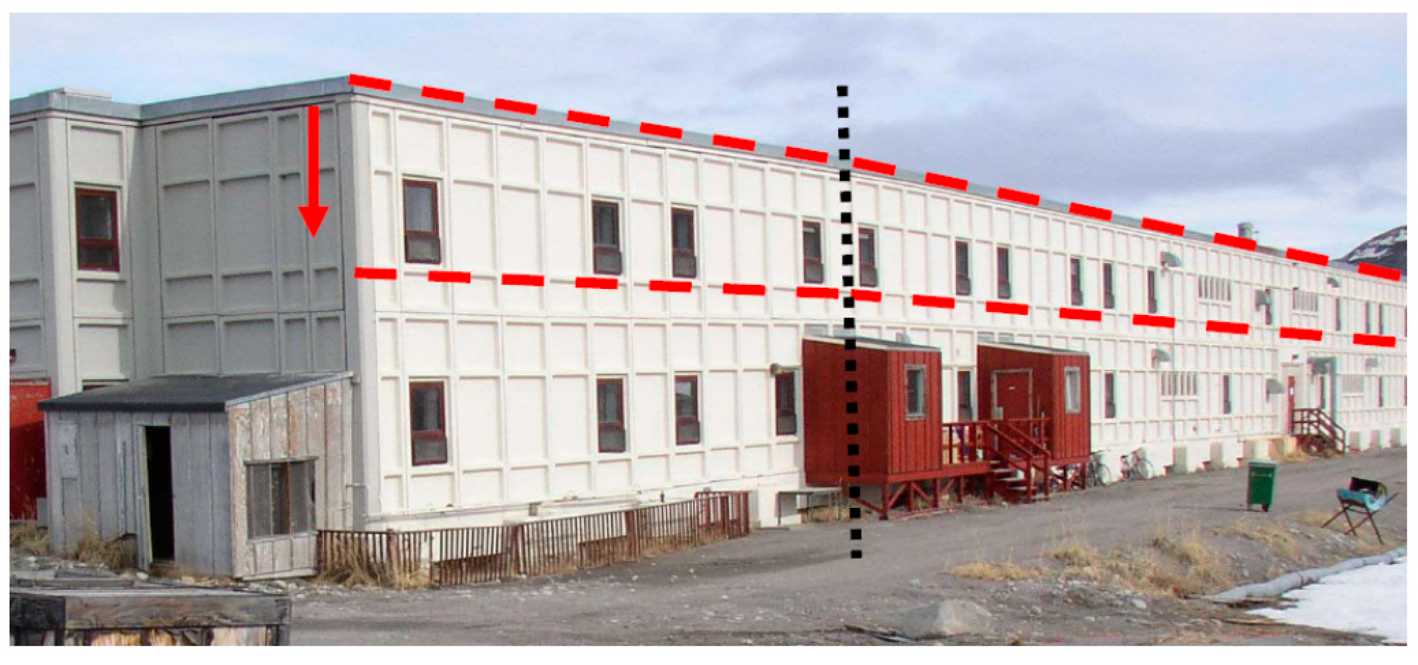
Hundreds of thousands of people in Alaska, Canada, Russia, and Greenland live on permafrost, a type of soil that covers nearly 24% of the northern hemisphere [1]. Frost heave and thawing actions are key issues in permafrost regions that can cause various engineering problems, such as the progressive lifting of sewer pipelines, subsidence of buildings, cracking of road surfaces, and damage to ground infrastructure structures or geological repository systems (Figure 1). Recently, we have seen that natural freeze-thaw cycles from season to season can also cause significant subsidence problems for buildings or underground structures, even in non-permafrost areas. The sequence of subsidence events caused by the frost heave and thawing cycle is depicted in Figure 2, which shows a homogeneous fine-grained soil column subjected to one-sided natural freezing from top-down. To analyze and predict this phenomenon, it is necessary to understand the complex thermal-hydro-mechanical (THM) coupling that occurs during the freezing process. The preconditions for frost heave action in frozen soil are as follows [2,3]: (a) the soil is potentially subject to frost heave action, (b) a sufficient supply of water, the material source for frost heave in soils, is available, and (c) the thermal conditions must be suitable to cause the freezing front to move at a sufficiently slow rate to allow for water migration.

In general, frozen soils comprise three zones: a frozen zone, a frozen fringe, and an unfrozen zone (Figure 3). The boundary between the frozen fringe and the unfrozen zone is called the freezing front, which is related to the 0 °C (273.15 K) isotherm [2]. When freezing begins in the frozen zone, the freezing front propagates to the unfrozen zone, resulting in an expansion in volume due to the phase change of the pore water behind the frozen fringe. Water subsequently moves into the freezing front to compensate for the water loss due to the phase change, forming a periodic ice layer referred to an ice lens [2,3,4,5]. The continuous growth of the ice lens ultimately causes a significant amount of frost heave.

Early research on the subject involved various experimental investigations aimed at understanding the frost heave action mechanism at various scales [6,7,8,9]. Such investigations covered small-scale column-freezing tests [6], large-scale tests [7], and long-term field-scale monitoring [8,9]. Afterwards, several numerical simulation studies based on heat and mass transfer in porous media were conducted to evaluate frost heave. Initially, such simulation models used empirical equations [10,11,12,13,14]. Konrad and Morgenstern [11] proposed the segregation potential (SP₀) theory, which explains the correlation between the temperature gradient (gradT) and the water flux in the frozen fringe according to the coefficient SP₀. Subsequently, Konrad and Duquennoi [14] proposed a thermodynamic model that treated soil as an incompressible material to derive new standards for ice lens formation. Shin et al. [15] developed an elasto-plastic mechanical constitutive equation for frozen soil using SP₀ to efficiently describe the complex THM phenomena of frozen soil. Zheng et al. [16] proposed a practical method that expands the one-dimensional frost heave equation (Takashi’s equation) into multi-dimensional situations.

Figure 1. Uneven permafrost thawing underneath a building foundation in Kangerlussuaq. (Re-printed with permission from ref. [17]. (photo by: Thomas Ingeman-Nielsen)).

Figure 1. Uneven permafrost thawing underneath a building foundation in Kangerlussuaq. (Re-printed with permission from ref. [17]. (photo by: Thomas Ingeman-Nielsen)).

Figure 2. The sequence of subsidence events caused by frost heave and thawing (Reproduced from [18]).

Figure 2. The sequence of subsidence events caused by frost heave and thawing (Reproduced from [18]).

Afterwards, a new approach was proposed to account for the fluid flow due to the temperature gradient. This approach estimated cryogenic suction using the interfacial tension between ice and fluid. Several studies used the Clausius–Clapeyron equation, which determines the ice-water pressure at phase equilibrium, to calculate cryogenic suction and perform THM analysis [19,20,21,22,23,24]. Aside from this, thermomechanical models have also been presented [2,25,26,27]. Although such models could not predict the formation of individual ice lenses, they effectively examined the global response of freezing soils by introducing a porosity rate function with no hydraulic analysis.

Meanwhile, due to the development of computer computational capabilities, prediction studies based on artificial neural networks are gaining traction. An ANN handles incomplete data and captures nonlinear and complex relationships among variables of a system. With these traits, ANNs have been recognized as a powerful tool for prediction. Similar to how ANNs are being applied in various engineering fields, the application of ANNs in the field of geotechnical engineering is also extending to various purposes, such as estimating ground surface settlement, in-situ permeability, undrained shear strength, thermal properties, and landslide susceptibility [28,29,30,31,32,33,34,35]. However, among many kinds of research, only a fraction of the studies was about predicting frost heave behavior [35]. Zhang et al. [35] predicted frost heave ratio of saline soil using back-propagation neural network (BPNN) and generalized regression neural network (GRNN) approaches and compared the prediction performance between two approaches to obtain a relatively reliable model.

Despite the significant progress brought upon by the aforementioned experimental, numerical, and statistical studies, several challenges remain. Most previous studies focused on the mathematical modeling of the freezing process accompanied by experimental validation, yet there remains a lack of in-depth analysis for freezing behavior from a geotechnical point of view. Most notably, the estimation of frost heave amount should be evaluated based on various geotechnical properties. Therefore, this study numerically evaluates the frost heave behavior of frozen soil at a specimen scale by considering important geotechnical parameters. A parametric study is also conducted to quantitatively analyze the effect of major geotechnical properties on frost heave behavior. In addition, after evaluating the sensitivity of each physical property to frost heave behavior via multiple statistical analyses, a prediction model based on an artificial neural network capable of practically estimating the frost heave ratio is finally presented.

Figure 3. Schematic representation of a frozen soil (Reproduced from [2]).

Figure 3. Schematic representation of a frozen soil (Reproduced from [2]).

2. Materials and Methods

This study conducted a THM analysis to evaluate the frost heave behavior of saturated specimens. The mathematical model constructed in this study was based on the constitutive equations introduced in previous studies [18,19,20,21,24]. Furthermore, the following assumptions were made to model the THM behavior of frozen soils:

• The soil is isotropic and elastic.
• The soil is a fully saturated medium that is fully frozen, partially frozen, or unfrozen.
• The water migration that occurs in the frozen fringe and the unfrozen zone follows Darcy’s law.
• The soil particles, pore water, and ice are incompressible under the pressure and temperature conditions present in cold regions, and these three-phase soil materials satisfy the local thermal equilibrium.

2.1. Mass Balance Equation

The volume fraction (θ) of a fully saturated soil can be expressed as the sum of the volumetric water content (θ_w) and the volumetric ice content (θ_i). It is also expressed as a function of the void ratio (e) and ice saturation (S_i). Ice saturation is a temperature-dependent function that can be estimated from an empirical function, such as that shown in Equation (2) [36].

$$\theta ={\theta }_w+{\theta }_i=\frac{e}{1+e}(1-S_i)+\frac{e}{1+e}{S}_i$$

(1)

$$S_i=\{\begin{array}{ll}1-{[1-(T-T_0)]}^{\alpha }& T\le T_0\\ 0& T\le T_0\end{array}$$

(2)

where T is the temperature (K), T₀ is the freezing temperature of pore water (T₀ = 273.15 K), and α is an empirical parameter.

The temperature gradient in a freezing soil causes the movement of pore water toward lower temperature regions under uniform pressure fields [37,38]. To simulate this phenomenon numerically, the mathematical formulation below is required. First, if a thermodynamic equilibrium is satisfied at the interface between the ice and pore water, the following relation is established between the temperature, ice pressure, and pore water pressure according to the Clapeyron equation, which is based on thermodynamics [39,40,41,42].

$$\frac{u_w}{{\rho }_w}-\frac{u_i}{{\rho }_i}=L\ln \frac{T}{T_0}$$

(3)

where ρ_w is the water density (kg/m³), ρ_i is the ice density (kg/m³), u_a is the atmospheric pressure (u_a = 101.3 kPa), and L is the latent heat of fusion (L = 334.5 kJ/kg).

The mass balance equation for the freezing behavior can be expressed as

$$\frac{\partial ({\rho }_w{\theta }_w)}{\partial t}dV+\frac{\partial ({\rho }_i{\theta }_i)}{\partial t}dV+{\rho }_w\nabla vdV=0$$

(4)

where t is the time and dV refers to the volume element of the soil. Assuming the pressure and temperature to be independent driving forces for the pore water flow, the velocity of the pore water v can be calculated as follows [43].

$$v=-k\nabla \psi =-k\nabla (z+\frac{u_w}{{\gamma }_w}+\frac{L}{g}\frac{\mathsf{\Delta }T}{T_0})$$

(5)

where ψ is the hydraulic head, which is defined as the sum of the elevation and pressure heads. k is the hydraulic conductivity (m/s), which is expressed as a function of temperature [12,13].

$$\frac{k}{k_0}=\{\begin{array}{ll}{[1-(T-T_0)]}^{\beta }& T\le T_0\\ 1& T>T_0\end{array}$$

(6)

where k₀ is the hydraulic conductivity in the unfrozen zone. β is an experimental parameter that varies with the size and structure of the pore, and its values are in the range of −8 to −40.

The volume element of the soil can be expressed with respect to the solid volume of the soil, and Equation (4) can be expanded as Equation (8).

$$dV=(1+e)d{V}_s$$

(7)

$$\frac{\partial }{\partial t}[{\rho }_{w}e(1-S_i)+{\rho }_{i}e{S}_i]+{\rho }_w(1+e)\nabla (-k\nabla \psi )=0$$

(8)

Rearrangement of these equations yields the final formula

$${\rho }_w(\frac{1}{1+e}\frac{\partial e}{\partial t}(1-S_i)-\frac{\partial S_i}{\partial t}\frac{e}{1+e})+{\rho }_i(\frac{1}{1+e}\frac{\partial e}{\partial t}{S}_i\frac{\partial S_i}{\partial t}\frac{e}{1+e})+{\rho }_w\nabla v=0$$

(9)

2.2. Energy Conservation Equation

The energy conservation equation for the freezing process is

$$\frac{\partial (\mathsf{\Phi }dV)}{\partial t}+\nabla QdV=0$$

(10)

where Φ is the heat content per unit volume, which contains the latent heat of fusion due to an increase in the ice content. C is the volumetric heat capacity of the frozen soil (J/m³/K), the subscript s, w, and i indicate the soil particle, pore water, and ice, respectively. Q refers to the heat flux per unit area (W/m²) and includes the effects of the heat conduction and convection of the pore water. λ_s, λ_w, and λ_i are the thermal conductivities (W/m·K) of the soil particles, pore water, and ice, respectively. The effective thermal conductivity λ is calculated by the geometric mean model.

$$\mathsf{\Phi }=CT-L\frac{e}{1+e}{S}_i{\rho }_i$$

(11)

$$C=\frac{e}{1+e}{C}_s{\rho }_s+\frac{e}{1+e}{C}_w{\rho }_w(1-S_i)+\frac{e}{1+e}{C}_i{\rho }_i{S}_i$$

(12)

$$Q=-\lambda \nabla T+C_w{\rho }_{w}vT$$

(13)

$$\lambda ={({\lambda }_s)}^{\frac{1}{1+e}}{({\lambda }_w)}^{\frac{e(1-S_i)}{1+e}}{({\lambda }_i)}^{\frac{e{S}_i}{1+e}}$$

(14)

Substituting Equations (7) and (11) into Equation (10) yields

$$\frac{\partial }{\partial t}(CT-L\frac{e}{1+e}{S}_i{\rho }_i)(1+e)d{V}_s+\nabla Q(1+e)d{V}_s=0$$

(15)

Rearrangement of these equations yields the final formula

$$(C-\frac{L{\rho }_{i}e}{1+e}\frac{\partial S_i}{\partial T})\frac{\partial T}{\partial t}-\frac{L{\rho }_i{S}_i}{1+e}\frac{\partial e}{\partial t}=\nabla {(\lambda \nabla T)}_s+C_{w}k\nabla \psi \nabla T$$

(16)

2.3. Force Equilibrium

The force equilibrium equation for the non-isothermal small deformation is

$$\nabla \sigma +\gamma =0$$

(17)

where σ is the total stress (Pa) and γ is the unit weight (Pa). Furthermore, the relationship between the total stress, effective stress, and the pore pressure is given by Equation (18); if the one-dimensional problem is considered, the stress-strain relationship for the compression specimen is given by Equation (19).

$$\sigma ={\sigma }^{\prime }+u_{por}$$

(18)

$$d{\sigma }^{\prime }=-E_{s}d{\epsilon }_v$$

(19)

Therefore, the force equilibrium equation can be expressed as

$$\nabla (-E_s\frac{e-e_0}{1+e_0})+\nabla u_{por}+\gamma =0$$

(20)

where e₀ refers to the initial void ratio.

2.4. Ice Lens Criteria

Many reports have proposed criteria concerning ice lens formation. For example, Everett [44] firstly proposed the frost theory, called a capillary theory. However, this theory had some limitations; the formation of discrete ice lenses was unclear, and the simulated results tended to underestimate the true values. Afterwards, the second frost theory was proposed. This theory considers zone with low water content, low hydraulic conductivity. In this theory, no frost heave exists between the freezing front and the frozen fringe. From this theoretical point of view, Konrad and Morgenstern [11] proposed a critical temperature at which the hydraulic conductivity locally decreases at the frozen fringe. Miller [45] and Gilpin [10] observed that ice lenses formed when the pore pressure was large enough to separate the soil particles. Additionally, based on the secondary theory, rigid ice was assumed. O’Neill [46] defined the criterion at which the pore pressure exceeds the total stress (i.e., the point at which the effective stress becomes zero) as the threshold for ice lens formation. Although there have been proposed various criteria concerning ice lens formation, this study used the ice lens formation threshold proposed by O’Neill [46] because the study also assumes that the ice segregation may occur behind the frozen fringe at which the effective stress becomes zero.

3. Evaluation of Frost Heave Ratio

Using the governing equations described above, we performed a THM analysis to predict frost heave for a saturated soil specimen. The material properties used in the numerical model are presented in

Table 1. Material properties used in FE model.

Parameter	Value	Unit
Density of porewater, ρw	1000	kg/m3
Density of ice ρi	917	kg/m3
Density of solid particle, ρs	2600	kg/m3
Heat capacity of water at constant pressure, Cw	4180	J/kg/K
Heat capacity of ice at constant pressure, Ci	2044	J/kg/K
Heat capacity of solid particle at constant pressure, Cs	831	J/kg/K
Latent heat of fusion, L	334.5	kJ/kg
Thermal conductivity of water, λw	0.56	W/m/K
Thermal conductivity of ice, λi	2.24	W/m/K
Melting point, T0	0	°C
Young’s modulus, Es	1.2	MPa

. The governing equations are highly non-linear, and thus, the commercial finite element (FE) software COMSOL Multiphysics [47] was used to solve the complex differential equations. Furthermore, the numerical simulation was implemented for a one-dimensional freezing test. The depth of the soil specimen was set as 100 mm, and the initial temperature of the entire specimen was set as 5 °C. The analysis was conducted until thermal equilibrium was achieved while maintaining constant bottom and top boundary temperatures (Top boundary temperature was set as 5 °C and bottom boundary temperature was set as −5 °C and hence the temperature gradient was 1 °C/cm). The groundwater level (GWL) was fixed at the bottom boundary to allow for a continuous water supply during freezing, and the overburden pressure applied on the top boundary was set to atmospheric pressure (101.3 kPa). The frost heave ratio was obtained using Equation (21).

$$\varsigma (\%)=\frac{\mathsf{\Delta }{H}_f}{H_0}$$

(21)

where ζ is the frost heave ratio (%). ΔH_f is the amount of total heave (mm), H₀ is initial specimen height (mm), and Δt is the elapsed time (h).

Figure 4 shows the variation of frost heave ratio (ζ) and the position of the freezing front over time obtained from the simulation model. The propagation rate of the freezing front gradually slowed down as time passed: the freezing front propagated rapidly during the initial stages of freezing but came to a halt as it approached thermal equilibrium. The amount of frost heave also steadily increased until thermal equilibrium was achieved. After reaching thermal equilibrium (approximately after 60 h), the freezing front no longer moved, and no further severe frost heave occurred. Overall, the amount of frost heave increased in a nonlinear manner with time, a tendency that was also observed in the experimental results of Konrad and Morgenstern [11]. In Figure 4, the calculated frost heave ratio at 60 h was approximately 8%.

To verify the reliability of these simulation results, we compared the results with those of the previous numerical studies for the same freezing conditions. As shown in Figure 5, the predictions of the model for the pore pressure and temperature with specimen depth showed good agreement with the results of Zhou and Li [21]. This suggests that the numerical model used in this study is reliable.

A parametric study was subsequently conducted to quantitatively analyze the effects of geotechnical properties on the frost heave ratio. This study considered the thermal conductivity and initial hydraulic conductivity of the soil particles as crucial parameters. This is because frost heave behavior is mainly determined by the propagation rate of the freezing front and the water supply in the frozen zone. Whereas the particle thermal conductivity affects the propagation rate of the freezing front, the initial hydraulic conductivity is concerned with the inflow of pore water in the unfrozen zone. Thus, we used the numerical simulation model to obtain and mutually compare frost heave ratio values according to a total of 251 influencing parameter combinations. As shown in Figure 6, the amount of heave tends to decrease as the particle thermal conductivity increases. This is because the freezing rate becomes too high if freezing is accelerated due to the high thermal conductivity of the particles, resulting in thermal conditions that prevent a sufficient inflow of water from external sources. On the other hand, the frost heave ratio has a positive correlation with initial hydraulic conductivity: as the initial hydraulic conductivity increases, the frost heave ratio tends to increase. In other words, if the thermal conditions are kept the same and the hydraulic conditions are altered, a higher soil hydraulic conductivity would result in a higher frost heave ratio. However, it should be noted that these phenomena are only valid for silty soil, which is potentially subject to frost heave action. If the soil specimen is closer to sandy soil, no capillary action occurs, resulting in insignificant amounts of heave, regardless of the permeability.

Meanwhile, in order to investigate the sensitivity of both the thermal and hydraulic conductivities of frozen soils on the frost heave ratio, a correlation analysis and regression analysis were conducted.

Table 2. Pearson correlation analysis between the three variables.

		λs	k0	ζ
λs	Correlation coefficient	1	0.114	−0.330 **
	p-value (two sided)		>0.1	0.000
k0	Correlation coefficient	0.114	1	0.805 **
	p-value (two sided)	>0.1		0.000
ζ	Correlation coefficient	−0.330 **	0.805 **	1
	p-value (two sided)	0.000	0.000

* Correlation coefficient is significant at two sides (p < 0.05). ** Correlation coefficient is significant at two sides (p < 0.01).

shows the results of the Pearson correlation analysis for each variable [48]. The analysis illustrates that both the thermal conductivity and initial hydraulic conductivity of a frozen soil can significantly affect the heave ratio, as the p-value of each parameter was less than 0.05 (Table 2). Furthermore, this study also conducted a regression analysis, as shown in

Table 3. Regression analysis between three variables.

	B	Standard Error	t	p-Value	VIF
Constant	6.958	0.104	66.655
Hydraulic conductivity	7.68 × 109	2.41 × 108	31.963	<0.01	1.013
Thermal conductivity	−0.372	0.023	−16.011	<0.01	1.013
R2	0.829
adjR2	0.827

B: non-standardized coefficient, t: B/standard error, VIF: variance inflation.

. According to the regression analysis, the p-values of the coefficients for thermal conductivity and initial hydraulic conductivity were also lower than 0.05, which indicates that these two variables can significantly affect the heave ratio [49]. Although a significant correlation was confirmed between the independent and dependent variables, it was confirmed that an auto-correlation exists in the dependent variable. Therefore, in this study, it was judged that it would be more beneficial to propose a predictive model for frost behavior using an artificial neural network instead of deriving a regression equation.

4. Prediction of Frost Heave Ratio Using the Artificial Neural Network Model

4.1. Establishment of an Artificial Neural Network

In this study, an ANN for the estimation of frost heave ratio was designed with three layers: an input layer, a hidden layer, and an output layer. The input layer stores and provides data to the ANN network, whereas the hidden layer, which is constructed with general neurons, connects the input layer to the output layer. As shown in Figure 7, the developed ANN model has a 2-5-1 structure: with two neurons in the input layer, five neurons in the hidden layer, and one neuron in the output layer. Each neuron has an input parameter that is the weighted sum of the output from every neuron in the previous layer. This sum is passed through a transfer function to provide an outgoing signal to the next layer. Finally, the output layer stores the value predicted by the network. For each neuron, the total input value can be obtained as follows.

$$z=Wx+b$$

(22)

where W is the weight matrix, which stores the weights of every connection between the current and the preceding layer. A vector x contains all output signal values from the previous layer, whereas the vector b comprises the bias value at the current layer. The input value is transformed within neurons via a transfer function. Thus, Equation (22) can rewrite as follows.

$$y=f\left(Wx+b\right)$$

(23)

where f is the transfer function, which usually adds non-linearity to the network to try to fit the network. Therefore, the network is able to produce an output that fits within the proper value. Without transfer functions, the network could only be able to provide a linear output when compared with its input signal.

To guarantee the performance of the network, the Nguyen-Widrow method [50] was adopted to produce the initial weight and bias. In this study, the back-propagation technique was applied to the training procedure. According to this method, the procedure includes two phases. First, the feed-forward phase involves the passing of all data from the input layer to the output layer according to the weighted sum of the output from every connected neuron in the preceding layer. A transfer function is applied to estimate the output value within neurons. Thus, the predicted output is estimated at the output layer. The difference between the predicted value and the expected value is obtained by a cost function. In this study, the quadratic cost function was applied as follows.

$$C={\displaystyle \sum {\left(y_i-{\exp }_i\right)}^2}$$

(24)

where y_i is the predicted value obtained by ANN while exp_i is the expected value from the dataset. In Equation (24), the predicted value is obtained by variables that contain input signal, weight, biases, transfer function, and the expected value. Therefore, the cost function can be rewritten as follows.

$$C\left(W,b,f\left(y\right),y,x,\exp \right)$$

(25)

Secondly, the backward pass computes the loss function and updates the weight matrix. This process is repeated until the sum squared error over all epochs is minimized. With every training iteration, a new weight W⁺ can be obtained based on the cost function and current weight W.

$$W^{+}=W-\eta \nabla C$$

(26)

where η is learning rate, which is usually a small constant. ∇C is the gradient of the cost function with respect to the weight and can be estimated as follows.

$$\nabla C={\left[\begin{array}{cccc}\partial C/\partial w_1& \partial C/\partial w_2& \cdots & \partial C/\partial w_n\end{array}\right]}^T$$

(27)

One of the most frequently encountered problems is overfitting, which occurs during training procedures. Overfitting occurs when ANN model is overly trained with training data and fails to evaluate the testing data. In this study, we have investigated the effect of Bayesian regularization and Levenberg Marquardt.

The Bayesian regularization technique can be applied to guarantee the efficiency of the ANN training process. This study also applied the Bayesian regularization technique. The training process reduces the sum of squared errors, which can be denoted F = F_D. However, the Bayesian regularization adds some terms to construct the objective function as follows.

$$F=\beta E_D+\alpha E_W$$

(28)

where E_D is the sum of squared errors, E_w is the sum of the square of the weight matrix of the ANN model. α and β are the objective function parameters. Both objective function parameters can be obtained via the Gauss-Newton Approximation method.

The Levenberg Marquardt technique is used to solve the non-linear least squares problem that is combined the Gaussian-Newton method and the Steepest Decent method. The new weights are calculated using the following equation

$$W_{t+1}=W_t-{\left({\mathbf{J}}^T\mathbf{J}+\mu \mathbf{I}\right)}^{-1}{\mathbf{J}}^T{\mathbf{E}}_i$$

(29)

where I is identity unit matrix, μ is a learning parameter. J is the Jacobian matrix and E is cumulative error vector which is determined as following [51]. For the learning rate of μ = 0, the Gauss-Newton method is adapted while the Steepest Decent is applied within larger learning rate. The learning rate μ is automatically adjusted at each iteration. The disadvantage of Lenvenberg Marquardt requires the high computational cost to compute the large Jacobians and inverting matrixes.

4.2. Application of an ANN to Frost Heave Ratio Predictions

In this study, an ANN model was developed to predict the frost heave ratio ζ for the frozen soil. In the ANN model, two parameters-hydraulic conductivity in the unfrozen zone (k₀) and the thermal conductivity of the soil particle (λ_s)-were considered as input parameters. The training data included input-target pairs: 197 pairs for training and 49 pairs for testing. Bayesian regularization was applied to a back-propagation neural network.

The architecture of an ANN is usually determined via trial and error. Generally, the input-target pairs scale in the range of [−1, 1] before training. Thus, the minimum and maximum values of the original input-target pairs are scaled to “−1” and “1”, respectively. After the training procedure, the weights matrix and bias vectors are applied to any future inputs, which should be scaled based on the minimum-maximum pairs of the original inputs and targets. Once the network is trained, the predicted value falls within the range [−1, 1]. The predicted value should be converted back into the same units by vector contains the minimum and maximum of the original input-targets pair. In this study, the tangent sigmoid transfer function $f\left(x\right)=2/{\left(1+e^{-2x}\right)}^{-1}$ is adopted for all layers except for the input layer where the linear transfer function $f\left(x\right)=x$ is used instead.

Additionally, the learning rate (in Equation (28)) plays a vital role in the ANN network. If the learning rate is too low, the weight matrix updates at an inadequate rate and the local minimum may take a long time to achieve. In contrast, an overly large learning rate may result in the network overreaching and missing the local minimum optima. Traditionally, many studies adopted learning rate of 0.1 or 0.01. In our study, we investigated the effect of both learning rates on the ANN model.

Figure 8 shows the relationship between the coefficient of determination R² and the number of neurons in the hidden layer for Bayesian Regularization and Levenberg Marquardt according to both learning rates (η = 0.01 and η = 0.1). The R² converged to a high value (R² ≥ 0.95) when the ANN model had more than three neurons and six neurons in the hidden layer for Bayesian Regularization and Levenberg Marquardt, respectively. Although the Levenberg Marquardt algorithm achieved a higher converged coefficient compared to those of Bayesian Regularization at eight and ten neurons in the hidden layer but it requires a high computational cost for computing Jacobian matrix. Thus, the Bayesian Regularization was adopted in this study. With a learning rate of 0.01, the R² value of the ANN model based on the Bayesian Regularization peaked highest at five neurons in the hidden layer. Therefore, the learning rate and the number of neurons in the hidden layer were set as 0.01 and 5, respectively. Figure 9 shows the relationship between the converged coefficient R² and the number of neurons in the hidden layer of the ANN model based on the Bayesian Regularization according to the performance functions that consist of Mean Absolute Error (MAE), Mean Square Error (MSE), Sum Absolute Error (SSA), and Sum Square Error (SSE). The convergence coefficient peaked at five neurons in the hidden layer when the performance function was mean square error (MSE). Other performance functions were similar trending but they had a lower value of converged coefficient R². In this study, the Mean Square Error (MSE) was adopted to evaluate the performance of the ANN model.

Figure 10 illustrates a comparison of the frost heave ratio predicted by the ANN model and simulation model. The model exhibited R² value of 0.9538 for training data and 0.8929 for the testing data. Thus, it can be judged that the proposed ANN-based prediction model is reliable and applicable for predicting the frost heave ratio using hydraulic conductivity in the unfrozen zone and the thermal conductivity of the soil particle. However, it should be noted that that the inherited error can be involved in ANN and probably multiplied by the estimation error when ANN is implemented because FEM itself contains inherited modeling error.

Table 4. Weighs and biases of the trained ANN model.

	First Layer					Second Layer
Weight	−1.3290	1.1272	−0.8410	−0.9127	0.7730	−0.5700
	1.5107	−0.2495	−0.0200	0.6520	1.1022	−1.1663
						−0.4456
						1.2482
						0.5838
Bias	−0.1840					−0.4895
	−1.8576
	−1.0096
	−0.5137
	−0.5254

and Figure 11 present the weights and biases for the trained model, which ultimately allows others to make practical use of the developed ANN model.

In order to determine the sensitivity of the ANN model, the Garson analysis [52] was adopted to calculate the interpreting of the connection weights that indicate the importance of the input weights importance. The interpreting of the connection weights along the connection from the input to output can be calculated as follows.

$$\frac{{\displaystyle {\sum }_j^{N_H}\left(\frac{I_{V_j}}{{\displaystyle {\sum }_k^{N_V}{I}_{V_j}}}{O}_j\right)}}{{\displaystyle {\sum }_i^{N_V}{\displaystyle {\sum }_j^{N_H}\left(\frac{I_{V_j}}{{\displaystyle {\sum }_k^{N_V}{I}_{V_j}}}{O}_j\right)}}}$$

(30)

where N_H and N_V are the number of the neurons in the hidden layers and the number of the variable (input parameters). I_V is the sum the product of the input connection weight in the hidden layer while O is the connection weight of the output node.

Table 5. The neural−network connection for the ANN model.

Input Layer Connections
k0 (m/s) FROM:	−1.3290	1.1272	−0.8410	−0.9127	0.7730
λs (W/m.K) FROM:	1.5107	−0.2495	−0.0200	0.6520	1.1022
Hidden layer connections
Hidden node #1
BIAS:		−0.1840
TO:		−1.3290	1.5107
FROM:		−0.5700
Hidden node #2
BIAS:		−1.8576
TO:		1.1272	−0.2495
FROM:		−1.1663
Hidden node #3
BIAS:		−1.0096
TO:		−0.8410	−0.0200
FROM:		−0.4456
Hidden node #4
BIAS:		−0.5137
TO:		−0.9127	0.6520
FROM:		1.2482
Hidden node #5
BIAS:		−0.5254
TO:		0.7730	1.1022
FROM:		0.5838
Output layer connections
Heavy ratio ζ (%)
BIAS:	−0.4895
TO:	−0.5700	−1.1663	−0.4456	1.2482	0.5838

illustrates the connection weights and bias for each layer.

Table 6. The interpreting neural−network connection weights.

Hidden Node
	V1	V2	OUT
Connection weights (Input to hidden)
1	−1.3290	1.5107	−0.5700
2	1.1272	−0.2495	−1.1663
3	−0.8410	−0.0200	−0.4456
4	−0.9127	0.6520	1.2482
5	0.7730	1.1022	0.5838
Absolute connection weights (input to hidden)
1	1.3290	1.5107	0.5700
2	1.1272	0.2495	1.1663
3	0.8410	0.0200	0.4456
4	0.9127	0.6520	1.2482
5	0.7730	1.1022	0.5838
Connection shares * hidden node input
1	0.2668	0.3032
2	0.9549	0.2114
3	0.4352	0.0104
4	0.7281	0.5201
5	0.2407	0.3431
Sum:	2.6257	1.3882
Input node share of output layer connections, excluding bias ones
	65.41%			34.59%
	k0 (m/s)			λs (W/M·K)

demonstrated that the hydraulic conductivity in the unfrozen zone (k₀) was the most important input factor while the thermal conductivity of the soil particle (λ_s) was lesser importance.

5. Summary and Conclusions

The present study evaluated the frost heave amount caused by the formation of an ice lens layer during the freezing process of soils. Through a parametric study, we analyzed the effects of geotechnical parameters on frost heave ratio in a quantitative manner. Furthermore, this study proposed a predictive model based on an artificial neural network capable of practically estimating frost heave ratio. The main conclusions drawn from this study are as follows.

• A fully coupled THM model numerically evaluated various physical phenomena that occur during one−dimensional freezing. During the freezing process, the freezing front propagated rapidly when freezing initially began but came to a halt as it approached thermal equilibrium. The amount of frost heave increased steadily until thermal equilibrium was achieved, after which the freezing front stopped and no further severe frost heave occurred.
• According to the results of the parametric study, the overall patterns of the predictive model are explained by preconditions for frost heave action. The amount of heave tended to decrease as particle thermal conductivity increased. This may have something to do with thermal conditions that prevent a sufficient inflow of water from external sources due to a high freezing rate. Additionally, the frost heave ratio tended to increase as the initial hydraulic conductivity increased. If the thermal conditions are the same yet the hydraulic conditions are varied, it could be judged that higher soil hydraulic conductivity would result in a higher frost heave ratio.
• After evaluating the sensitivity of each parameter to frost heave behavior through multiple statistical analyses, an artificial neural network model was proposed to practically estimate frost heave behavior. According to the interpreting connection weights, the hydraulic conductivity in the unfrozen zone (k₀) was the most important input parameter that was a direct cause of the frost heave ratio ζ(%), and the thermal conductivity of the soil particle (λ_s) was lesser importance. In order to evaluate the applicability of the artificial neural network model, the model was tested with datasets that had not been introduced during the training stage. According to the verification results, the trained network model demonstrated a reliable accuracy (R² = 0.893) in predicting frost heave ratio, even when the model used the test datasets that were not part of the training datasets. It is expected that this prediction model will be useful in many areas of research related to evaluating the frost heave behavior of saturated specimens.

References

1. National Snow and Ice Data Center. All about Frozen Ground. Available online: https://nsidc.org/cryosphere/frozenground/index.html (accessed on 18 January 2018).
2. Michalowski, R.L.; Zhu, M. Frost heave modelling using porosity rate function. Int. J. Numer. Anal. Meth. Geomech. 2006, 30, 703–722. [Google Scholar] [CrossRef] [Green Version]
3. Zhang, Y. Thermal-Hydro-Mechanical Model for Freezing and Thawing of Soils. Ph.D. Thesis, Civil Engineering at University of Michigan, Ann Arbor, MI, USA, 2014. [Google Scholar]
4. Konrad, J.M. Frost susceptibility related to soil index properties. Can. Geotech. J. 1999, 36, 403–417. [Google Scholar] [CrossRef]
5. Wu, D.; Lai, Y.; Zhang, M. Heat and mass transfer effects of ice growth mechanisms in a fully saturated soil. Int. J. Heat Mass Transf. 2015, 86, 699–709. [Google Scholar] [CrossRef]
6. Penner, E. Aspects of ice lens growth in soils. Cold Reg.Sci. Technol. 1986, 13, 91–100. [Google Scholar] [CrossRef] [Green Version]
7. Harris, C.; Smith, J.S.; Davies, M.C.R.; Rea, B. An investigation of periglacial slope stability in relation to soil properties based on physical modelling in the geotechnical centrifuge. Geomorphology 2008, 93, 437–459. [Google Scholar] [CrossRef]
8. Harris, C. Physical modelling of periglacial solifluction: Review and future strategy. Permafrost Periglac. Process. 1996, 7, 349–360. [Google Scholar] [CrossRef]
9. Harris, C.; Luetschg, M.; Davies, M.C.R.; Smith, F.; Christiansen, H.H.; Isaksen, K. Field instrumentation for real-time monitoring of periglacial solifluction. Permafr. Periglac. Process. 2007, 18, 105–114. [Google Scholar] [CrossRef]
10. Gilpin, R.R. A model for the prediction of ice lensing and frost heave in soils. Water Resour. Res. 1980, 16, 918–930. [Google Scholar] [CrossRef]
11. Konrad, J.M.; Morgenstern, N.R. A mechanistic theory of ice lens formation in fine-grained foils. Can. Geotech. J. 1980, 17, 473–486. [Google Scholar] [CrossRef]
12. O’Neill, K.; Miller, R.D. Exploration of a rigid ice model of frost heave. Water Resour. Res. 1985, 21, 281–296. [Google Scholar] [CrossRef]
13. Nixon, J.F.D. Discrete ice lens theory for frost heave in soils. Can. Geotech. J. 1991, 28, 843–859. [Google Scholar] [CrossRef]
14. Konrad, J.M.; Duquennoi, C. A model for water transport and ice lensing in freezing soils. Water Resour. Res. 1993, 29, 3109–3124. [Google Scholar] [CrossRef]
15. Shin, H.S.; Kim, J.M.; Lee, J.; Lee, S.R. Mechanical Constitutive Model for Frozen Soil. J. Korean Geotech. Soc. 2012, 28, 85–94. [Google Scholar] [CrossRef] [Green Version]
16. Zheng, H.; Kanie, S.; Niu, F.; Akagawa, S.; Li, A. Application of practical one-dimensional frost heave estimation method in two-dimensional situation. Soils Found. 2016, 56, 904–914. [Google Scholar] [CrossRef]
17. Ingeman-Nielsen, T. Lecture Notes—11854 Infrastructure Construction in the Arctic; ARTEK and DTU Byg: Kongens Lyngby, Denmark, 2017. [Google Scholar]
18. Cicchetti, L. Thermo-Hydro-Mechanical Simulations of Artificial Ground Freezing. Master’s Thesis, Cold Climate Engineering, Departments of Civil and Environmental Engineering at NTNU and DTU, Trondheim, Norway, 2018. [Google Scholar]
19. Thomas, H.R.; Cleall, P.; Li, Y.C.; Harris, C.; Kern-Luetschg, M. Modeling of cryogenic processes in permafrost and seasonally frozen soils. Geotechnique 2009, 59, 173–184. [Google Scholar] [CrossRef]
20. Liu, Z.; Yu, X. Coupled thermo-hydro-mechanical model for porous materials under frost action: Theory and implementation. Acta Geotechnica 2011, 6, 51–65. [Google Scholar] [CrossRef]
21. Zhou, J.; Li, D. Numerical analysis of coupled water, heat and stress in saturated freezing soil. Cold Reg. Sci. Technol. 2012, 72, 43–49. [Google Scholar] [CrossRef]
22. Zhou, M.M. Computational Simulation of Soil Freezing: Multiphase Modeling and Strength Upscaling. Ph.D. Dissertation, Ruhr University Bochum, Bochum, Germany, 2013. [Google Scholar]
23. Zhou, M.M.; Meschke, G. A three-phase thermo-hydro-mechanical finite element model for freezing soils. Int. J. Numer. Anal. Meth. Geomech. 2013, 37, 3173–3193. [Google Scholar] [CrossRef]
24. Lai, Y.; Pei, W.; Zhang, M.; Zhou, J. Study on theory model of hydro-thermal–mechanical interaction process in saturated freezing silty soil. Int. J. Heat Mass Transfer. 2014, 78, 805–819. [Google Scholar] [CrossRef]
25. Michalowski, R.L. A constitutive model of saturated soils for frost heave simulations. Cold Reg. Sci. Technol. 1993, 22, 47–63. [Google Scholar] [CrossRef]
26. Zhang, Y.; Michalowski, R.L. Thermal-Hydro-Mechanical Analysis of Frost Heave and Thaw Settlement. J. Geotech. Geoenviron. Eng. 2015, 141, 04015027. [Google Scholar] [CrossRef]
27. Liu, H.; Maghoul, P.; Shalaby, A.; Bahari, A. Thermo-Hydro-Mechanical Modeling of Frost Heave Using the Theory of Poroelasticity for Frost-Susceptible Soils in Double-Barrel Culvert Sites. Trans Geotech. 2019, 20, 100251. [Google Scholar] [CrossRef]
28. Lee, Y.G.; Yoon, Y.W.; Kang, B.H. Prediction of undrained shear strength of normally consolidated clay with varying consolidation pressure ratios using artificial neural networks. J. KGS 2000, 16, 75–81. [Google Scholar]
29. Min, T.K.; Hwang, K.M.; Jeon, H.W. Prediction of consolidation settlements at vertical drain using modular artificial neural networks. J. KGS 2000, 16, 71–77. [Google Scholar]
30. Kim, Y.S. Development of neural network nodel for estimation of undrained shear strength of Korean soft soil based on UU triaxial test and piezocone test results. J. KGS 2005, 21, 73–84. [Google Scholar]
31. Go, G.H.; Lee, S.R.; Kim, Y.S. A reliable model to predict thermal conductivity of unsaturated weathered granite soils. Int. Commun. Heat Mass Transf. 2016, 74, 82–90. [Google Scholar] [CrossRef]
32. Yoon, S.; Jeon, J.S.; Kim, G.Y.; Seong, J.H.; Baik, M.H. Specific heat capacity model for compacted bentonite buffer materials. Ann. Nucl. Energy 2019, 125, 18–25. [Google Scholar] [CrossRef]
33. Bragagnolo, L.; da Silva, R.V.; Grzybow, J.M.V. Artificial neural network ensembles applied to the mapping of landslide susceptibility. Catena 2020, 184, 104240. [Google Scholar] [CrossRef]
34. Kim, C.Y.; Bae, G.J.; Hong, S.W.; Park, C.H.; Moon, H.K.; Shin, H.S. Neural network based prediction of ground surface settlements due to tunnelling. Compu. Geot. 2001, 28, 517–547. [Google Scholar] [CrossRef]
35. Zhang, X.; Wang, Q.; Huo, Z.; Yu, T.; Wang, G.; Liu, T.; Wang, W. Prediction of Frost-Heaving Behavior of Saline Soil in Western Jilin Province, China, by Neural Network Methods. Math. Probl. Eng. 2017, 6, 1–10. [Google Scholar] [CrossRef] [Green Version]
36. Tice, A.R.; Anderson, D.M.; Banin, A. The Prediction of Unfrozen Water Contents in Frozen Soils from Liquid Limit Determinations; Cold Regions Research & Engineering Laboratory, U.S. Army Corps of Engineers: Washington, DC, USA, 1976. [Google Scholar]
37. Hoekstra, P. Moisture movement in soils under temperature gradients with the cold-side temperature below freezing. Water Resour. Res. 1966, 2, 241–250. [Google Scholar] [CrossRef]
38. Mageau, D.W.; Morgenstern, N.R. Observations on moisture migration in frozen soils. Can. Geotech. J. 1980, 17, 54–60. [Google Scholar] [CrossRef]
39. Kay, B.D.; Groenevelt, P.H. On the interaction of water and heat transport in frozen and unfrozen soils: I. Basic theory; The vapor phase. Soil Sci. Soc. Am. J. 1974, 38, 395–400. [Google Scholar] [CrossRef]
40. Black, P.B. Applications of the Clapeyron Equation to Water and Ice in Porous Media; Cold Regions Research & Engineering Laboratory, U.S. Army Corps of Engineers: Washington, DC, USA, 1995. [Google Scholar]
41. Henry, K.S. A review of the thermodynamics of frost heave. CRREL US Army Corps Eng. 2000, 1–26. [Google Scholar]
42. Chen, F.X.; Song, Z.P.; Li, N. Study on moisture migrating force model of freezing soil base on adsorption-film moisture migration mechanism. J. Water Resour. Arch. Eng. 2006, 4, 1–4, (In Chinese with English Abstract). [Google Scholar]
43. Nakano, Y. Quasi-steady problems in freezing soils. 1. Analysis on the steady growth of an ice layer. Cold Reg. Sci. Technol. 1990, 17, 207–226. [Google Scholar] [CrossRef]
44. Everett, D.H. The thermodynamics of frost damage to porous solids. Trans. Faraday Soc. 1961, 57, 1541–1551. [Google Scholar] [CrossRef]
45. Miller, R.D. Freezing and heaving of saturated and unsaturated soils. Highw. Res. Rec. 1972, 393, 1–11. [Google Scholar]
46. O’Neill, K. The physics of mathematical frost heave models: A review. Cold Reg. Sci. Technol. 1983, 6, 275–291. [Google Scholar] [CrossRef]
47. COMSOL Inc. Introduction to Comsol Multiphysics; COMSOL Inc.: Burlington, VT, USA, 2021. [Google Scholar]
48. Cohen, J. Statistical Power Analysis for the Behavioral Sciences, 2nd ed.; Lawrence Erlbaum Associates: Hillsdale, NJ, USA, 1988. [Google Scholar]
49. Lee, I.H. Easy Flow Regression Analysis; Hannarae Publishing Corporation: Seoul, Korea, 2014. [Google Scholar]
50. Nguyen, D.; Widrow, B. Improving the learning speed of 2-layer neural networks by choosing initial values of the adaptive weights. In Proceedings of the International Joint Conference on Neural Networks, San Diego, CA, USA, 17–21 June 1990; Volume 3, pp. 21–26. [Google Scholar]
51. Wilamowski, B.M.; Chen, Y.; Malinowski, A. Efficient algorithm for training neural networks with one hidden layer. In Proceedings of the IJCNN’99. International Joint Conference on Neural Networks, Washington, DC, USA, 10–16 July 1999; Volume 3, pp. 1725–1728. [Google Scholar] [CrossRef] [Green Version]
52. Garson, G.D. Interpreting Neural Network Connection Weights. AI Expert. 1991, 6, 47–51. [Google Scholar] [CrossRef]
Figure 4. Frost heave ratio and frost front position with time.
Applsci 11 10834 g004
Figure 5. Comparison results with those of the previous numerical studies [21] for the 1D freezing.
Applsci 11 10834 g005
Figure 6. Effect of geotechnical properties on the frost heave ratio.
Applsci 11 10834 g006
Figure 7. Artificial neural network model for estimating the frost heave ratio.
Applsci 11 10834 g007
Figure 8. Relationship between R2 value and number of neurons in the hidden layer according to learning rate for Bayesian Regularization and Levenberg Marquardt.
Applsci 11 10834 g008
Figure 9. Relationship between R2 value and number of neurons in the hidden layer according to the performance functions within Bayesian Regularization.
Applsci 11 10834 g009
Figure 10. Comparison of the frost heave ratio and its predicted value as obtained by the ANN.
Applsci 11 10834 g010
Figure 11. Weights and Biases of the ANN network.
Applsci 11 10834 g011