Next Article in Journal
Response of Mechanical Properties of Polyvinyl Chloride Geomembrane to Ambient Temperature in Axial Tension
Next Article in Special Issue
Edge and Notch Detection in a Plate Using Time Reversal Process of Leaky Lamb Waves
Previous Article in Journal
Analytical Model to Calculate Radial Forces in Permanent-Magnet Synchronous Machines
Previous Article in Special Issue
Numerical Simulation of Enhanced Photoacoustic Generation and Wavefront Shaping by a Distributed Laser Array
 
 
Correction published on 20 January 2022, see Appl. Sci. 2022, 12(3), 1043.
Article

Towards Explainable Augmented Intelligence (AI) for Crack Characterization

by
Larissa Fradkin
1,*,
Sevda Uskuplu Altinbasak
1,† and
Michel Darmon
2
1
Sound Mathematics Ltd., 11 Mulberry Close, Cambridge CB4 2AS, UK
2
Université Paris-Saclay, CEA, List, F-91120 Palaiseau, France
*
Author to whom correspondence should be addressed.
Current Address: ARM, 110 Fulbourn Road, Cambridge CB1 9NJ, UK.
Appl. Sci. 2021, 11(22), 10867; https://doi.org/10.3390/app112210867
Submission received: 23 October 2021 / Revised: 12 November 2021 / Accepted: 12 November 2021 / Published: 17 November 2021 / Corrected: 20 January 2022
(This article belongs to the Special Issue Ultrasonic Modelling for Non-destructive Testing)

Abstract

:
Crack characterization is one of the central tasks of NDT&E (the Non-destructive Testing and Evaluation) of industrial components and structures. These days data necessary for carrying out this task are often collected using ultrasonic phased arrays. Many ultrasonic phased array inspections are automated but interpretation of the data they produce is not. This paper offers an approach to designing an explainable AI (Augmented Intelligence) to meet this challenge. It describes a C code called AutoNDE, which comprises a signal-processing module based on a modified total focusing method that creates a sequence of two-dimensional images of an evaluated specimen; an image-processing module, which filters and enhances these images; and an explainable AI module—a decision tree, which selects images of possible cracks, groups those of them that appear to represent the same crack and produces for each group a possible inspection report for perusal by a human inspector. AutoNDE has been trained on 16 datasets collected in a laboratory by imaging steel specimens with large smooth planar notches, both embedded and surface-breaking. It has been tested on two other similar datasets. The paper presents results of this training and testing and describes in detail an approach to dealing with the main source of error in ultrasonic data—undulations in the specimens’ surfaces.

1. Introduction

The aim of this paper is to address a challenge of developing an explainable AI for semi-automatic crack characterization, with a view to its ultimate deployment in ultrasonic units for NDT&E (the Non-destructive Testing and Evaluation) of industrial components and structures. Since the most advanced units are phased arrays of ultrasonic transducers all the experimental data used to train and test the AI discussed below have been collected using linear arrays of this nature. Moreover, the experiments have been designed to emulate cracks and inspection surfaces typically encountered in walls of nuclear reactors. It is particularly important to minimize human involvement in interpretation of NDT data in nuclear industry: With the new nuclear build already under way, NDT practitioners anticipate a severe shortage of suitably qualified and experienced personnel. Also there is pressure in industry for both speeding up the inspections and increasing their reliability. Interestingly, even though ultrasonic inspections have been conducted for decades, a study conducted by TWI (The Welding Institute) a few years ago has demonstrated that although their reliability is high it is not as high as many believe or wish it to be [1]. The most surprising outcome of the study was the fact that human inspectors experienced the greatest difficulty when characterizing large planar cracks. A less surprising finding was that the most difficult cracks to identify were those normal to inspection surface—the responses of their tips are known to be weak. A desire to respond to this study has been another rationale for the work reported here.
In order to carry out crack characterization NDT inspectors rely mostly on TOFD (Time of Flight Diffraction) configurations, in which the most prominent features are the diffraction spots surrounding crack tips. By contrast the approaches pursued by those who work towards automating crack characterization often rely on specular reflections. There have been attempts to develop general but time-consuming model-based data processing algorithms, see e.g., [2,3] as well as pure signal processing approaches, such as CS (Compressed Sensing) algorithms [4]. The approach meeting a practical need best seems to be TFM (Total Focusing Method) based on FMC (Full Matrix Capture) [5,6]. Briefly, every element of the Full Matrix is an A-scan (a sequence of ultrasonic pulses) received by an array transducer after this or another array transducer fires a single pulse. TFM uses this matrix to create images that lend themselves to a relatively easy interpretation by both human and artificial intelligence. However, TFM images are often contaminated by noise and various strategies have been offered to modify the TFM algorithm to eliminate false indications [7,8] and reduce noise [8,9,10], enabling real-time imaging with portable NDT devices [8,11]. Researchers also began to explore application of machine learning to NDT [12,13,14,15]. However, at present, standard machine learning approaches have limited value: Firstly, most researchers have no access to big data such approaches require and even a few laboratory datasets used below have required a considerable effort and expense to collect. Secondly, standard approaches often lead to results that are unexplainable, and a highly regulated branch of industry, such as NDT of nuclear reactors is unlikely to adopt results of this nature. In this paper we present an alternative: a code that combines a signal processing algorithm based on a simple modification of the TFM with the well-known image processing algorithms as well as a decision tree. The latter is an AI module, which mimics thought processes followed by human inspectors in writing standard inspection reports. The code has been designed to deal with the scatter from large planar cracks, whether specular reflections from crack surfaces or echoes from crack tips.
We demonstrate the efficacy of the approach using laboratory data. To collect such data engineers manufacture test blocks to contain flaws with known characteristics and use the the NDT procedure they want to investigate to establish whether it can generate reasonable estimates of these characteristics [1]. The paper is organized as follows: in Section 2 we describe the relevant experiments; in Section 3 we present our composite signal/image processing/AI algorithm for crack characterization and in Section 4 we present results of its training on 16 datasets and testing on two. Since it is known that in many industrial situations the main source of error is undulations in component surfaces, one of the test blocks has been deliberately chosen to have a qualitatively different surface to the test block used for the AI training. In the last section we discuss our findings and present recommendations.

2. The Experimental Set-Up

This paper builds on the original feasibility study reported in [16], with the experimental set-up presented in Figure 1. The RF (radio-frequency) data used there were collected by DPS (Doosan Power Systems) engineers with a demonstrator multiplexed to an 128 element IMASONIC linear transducer array with the pitch De = 0.8 mm, the central pulse frequency f = 5 MHz and sampling frequency fs = 50 MHz. The specimen probed was a steel block, 30 mm thick, 200 mm wide and 350 mm long, with four surface-breaking notches and four further notches buried underneath the notched surface. Four notches out of eight were non-tilted and four, tilted at 110° to the surface. The longitudinal speed in steel varies with composition. In the steel used in this experiment it was cl = 5.89 km/s.
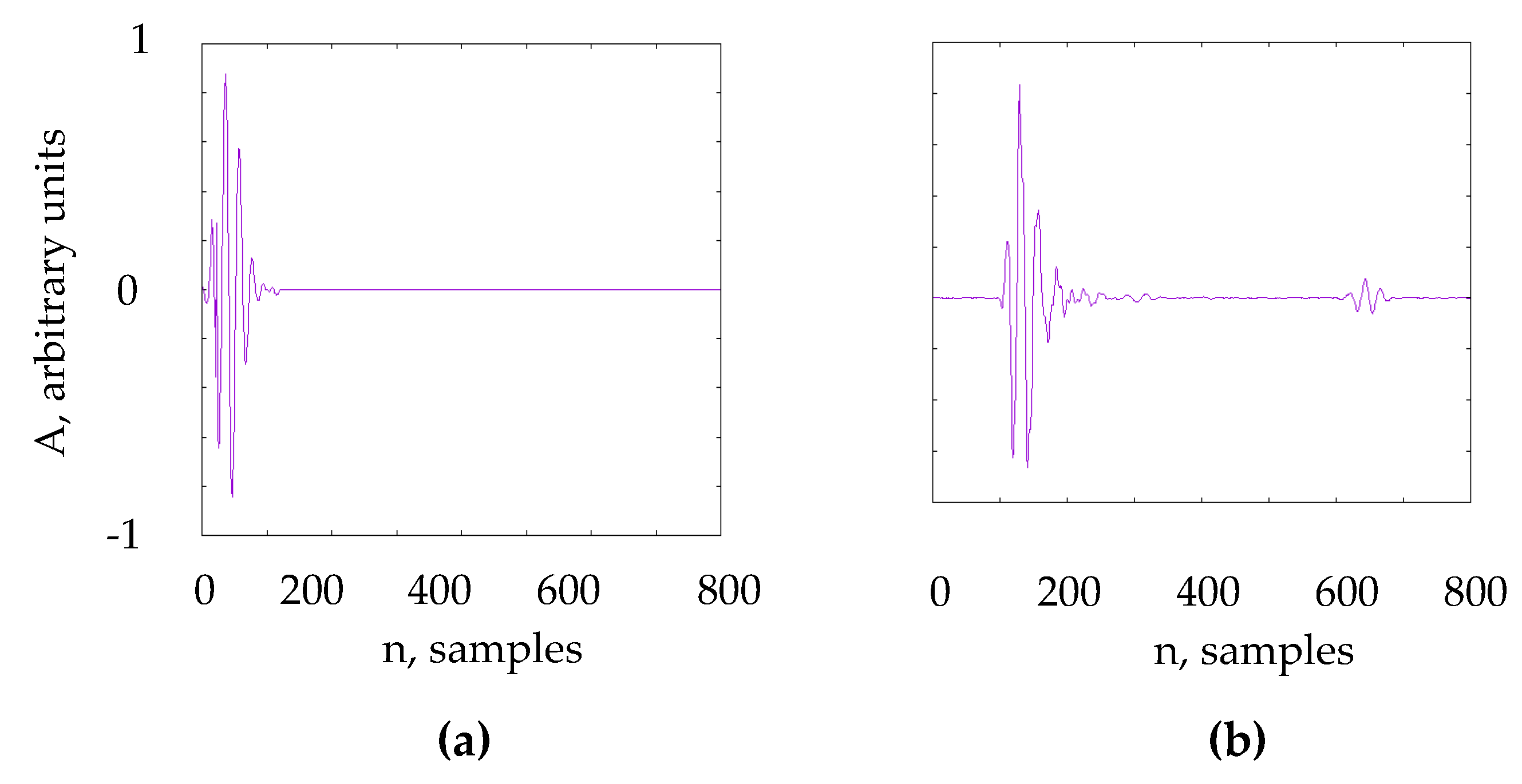
The experiments have been performed in immersion, with the water temperature of 22 °C, so that the speed in water was cw = 1.48 km/s. The water path standoff distance was about 13 mm. A typical input pulse (a pulse transmitted by a transducer) is presented in Figure 2a, and a typical A-scan (a train of pulses received at a transducer), in Figure 2b. The full matrix of A-scans, [ A k l n , k, l, = 1, 2, …, K, n = 1, …, N] has been collected, where the first index denotes the transmitter, second—the receiver and third—the time sample. Both transmitters and receivers are numbered from the left. Let us introduce t k , x , l , the time of travel from transmitter k to receiver l through one of the evenly spread nodes x = (x, z) and signal A k l ( t ) A k l n | n = t / Δ t , where Δ t is the time increment defined by the sampling frequency; t / Δ t = floor   ( t / Δ t ) . In order to reduce the processing burden [17], instead of A-scans AutoNDE uses their Hilbert transform,
h ( A k l ) ( t ) = 1 π p . v . A k l ( τ ) t τ d τ .
Note that the A-scan in Figure 2b is A 82 , 82 , n . Taking into account that the offset was n = 743 the first pulse is the echo of the pulse transmitted by element 82 arriving back to this element from the point x 1 on the upper surface of the specimen and the second pulse is the echo arriving back from point x 2 on the backwall. The distance d between x 1 and x 2 can be calculated using the standard formula d = 0.5 n cl/fs, where n is the number of time samples between arrivals of two pulses.

3. The AutoNDE Code for Semi-Automatic Crack Characterization

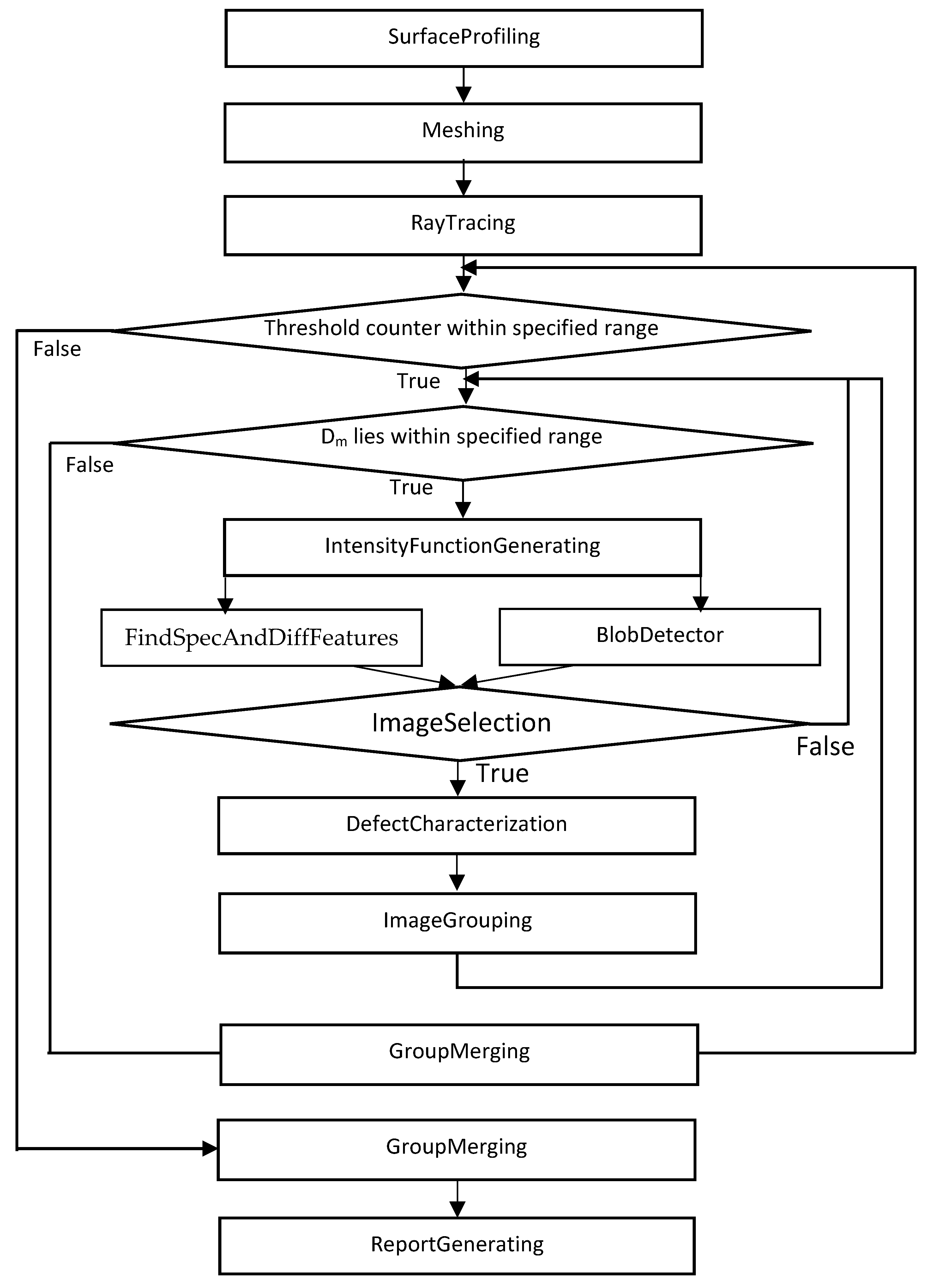
The original version of the code described in [16] was written in LabView and contained only a rudimentary AI module. In this paper we present a more advanced version written in C. Its flowchart is presented in Figure 3.
Let us describe the submodules presented there in more detail:

3.1. Signal Processing

The submodules of the Signal Processing module are used to create 2D images of the tested specimen:
  • SurfaceProfiling effects profiling by (1) locating for each array element the surface point directly underneath and (2) interpolating the acquired surface points using polynomial regression. The first step is performed by convolving h(A)(N Δ t t), the Hilbert transform of the time inverse of the input pulse with the corresponding pulse scattered by the surface. Only A-scans received by the same transducers that transmitted them are utilized. Hence the maximum number of surface points collected during the first step is K. The regression model used in interpolation is
    z = X b + e,
    where the response vector z, the parameter vector b, the design matrix X and the error vector e are given, respectively, by
    z = [ z 1 z 2 z J ] ,   X = [ 1   x 1   x 1 2     x p p 1   x 2   x 2 2     x 2 p           1   x J   x J 2     x J p ] ,   b = [ b 1 b 2 b p ] ,   e = [ e 1 e 2 e J ]
  • Originally, the polynomial degree to produce good results with the DPS data has been found by trial and error to be p = 8 .
  • In the latest version of AutoNDE the degree p is selected automatically. There is a number of approaches recommended for this purpose in the literature on machine learning. We have found that the most common of those, the bias-variance trade-off leads to ill-conditioned the Vandermonde matrix X T X and overfitting of the DPS data. Since for all DPS datasets SurfaceProfiling acquires surface points whose location error is random it is reasonable to assume that their underlying error distribution is normal. Therefore, we attempted and found satisfactory a method that involves the Wald test [18] based on the t-statistic of the leading coefficient.
  • In order to apply this method we first estimate p m a x and q m a x , where p m a x is the highest polynomial degree that can be reliably estimated from the available data and q m a x is the maximum number of digits of accuracy on top of what would be lost to the numerical method due to loss of precision from arithmetic methods [19]. A well-known rule-of-thumb suggests that p m a x = J / 5 and the training of AutoNDE on the DPS data suggests that for realistic random surface undulations used in this experiment q m a x = 6.
  • The suggested method utilizes the algorithm presented in Figure 4. Note that since all X j 2 values are non-zero and distinct for every p = p’ all Vandermonde matrices X T X are invertible [20]. Note too that the t-statistic is normally applied to assess significance of regression parameters, while here t p is used to test the null hypothesis that the leading coefficient b p = 0. It follows that the algorithm selects the polynomial of the highest significant degree. The threshold t p = 1.96 assures that if the error in location of surface points has a normal distribution, the null hypothesis that the leading coefficient is zero can be rejected at the 95% significance level.
The spline method has been tried too but was found to be too sensitive to the choice of smoothing parameters and thus not amenable to automation.
2.
Meshing of the specimen is performed by specifying a regular grid of evenly spaced rows and columns, covering the portion of the specimen, which lies underneath the probe. The meshing module also specifies the region of interest. If the measurements are taken only when the crack is located more or less underneath the array center the region of interest is reduced to the central region underneath the probe. Any reduction of the region of interest speeds up the crack characterization process.
3.
RayTracing starts by issuing a fan of rays from each array element. The central angle of each fan is −90° to the x-axis, the optimal vertex angle has been found to be 60° and the optimal difference between the angles of neighboring rays, 0.057°. These values effect a trade-off between the code accuracy and speed. For each ray the RayTracing submodule locates the point where it hits the upper surface, finds the refracted ray issuing from this point (in the current version no shadowing is accounted for) and calculates the time it takes the ray to reach each row in the region of interest. In the present version of AutoNDE mode conversion is allowed as well as one reflection from the backwall.
4.
IntensityFunctionGenerating utilizes the matrix A of A-scans to generate the intensity function
I ( x ) = | k , l h ( A k l ) ( t k , x , l ) |
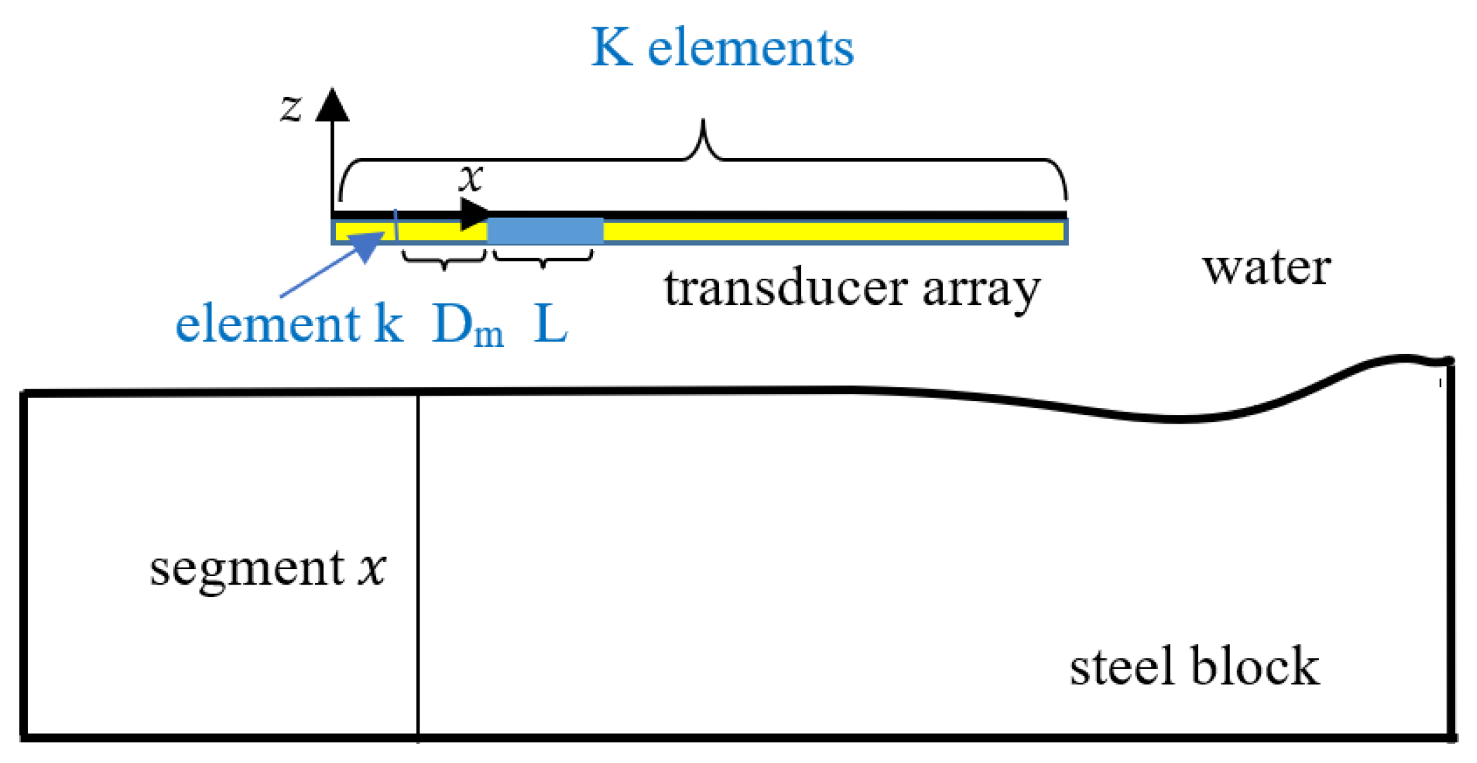
where time t k , x , l is the moment of time the corresponding pulse is at its peak. In the standard TFM (Total Focusing Method) the summation in (4) is carried out over the whole probe. In addition to TFM we use an MTFM (a Modified TFM), a signal processing approach developed by trial and error to produce not just one image for one position of the probe as in TFM but a series of images m: Inside each such image, each vertical segment x is scanned with a “partial probe” [k + Dm,k + Dm + L], k < KDmL when Dm > 0 (a blue colored portion of the transducer array in Figure 5 or [ k + DmL, k + Dm], k > LDm when Dm < 0, where the transducer element k = x / D e or k = x / D e , respectively. Here x / D e = c e i l ( x / D e ) . This allows us to use the same amount of information to image each vertical segment of the specimen, except for the segments close to the array ends. However, as a rule, the end portions of the array lie outside the region of interest. The approach often filters out the “blinding” surface reflections and enhances images of diffraction spots. Both the TFM and MTFM images are produced using the normalized version of intensity function, I 1 ( x ) = 256   I ( x ) / m a x x   I ( x ) . Each image is stored in the standard way, using 256 different intensities, the highest indicated by red color and the lowest, by blue.

3.2. Image Processing

The image processing module is used to select those MTFM images, which lend themselves to easy interpretation. The basis for selection is a priori knowledge that the crack to be characterized is large and plane. Therefore the crack image is expected to contain a straight segment, which is a specular reflection from the crack, or else two diffraction spots surrounding the crack tips. Sometimes only one crack tip can be picked up. AutoNDE differentiates the possible diffraction spots from the possible specular features by size, allowing for some overlap.
The ImageProcessing module of AutoNDE uses a variety of intensity thresholds. As mentioned above, the maximum intensity is 256. Thresholding is a standard tool in image processing, which is used to filter out noise. During the AutoNDE training, in most cases 125 has been found to produce the best results. However, some significant weak features could only be picked up at lower thresholds, while some noise could be filtered out only at thresholds that are higher. For this reason, AutoNDE normally utilizes three thresholds, 65, 125 and 185.
AutoNDE analyse the resulting images using OpenCV (Open Source Computer Vision Library) functions [21]. Two submodules are involved, FindSpecAndDiffFeatures and BlobDetector.
  • FindSpecAndDiffFeatures relies on the OpenCV FindContour function to select two types of features, large (longer than 7 mm) and small (between 1 mm and 7 mm long). If one of the features is 7 mm or slightly smaller and there are several other small features smaller than 3 mm in extent the small features are neglected and the larger one is treated as a specular reflection.
  • The BlobDetector relies on the OpenCV DetectBlob function to filter blobs by size between 80 and 160 pixels. The BlobDetector is particularly useful when dealing with surface-breaking cracks, because in these situations the probe often picks up only one crack tip. When only one blob is picked up the final crack characterization can be made only by a human inspector. In cases like this the AutoNDE flags the situation by putting the question mark after every defect characteristic and estimate of the report quality (the definition of quality is given below). All the feature and blob parameters mentioned above have been chosen by trial and error to maximize the number of true positives and minimize the number of false positives selected by the code.

3.3. Explainable AI

The AI module of AutoNDE is a decision tree, which selects images that appear to contain defects, characterizes these defects and then groups similar images. Note that by their nature, decision trees produce explainable results: all the reasoning can be traced. The decision tree comprises the following submodules:
  • ImageSelection submodule selects images containing one or two blobs (bright spots), two small contour selected features, one large feature or maybe, one blob and one small feature. If a blob and a contour selected feature are detected at the same location it is the feature parameters that are used to characterize the potential diffraction spot. If one of the contour selected features is slightly bigger than 7 mm it is still treated as a possible diffraction spot.
  • DefectCharacterization carries out calculations of the extent (notch length in the imaged plane), depth (the smallest of distances between notch tips and specimen surfaces) and orientation (the angle the notch makes in the imaged plane with the mean specimen surface) of the detected planar defect. The calculations are based on parameters of the bounding boxes, which the FindContour OpenCV function draws around the objects or else on parameters of blobs detected by the DetectBlob function. Planar cracks are expected to produce two types of images, specular reflections and TOFD (Time of Diffraction) images, which contain two diffraction spots surrounding notch tips. When the image contains one large feature (interpreted as a specular notch image), the extent is calculated as the longest box side; the depth, as the shortest distance between box vertices and specimen surfaces; and orientation as orientation of box’s longest side. For TOFD, the extent is calculated as the largest distance between vertices of their bounding boxes; the depth, as the shortest distance between vertices of these boxes and specimen surfaces; and orientation, as orientation of the line connecting the gravity centers of the boxes. If only two small features are identified the code draws a straight yellow line connecting their gravity centers.
  • ImageGrouping checks whether each selected image appears to be similar to the pivot image in the group g = 1, 2, …, G, that is contains a notch with a similar extent E and orientation O at a similar location C (so that the coordinates of the gravity centers of the notches are similar). The pivot is the image with the smallest D m in the group. If the image is similar to the pivot it is added to the group; otherwise, it is used as a pivot for the next group. The crack parameters are referred to below as v = E, O, C, respectively. For each group a preliminary report is compiled, describing the weighted averages v ¯ g .
v ¯ g = m = 1 M g w ^ g , m v g , m M ^ g ,   w ^ g , m = w e , g , m · w o , g , m · w l , g , m · w a d d ,
w v , g , m = w ( Δ v g , m ,   t v ) .
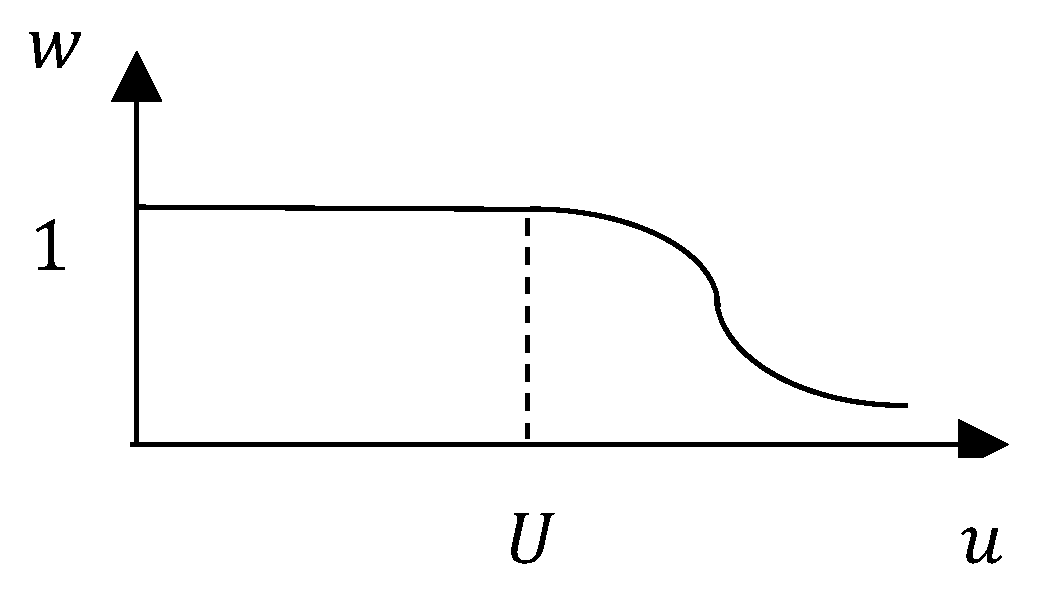
Above M ^ g = m = 1 M g w ^ g , m is a modified number of images in group g , with M g —the number of images in group; Δ v g , m = | v g , m v g , 0 | is the deviation of parameter v g , m in the group g and image m from the corresponding parameter v g , 0 in the pivot image (in case of the gravity center location, this deviation is the distance between centers); t v is the acceptable threshold for this deviation; and the weighting function, which smoothes transition over this threshold is
w ( u ,   U ) = {   1 ,   if   u < U   e ( u U 1 ) 2 ,   otherwise ,
see Figure 6. The following thresholds have been established by trial and error:
t e = t l = 2.1   mm ,   t o = 21 ° .
The weight w a d d is used to taper off the probability of almost horizontal cracks situated very close to the top surface or backwall. The quality of the resulting group report is assessed by using the subjective probability (rounded up to the nearest multiple of 10),
Q g = max { 10 % , min [ 90 % ,   100 % M ^ g M ^ ] }   ,
where M ^ = g = 1 G M ^ g is the sum of modified numbers of images in all G groups identified. Thus, one of the advantages of MTFM is the fact that various images it produces allow AutoNDE to assess the quality of crack characterization.
4.
GroupMerging employs similar principles to ImageGrouping, working with group averages instead of individual crack characteristics. Group merging is performed first for each intensity threshold: the first of all groups on the list is chosen as a pivot, the next group on the list is merged with it if the extents of their defects differ by no more than 2.1 mm; the distance between the gravity centers of these defects is no more than 2.5 mm; and their orientations differ by no more 21°. The remaining groups form a new list and the merging process is repeated. For a given intensity threshold, only groups detected by the same method (FindContour or BlobDetector) can be merged. No such restriction is used when merging groups identified using different intensity thresholds. Otherwise, this last merging is performed using the same principles as above but with deviations in extents and distances allowed to reach 3 mm.
5.
ReportGenerating reports the group(s) with the maximum probability. If more than one group with the maximum probability is reported the final choice has to be made by the human inspector on scrutinizing the TFM image.

4. Training AutoNDE

The AutoNDE was trained using sixteen datasets produced by DPS (Doosan Power Systems) and then tested on one dataset collected by AMEC and one, by CEA (The French Commission for Atomic and Alternative Energies).

4.1. Training AutoNDE on DPS Data

It has been established by trial and error that the best images of the specimen used in DPS experiment (see Figure 1) could be obtained by specifying its thickness as 29.5 mm and distance from the probe to the specimen, as 12.5 mm. In other words, it has been established that the 0.5 mm difference in these parameters has a significant effect on the image quality. The number of array elements and length of A-scan have been already specified above as K = 128 and N = 800. The optimal length of the “partial probe” has been established by trial and error to be 25 elements, covering the aperture of 20 mm. This aperture is large with respect to the typical length of the longitudinal wave: Given the longitudinal speed within the steel specimen of 5.89 km/s and the central pulse frequency of 5 MHz, this typical length is 1 mm. Similarly, it has been found that enough information could be collected with 25 images, Dm varying between 0 to 24 array elements. No interpretable images were produced for larger values of Dm. Finally, whatever the dataset, quality results have been obtained for the same region of interest. This has been chosen as the central region, roughly 20% of the area underneath the probe, symmetrical with respect to the probe center. The resulting estimates of notch characteristics are compared to their known experimental values in Table 1. The experimental values were established using standard approaches used in experiments of this nature, see, e.g., [1].
Table 1 shows that depths of the notches in DPS data could be estimated with the error of up to 2 mm (in one instance, 3 mm), and orientations—with the error of 5–10°. We note here that assuming the inspection surface plane would produce similar estimates for most of the notches but the second entry would be 7 mm in extent, located at 1 mm depth, oriented at 75° and the fourth entry would be 7 mm in extent, located at 0 mm depth, oriented at 125°. It follows that results are more reliable when small surface undulations are taken into account.
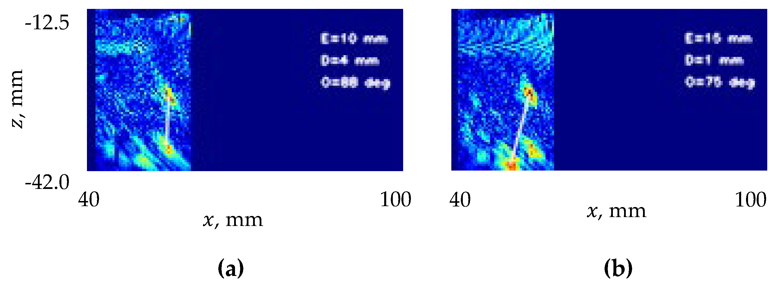
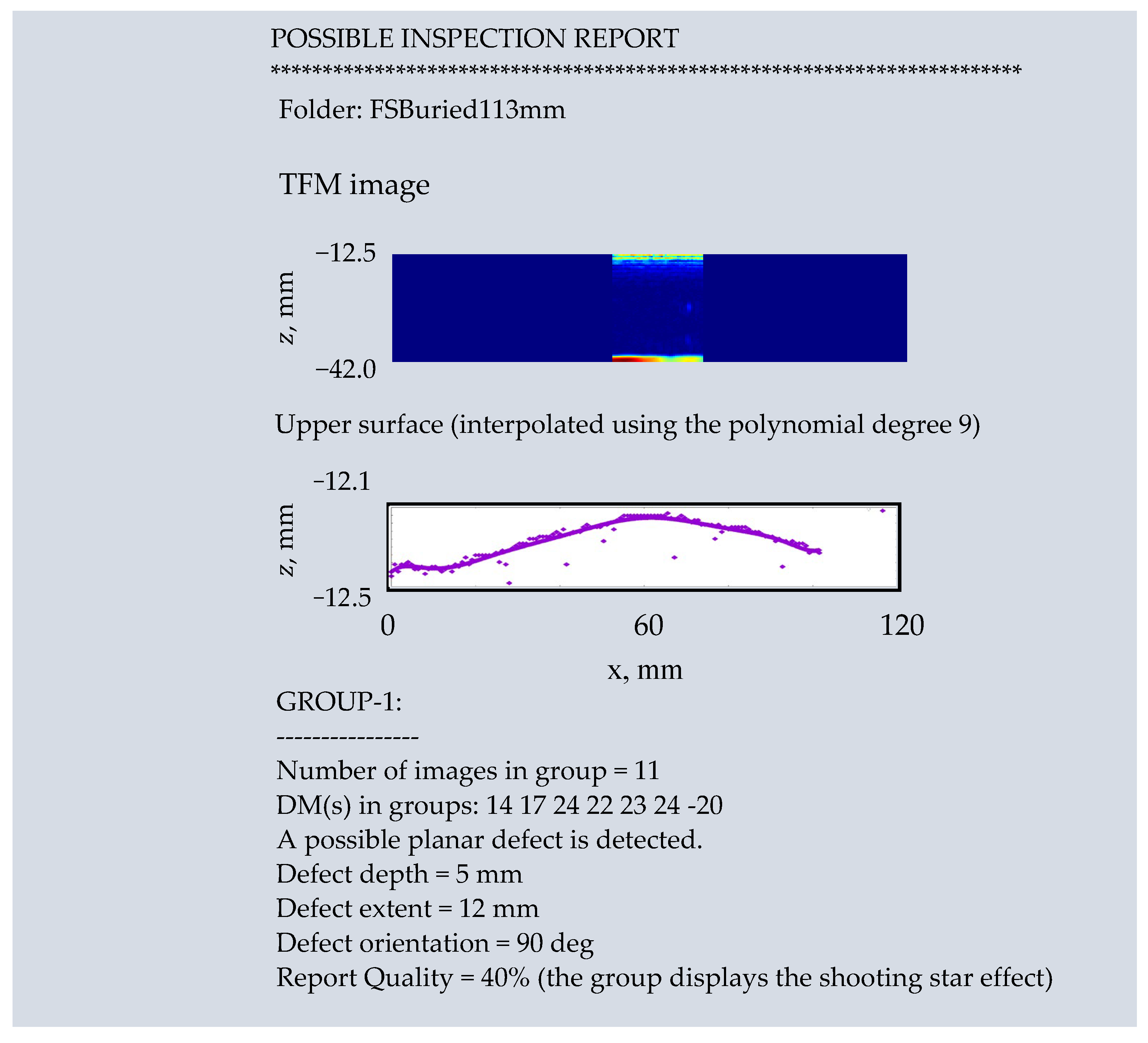
Typical MTFM images are presented in Figure 7: both Figure 7a,b contain three bright spots, with the two brightest ones joined by a thin yellow line. However, while the top spot is bright in both images, in Figure 7a the brightest lower spot is found at a distance of 4 mm from the backwall, while in Figure 7b the brightest spot lies on the backwall. We know that both bright spots in Figure 7a represent diffraction spots surrounding tips of the planar notch, while the lowest bright spot in Figure 7b is spurious, probably due to a defect in the backwall: The noise is similar to the signal and inside any given image the code cannot always distinguish between the two. However, in this case most MTFM images allow it to make the correct choice. This leads to a reasonable entry for the correponding notch in Table 1. The accompanying AutoNDE inspection report is presented in Figure 8.
Note that unlike MTFM images in Figure 7, the TFM image in Figure 8 contains bright reflections from both top surface and backwall and the portion of the image to the left of the region of interest is not cut off. Unlike with MTFM images the diffraction spots surrounding notch tips are very faint. The presence of the TFM image in the report allows a human inspector to make an immediate assessment of the validity of the AI conclusions. Note too that the upper surface points presented in the second figure of this report have been obtained using the Profiling submodule and solid line is the interpolating polynomial. Finally, the order of DMs listed in the report indicates that the first four interpretable images have been obtained with the intensity threshold of 65, the next four—with the intensity threshold of 125, and the last two—with the intensity threshold of 185.
As mentioned above, when an AutoNDE report lists several possibilities, it is for a human inspector to select the most probable. Let us illustrate this by the report for the surface-breaking notch situated 113 mm from the left edge of the specimen and inspected from the notched side. The corresponding AutoNDE report can be seen in Figure 9.
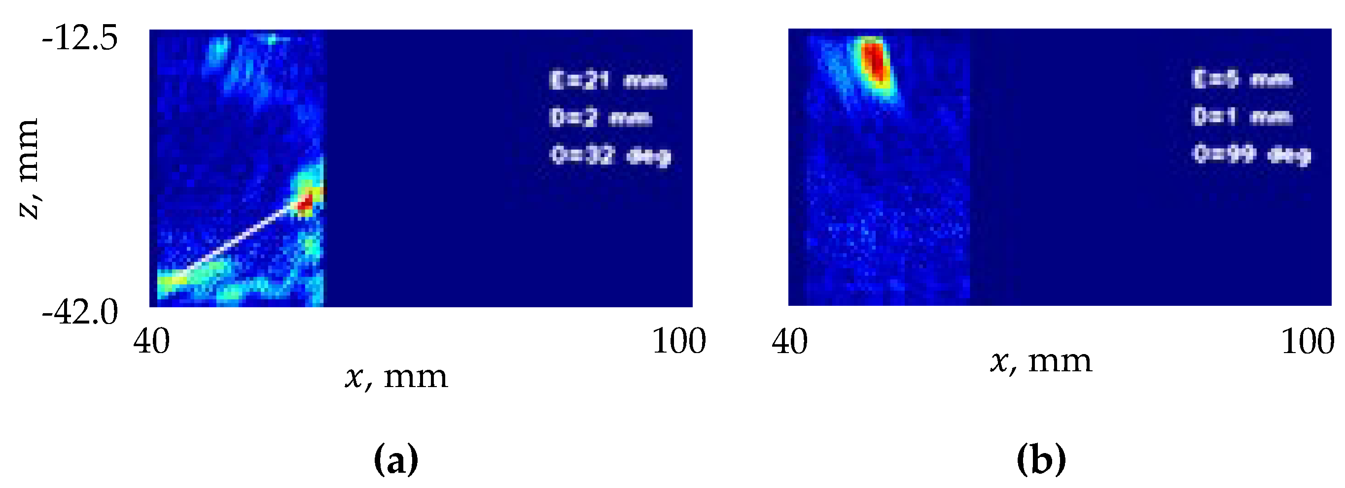
The presence of Group 1 is due to the fact that some MTFM images pick up two spurious spots, see Figure 10a. Group 2 contains slightly skewed specular images, see Figure 10b. We emphasize here that all TFM images obtained with DPS data contain either clear diffraction spots as above or else clear specular images, see Figure 11. While the present version of AutoNDE has not been trained to mask the images of upper and lower surfaces this will be done in future. It would then become possible to characterize these images without employing MTFM. Thus, the main advantage of MTFM is the fact that unlike TFM it allows to produce many images instead of one, allowing to estimate the quality of a notch image by how often it is reproduced.
Typical run times involved in creating Table 1 under the Ubuntu 64-bit operating system on the VMware workstation 16.x with an i7-1165G7 @ 2.80 GHz and 16 GB of Ram are presented in Table 2.

4.2. Testing AutoNDE on AMEC Data

AutoNDE has been tested on a data set collected by AMEC engineers using a 64 element phased transducer array with the pitch De = 0.63 mm and sampling frequency fs = 25 MHz, placed in direct contact with a 55.5 mm deep steel specimen. The geometry of the experiment, input pulse and typical A-scans are similar to the ones in the DPS experiment and are not reproduced.
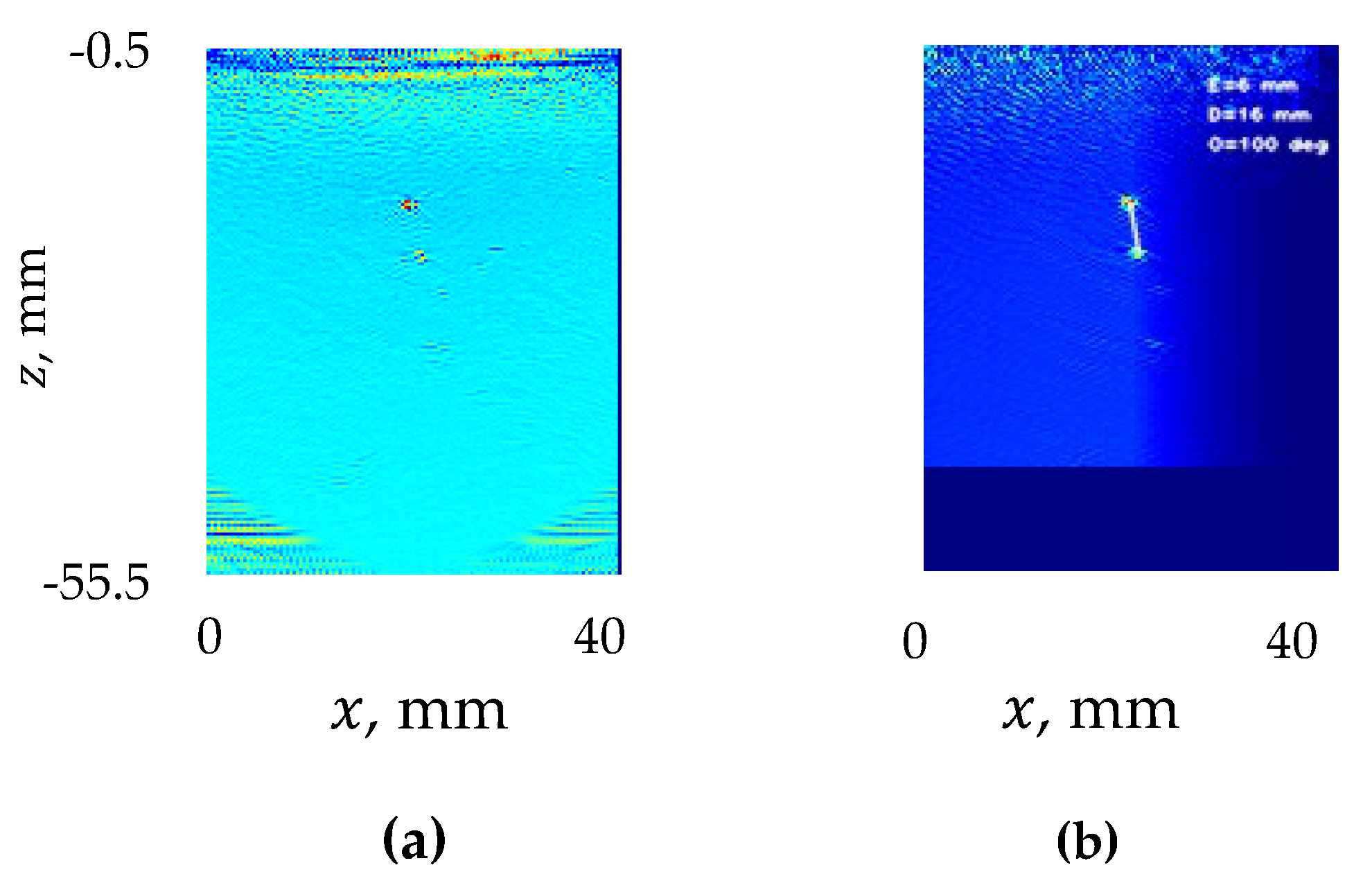
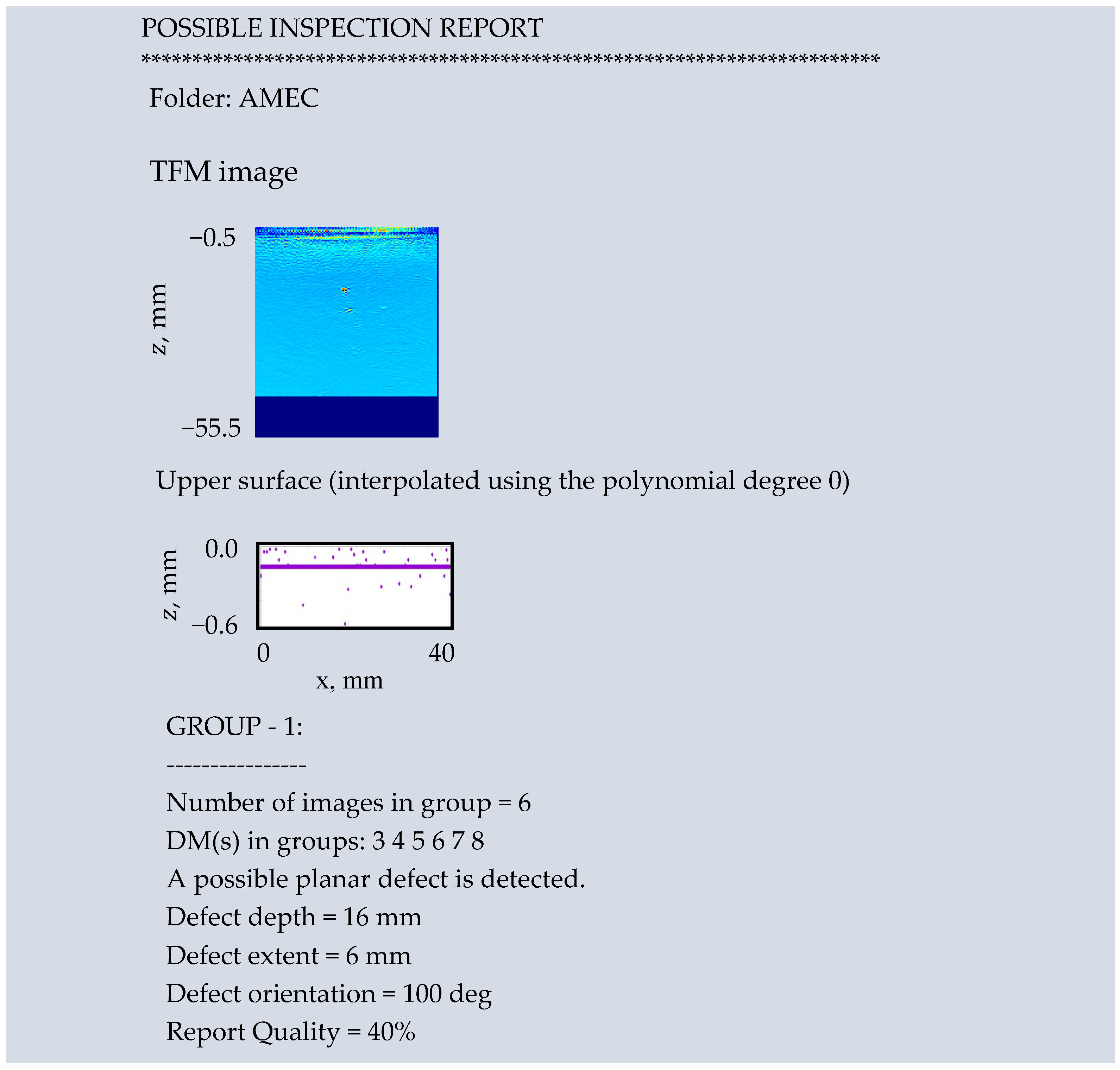
The standard TFM image of the AMEC specimen is presented in Figure 12a. It contains two diffraction spots, but they are too faint to be identified by the current version of AutoNDE. The code picks the diffraction spots up only when we cut off minimum 20% of the specimen thickness from the bottom of the image, see Figure 12b. The latter displays the following estimates of the crack characteristics: extent—4 mm, depth—16 mm, orientation —100°. The necessity to reduce the region of interest appears to be due to the defect in the backwall, which produces a response that is too bright. After the region of interest is cropped as described, AutoNDE produces the report reproduced in Figure 13. The parameters of the manufactured notch are as follows: extent—5 mm, depth—16 mm, orientation—101°. We can see that the AutoNDE estimates are of the same quality as estimates obtained with the DPS data.

4.3. Testing AutoNDE on CEA Data

AutoNDE has been also tested on a data set collected by CEA engineers using a 64 element phased transducer array, with the pitch De = 0.6 mm and sampling frequency fs = 50 MHz, imaging in immersion a 42 mm deep steel specimen. The geometry of the experiment is presented in Figure 14, the input and typical A-scans are similar to the ones in the DPS experiment and are not reproduced.
The set-up is more challenging than the one used in the DPS experiments: both the top surface and blackwall are more indulated and there is a backwall breaking flaw, creating additional response, see Figure 15b and Figure 16a. The numerical experiments conducted with CIVA [22] (a commercial package for analyzing and simulating NDT [23,24,25,26,27,28], in particular, NDT of components with irregular surfaces [7,8,28,29]) showed that the notch fabricated for the purposes of this experiment was best imaged using the half-skip LTT mode, with the L (longitudinal) transmitted pulse converting at the backwall to the T (transverse) pulse and then reflecting from the notch, so that the received pulse is also T, see Figure 16a.
Note that the CEA experiment was designed to investigate the effect of highly undulated surfaces, with the distribution of undulations different to normal. Both types of surfaces, those reproduced in the CEA experiment and those reproduced in the DPS experiment are realistic, but our analysis confirmed that they have to be modeled differently, The CIVA code was provided with precise descriptions of both the inspection surface and backwall obtained with a flexible probe. AutoNDE relied instead on a rather crude Profiling submodule described above. Moreover, the offset of 2095 samples in A-scans obtained with the 64 element transducer array was too high, eliminating reflections from the higher portions of the inspection surface. For this reason, the quality of the Profiling output was very low. A trial and error approach was used to establish that the best results could be obtained when the upper surface was assumed to be plane and the backwall was represented by a parabola, cf. Figure 15a,b with the surfaces in the AutoNDE report presented in Figure 17.
This report was obtained using the partial probe of 33 transducerelements, that is of 19.8 mm aperture. All other parameter values were the same as described in the previous sections. Inspecting the TFM image confirms that the second group provides a more reliable characterization of the 12 mm surface-breaking notch normal to the backwall. The depth is overestimated due to distortions introduced by crude of the surfaces.

5. Conclusions

A novel code containing a decision tree, that is, an explainable AI has been designed and developed for characterizing single large planar cracks. For the component surfaces whose undulation errors can be described using a normal distribution, we developed a method for automatic estimation of the degree of the interpolating polynomial. The code has been trained on 16 experimental data sets and tested on two. The inspection surface and backwall used in training had realistic small undulations whose distribuation could be considered normal. One test dataset was collected using a specimen with plane surfaces and another, a specimen with surfaces whose undulations were smooth and large and could not be described using a normal distribution.
It has been demonstrated that every type of material and inspection configuration requires preliminary investigation to establish not only how to model the surfaces but also most appropriate values of such hyperparameters as the component thickness, distance to the probe and portion of the image to be analyzed. Numerous other parameters described in this paper have been optimized manually. Remarkably, they perform well on all datasets described in the paper. It is important to realize that in some configurations only one crack tip can be picked up and in others no crack localization is possible.
Once suitable parameters and limitations are established the code can be used to generate possible inspection reports. These contain an assessment of their own quality based on the subjective probability of the report being correct. The probabiltiy is calculated by analysing a variety of images (rather than one) produced by a particular modification of the TFM offered in this paper. It is expected that the human inspectors would still have to examine the AutoNDE reports, particularly the TFM images they contain, to ascertain whether they agree with the preliminary conclusions made by the AI module.
Despite the initial success reported here, just like any other artificial intelligence system, the code can be guaranteed to analyze well only the type of data used for its training, so that, say, the random undulations of the component surface follow the same probability distribution as in the training data set. Also, so far AutoNDE has been trained to process only the regions of interest, which contain one crack or else several cracks parallel to the inspection surface. It is clear that many more data sets are required for testing AutoNDE before it is accepted by the NDT community as a practical tool. To widen the AutoNDE applicability we have plans to automate the choice of the hyperparameters described above too. It is also clear that other methodologies have to be developed for modeling surfaces with undulations that do not obey a normal distribution. Notwithstanding these challenges, AutoNDE shows a great promise, demonstrating feasibility of an explainable AI, suitable for applications in industrial NDE, increasing its accuracy and efficiency.

Author Contributions

Conceptualization, methodology, validation, writing, supervision, project administration, funding acquisition, L.F.; software, S.U.A. and L.F.; data interpretation, review and editing, M.D. All authors have read and agreed to the published version of the manuscript.

Funding

The research was supported by the Innovate UK grants nos. 131671, 132928 and 2553 as well as the EURIKA/Innovate UK grant no 106151.

Data Availability Statement

Restrictions apply to the availability of these data. Data was obtained from Doosan Power Systems, AMEC and CEA are available from L.F. with the permission of these organisations.

Acknowledgments

The authors are grateful to the Innovate UK monitoring officers Tom Harris and Chris Marshall for their critical feedback and constant support and to the colleagues from the Ultrasonics and NDT group, Bristol University for providing the AMEC data and Sébastien Robert for the CEA data acquisition. They are also grateful to Nicolas Pignet, who undertook translation of the original LabView code into C when a second year ENSEIRB-MATMECA engineering student seconded under the Internship Agreement to Sound Mathematics Ltd., funded by a European Union Erasmus grant. Finally the authors would like to thank anonymous reviewers for many helpful suggestions on improving the presentation of the paper.

Conflicts of Interest

The authors declare no conflict of interest.

References

  1. Schneider, C.; Bird, C. Reliability of Manually Applied Phased Array Inspection. In Proceedings of the 4th European-American Workshop on Reliability NDE, Berlin, Germany, 24–26 June 2009. [Google Scholar]
  2. Hunter, A.J.; Drinkwater, B.W.; Wilcox, P.D. Least-squares estimation of imaging parameters for an ultrasonic array using known geometric image features. IEEE Trans. Ultrason. Ferroelectr. Freq. Control. 2011, 58, 414–426. [Google Scholar] [CrossRef]
  3. Marengo, E.A.; Gruber, F.K.; Simonetti, F. Time-Reversal MUSIC Imaging of Extended Targets. IEEE Trans. Image Process. 2007, 16, 1967–1984. [Google Scholar] [CrossRef] [PubMed]
  4. Champagnat, F.; Goussard, Y.; Idier, J. Unsupervised deconvolution of sparse spike trains using stochastic approximation. IEEE Trans. Signal Process. 1996, 44, 2988–2998. [Google Scholar] [CrossRef] [Green Version]
  5. Holmes, C.; Drinkwater, B.W.; Wilcox, P. Advanced post-processing for scanned ultrasonic arrays: Application to defect detection and classification in non-destructive evaluation. Ultrasonics 2008, 48, 636–642. [Google Scholar] [CrossRef] [PubMed]
  6. Hunter, A.J.; Drinkwater, B.W.; Wilcox, P. The wavenumber algorithm for full-matrix imaging using an ultrasonic array. IEEE Trans. Ultrason. Ferroelectr. Freq. Control. 2008, 55, 2450–2462. [Google Scholar] [CrossRef] [PubMed]
  7. Iakovleva, E.; Chatillon, S.; Bredif, P.; Mahaut, S. Multi-mode TFM imaging with artifacts filtering using CIVA UT forwards models. AIP Conf. Proc. 2014, 1581, 72–79. [Google Scholar] [CrossRef]
  8. Le Jeune, L.; Robert, S.; Villaverde, E.L.; Prada, C. Plane Wave Imaging for ultrasonic non-destructive testing: Generalization to multimodal imaging. Ultrasonics 2016, 64, 128–138. [Google Scholar] [CrossRef] [Green Version]
  9. Bannouf, S.; Robert, S.; Casula, O.; Prada, C. Noise filtering in the total focusing method by decomposition of the time reversal operator and the virtual array approach. AIP Conf. Proc. 2013, 1511, 857–864. [Google Scholar] [CrossRef]
  10. Villaverde, E.L.; Robert, S.; Prada, C. Ultrasonic imaging of defects in coarse-grained steels with the decomposition of the time reversal operator. J. Acoust. Soc. Am. 2016, 140, 541–550. [Google Scholar] [CrossRef]
  11. Robert, S.; Casula, O.; Roy, O.; Neau, G. Real-time nondestructive testing of composite aeronautical structures with a self-adaptive ultrasonic technique. Meas. Sci. Technol. 2013, 24, 074011. [Google Scholar] [CrossRef]
  12. Pyle, R.J.; Rhodri, L.T.; Bevan, R.R.; Hughes, R.K.; Rachev, A.A.S.A.; Wilcox, P.D. Deep Learning for Ultrasonic Crack Characterization in NDE. IEEE Trans. Ultrason. Ferroelectr. Freq. Control 2021, 68, 1854–1865. [Google Scholar] [CrossRef] [PubMed]
  13. Bai, L.; Le Bourdais, F.; Miorelli, R.; Calmon, P.; Velichko, A.; Drinkwater, B.W. Ultrasonic Defect Characterization Using the Scattering Matrix: A Performance Comparison Study of Bayesian Inversion and Machine Learning Schemas. IEEE Trans. Ultrason. Ferroelectr. Freq. Control. 2021, 68, 3143–3155. [Google Scholar] [CrossRef] [PubMed]
  14. Shipway, N.; Huthwaite, P.; Lowe, M.; Barden, T. Using ResNets to perform automated defect detection for Fluorescent Penetrant Inspection. NDT E Int. 2021, 119, 102400. [Google Scholar] [CrossRef]
  15. Nageswaran, C. The Snooker Algorithm for Ultrasonic Imaging of Fatigue Cracks in order touse Parameter-Spaces to Aid Machine Learning. Preprints 2021, 2021070269. [Google Scholar] [CrossRef]
  16. Fradkin, L.; Zernov, V.; Elston, G.; Taneja, R.; Bell, I.; Lines, D.; Wharrie, J.; Fitzgerald, P.J. Towards semi-automated crack characterisation. J. Phys. Conf. Ser. 2013, 457, 012008. [Google Scholar] [CrossRef] [Green Version]
  17. Badeau, N.; Painchaud-April, G.; Le Duff, A. Use of the Total Focusing Method with the Envelope Feature. Available online: https://www.olympus-ims.com/en/resources/white-papers/use-of-the-total-focusing-method-with-the-envelope-feature/ (accessed on 1 November 2021).
  18. Fahrmeir, L.; Kneib, T.; Lang, S.; Marx, B. Regression: Models, Methods and Applications; Springer: Berlin, Germany, 2013. [Google Scholar]
  19. Cheney, W.; Kincaid, D. Numerical Mathematics and Computing, 7th ed.; BROOKS/COLE Sengale Learning: Boston, MA, USA, 2013. [Google Scholar]
  20. Macon, B.; Spitzbart, X. Inverses of Vandermonde Matrices. Am. Math. Mon. 1958, 65, 95–100. [Google Scholar] [CrossRef]
  21. Home—OpenCV. Available online: https://opencv.org (accessed on 1 November 2021).
  22. Available online: http://www.extende.com/ (accessed on 1 November 2021).
  23. Mahaut, S.; Chatillon, S.; Darmon, M.; Leymarie, N.; Raillon, R.; Calmon, P. An Overview of Ultrasonic Beam Propagation and Flaw Scattering Models in the Civa Software. AIP Conf. Proc. 2010, 1211, 2133–2140. [Google Scholar]
  24. Toullelan, G.; Raillon, R.; Chatillon, S. Results of the 2013 UT modeling benchmark obtained with models implemented in CIVA. AIP Conf. Proc. 2014, 1581, 2093–2100. [Google Scholar] [CrossRef] [Green Version]
  25. Raillon-Picot, R.; Toullelan, G.; Darmon, M.; Calmon, P.; Lonné, S. Validation of CIVA Ultrasonic Simulation in Canonical Configurations. In Proceedings of the 18th World Conference on Non-destructive Testing (WCNDT), Durban, South Africa, 16–20 April 2012. [Google Scholar]
  26. Raillon, R.; Bey, S.; Dubois, A.; Mahaut, S.; Darmon, M. Results of the 2010 Ut Modeling Benchmark Obtained with Civa: Responses of Backwall And Surface Breaking Notches. AIP Conf. Proc. 2011, 1335, 1777–1784. [Google Scholar] [CrossRef]
  27. Raillon, R.; Bey, S.; Dubois, A.; Mahaut, S.; Darmon, M. Results of the 2009 Ut Modeling Benchmark Obtained with Civa: Responses of Notches, Side-drilled Holes and Flat-bottom Holes of Various Sizes. AIP Conf. Proc. 2010, 1211, 2157–2164. [Google Scholar] [CrossRef]
  28. Ferrand, A.; Darmon, M.; Chatillon, S.; Deschamps, M. Modeling of ray paths of head waves on irregular interfaces in TOFD inspection for NDE. Ultrasonics 2014, 54, 1851–1860. [Google Scholar] [CrossRef] [PubMed] [Green Version]
  29. Darmon, M.; Dorval, V.; Baqué, F. Acoustic Scattering Models from Rough Surfaces: A Brief Review and Recent Advances. Appl. Sci. 2020, 10, 8305. [Google Scholar] [CrossRef]
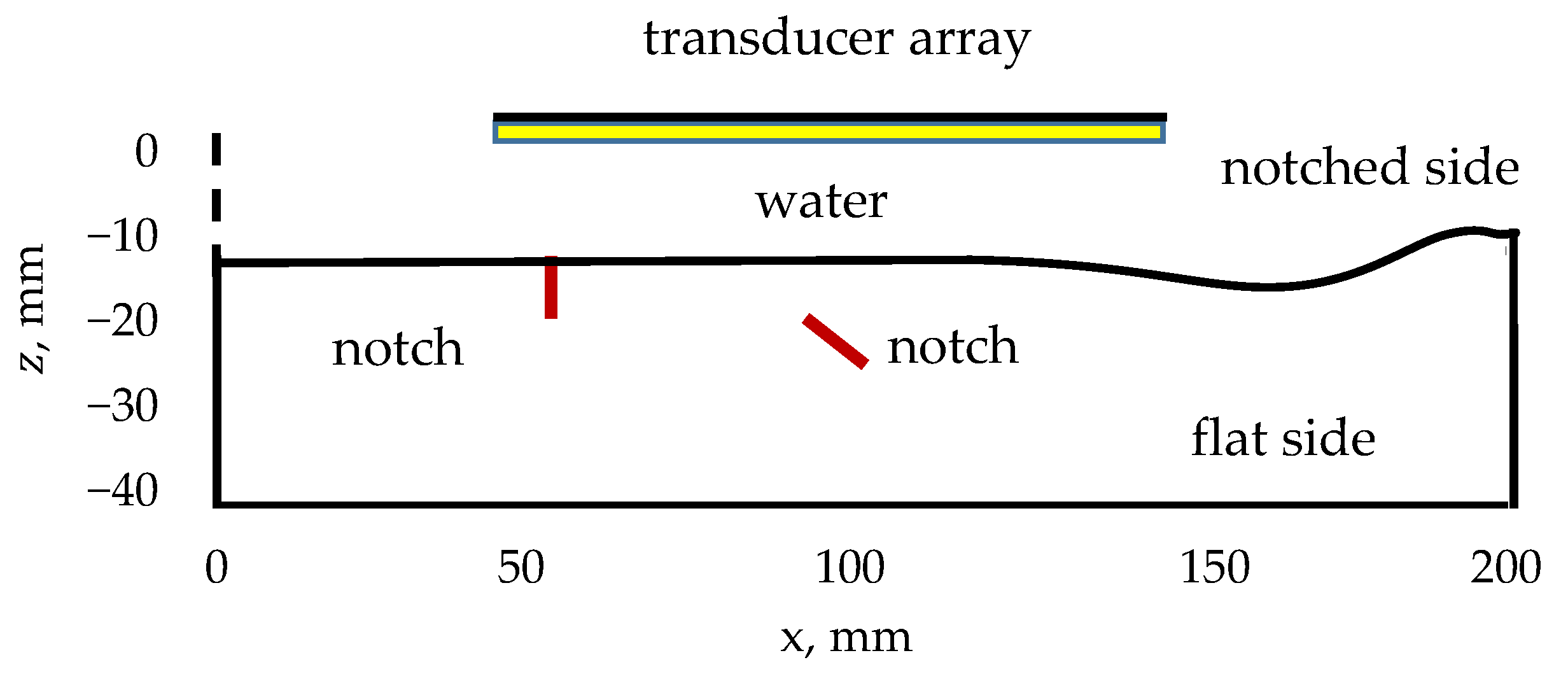
Figure 1. A schematic of the DPS experiment.
Applsci 11 10867 g001
Figure 2. (a) A typical input pulse A_n; and (b) a typical A-scan A_n.
Applsci 11 10867 g002
Figure 3. A flowchart of AutoNDE.
Applsci 11 10867 g003
Figure 4. An algorithm for automatic identification of the interpolating polynomial.
Applsci 11 10867 g004
Figure 5. A schematic of MTFM.
Applsci 11 10867 g005
Figure 6. Modification weights.
Applsci 11 10867 g006
Figure 7. DPS data set: the buried notch located 113 mm from the left edge, imaged from the flat side. MTFM images have been obtained with intensity threshold = 185 and Dm = (a) 24; (b) 21. Key: E—notch extent, D—notch depth and O—notch orientation. The portion of the image to the left of the region of interest is cut off.
Applsci 11 10867 g007
Figure 8. Inspection report for buried notch located 113 mm from the left edge. Key (here and below): dots–surface points acquired by SurfaceProfiling; line interpo lating polynomial.
Applsci 11 10867 g008
Figure 9. Inspection report for the surface-breaking notch located 113 mm from the left edge.
Applsci 11 10867 g009
Figure 10. The DPS data set: the surface-breaking notch located 113 mm from the left edge, imaged from the notched side. MTFM images have been obtained with (a) intensity threshold = 125, Dm = −11, and (b) intensity threshold = 185, Dm = 15. Key as in Figure 7.
Applsci 11 10867 g010
Figure 11. The DPS data set: the TFM image of the surface-breaking notch (circled) located 70 mm from the left edge, imaged from the notched side. Key as in Figure 7.
Applsci 11 10867 g011
Figure 12. The AMEC data set. (a) The standard TFM image of the full specimen; (b) an MTFM image, with 20% thickness cut off the bottom, intensity threshold = 125, Dm = 3.
Applsci 11 10867 g012
Figure 13. The inspection report for the AMEC dataset.
Applsci 11 10867 g013
Figure 14. A schematic of the CEA experiment.
Applsci 11 10867 g014
Figure 15. CEA experimental specimen. (a) The upper surface and (b) the backwall.
Applsci 11 10867 g015
Figure 16. CEA data set. The backwall notch imaged with a 64 element transducer array, using the half-skip LTT mode as processed by (a) CIVA and AutoNDE, (b) employing the standard TFM algo-rithm and (c) MTFM (intensity threshold = 185 and Dm = −8).
Applsci 11 10867 g016
Figure 17. The inspection report for the CEA dataset.
Applsci 11 10867 g017
Table 1. The DPS data set: Estimated (est) and experimental (exp) crack characteristics. The crack position is specified as distance between the notch and left edge of the specimen. The “hc” stands for Human Choice and indicates that the estimates are chosen by a human and not the AI.
Inspection Surface/
Approximate Notch Depth/
Notch Distance from Edge
Report
Quality/Comments
Defect Parameters
Extent,
in mm Est/Exp
Orientation, in deg
Est/Exp
Depth,
in mm
Est/Exp
Flatside/Buried/24 mm60%9/10105/1108/5
Flatside/Buried/62 mm40%6/5105/1105/5
Flatside/Buried/113 mm40%12/1090/905/5
Flatside/Buried/149 mm20%hc5/585/906/5
Flatside/Breaking/25 mm60%6/580/900/0
Flatside/Breaking/64 mm90%11/1090/900/0
Flatside/Breaking/113 mm60%7/5100/1100/0
Flatside/Breaking/150 mm90%12/10110/1101/0
Notchside/Buried/24 mm60%11/10110/1105/5
Notchside/Buried/62 mm70%6/5110/1105/5
Notchside/Buried/113 mm30%12/1090/904/5
Notchside/Buried/149 mm30%5/580/903/5
Notchside/Breaking/25 mm40%5/5100/901/0
Notchside/Breaking/70 mm30%hc8/1090/902/0
Notchside/Breaking/113 mm30%5/5115/1101/0
Notchside/Breaking/155 mm50%8/10115/1102/0
Table 2. Maximum run times (in seconds) involved in creating Table 1.
Reading DataProfilingRaytracingCreating an ImageI/O HandlingTotal
1.5221.5412
Publisher’s Note: MDPI stays neutral with regard to jurisdictional claims in published maps and institutional affiliations.