Article

Dual Head and Dual Attention in Deep Learning for End-to-End EEG Motor Imagery Classification

1
Center for Digital Media Computing, Informatices School, Xiamen University, 422 Siming South Road, Xiamen 361005, China
2
Computer and Science School, Minnan Normal University, Xiang Qianzhi Street 36, Xiangcheng District, Zhangzhou 363000, China
3
OYMotion Technologies Co., Ltd., Floor 6, Building 2, 222 Guangdan Road, Shanghai 201318, China
*
Author to whom correspondence should be addressed.
Appl. Sci. 2021, 11(22), 10906; https://doi.org/10.3390/app112210906
Submission received: 24 September 2021 / Revised: 5 November 2021 / Accepted: 8 November 2021 / Published: 18 November 2021

Abstract

:
Event-Related Desynchronization (ERD) or Electroencephalogram (EEG) wavelet is essential for motor imagery (MI) classification and BMI (Brain–Machine Interface) application. However, it is difficult to recognize multiple tasks for non-trained subjects that are indispensable for the complexities of the task or the uncertainties in the environment. The subject-independent scenario, where an inter-subject trained model can be directly applied to new users without precalibration, is particularly desired. Therefore, this paper focuses on an effective attention mechanism which can be applied to a subject-independent set to learn EEG motor imagery features. Firstly, a custom form of sequence inputs with spatial and temporal dimensions is adopted for dual headed attention via deep convolution net (DHDANet). Secondly, DHDANet simultaneously learns temporal and spacial features. The features of spacial attention on each input head are divided into two parts for spatial attentional learning subsequently. The proposed model is validated based on the EEG-MI signals collected from 54 subjects in two sessions with 200 trials in each sessions. The classification of left and right hand motor imagery in this paper achieves an average accuracy of 75.52%, a significant improvement compared to state-of-the-art methods. In addition, the visualization of the frequency analysis method demonstrates that the temporal-convolution and spectral-attention is capable of identifying the ERD for EEG-MI. The proposed machine learning structure enables cross-session and cross-subject classification and makes significant progress in the BMI transfer learning problem.

1. Introduction

Motor imagery (MI) classification based on electroencephalogram (EEG) event-related synchronization (ERS) and event-related desynchronization (ERD) phenomena is a measure of the neuron extent when people image body movements [1,2,3,4].
In recent years, two typical and general approaches make important achievements in EEG-MI recognition and brain–machine interface (BMI): optimizing the hand-crafted features and extracting the ERS/ERD features by deep learning. For the former approach, common spatial pattern (CSP) filters and Riemannian Manifold [5,6,7,8] are two popular and effective methods. The CSP method is optimal for discrimination of the filtered time series data, and it forms a low dimensional spatial-subspace for the acquired multi-channel EEG data and derives a covariance matrix for each MI class [9]. Guan’s group introduced Filter Bank Common Spatial Pattern (FBCSP) as an extension of the original CSP algorithm and gained attention by winning the 2008 BCI Competition IV-2a [10,11]. The FBCSP algorithm recognized that not all frequency bands contain discriminative information, and it optimized the data-driven spectral filter and spatial filter. The Riemannian based dimension reduction algorithm is derived to construct a low-dimensional embedding from high-dimensional Riemannian manifold. Li’s group used the geodesic distance of Riemannian manifold to determine the adjacency and weight in Riemannian graph, and then proposed bilinear regularized locality preserving (BRLP) to address the problem of high dimensions frequently arising from BMIs [6]. Ref. [7] proposed Riemannian distance and Riemannian mean was directly adopted to extract tangent space (TS) features from spatial covariance matrices of the MI EEG trials. Researchers in [12] utilized a scheme for transfer learning to use the Riemannian geometry of symmetric and positive definite(SPD) matrices, tightly connected to the BMI transfer learning work. Ref. [13] proposes a time-frequency decomposition-based weighted ensemble learning (TFDWEL) method, which aims to improve the classification performance of motor imagery EEG signals. In recent years, EEG power topography is used for MI classification [14,15].
However, few of these methods are subject-independent explorations. There are currently a number of approaches targeting the subject-independent EEG signal analysis via machine learning. In this area, several studies had made progress via CNN (Convolutional Neural Network). Sakhavi et al. [16] combined multiple one-versus-rest CSP features on CNN for multi-classes MI classification. In [17], a 3D representation is generated by transforming EEG signals into a sequence of 2D arrays which preserve spatial distribution of sampling electrodes. Then, the work proposed a multi-branch 3D CNN and a corresponding classification strategy to preserve temporal-spatial features. In [18], a Convolutional Recurrent Attention Model (CRAM) is built to encode the EEG signals and a recurrent attention mechanism is proposed to explore the temporal dynamics of the EEG signals. Majoros et al. [19] recognized 10 volunteers MI activities with a feedforward, multi-layer perceptron network and convolutional neural network in combination with different data pre-processing methods. In addition, one dimension-aggregate approximation is also employed to extract effective MI signal representation for long short-term memory (LSTM) networks, such as [20,21]. In [21], not only the time and frequency domain features but also a Random Forest (RF) was used to evaluate feature weights.
Fields like Natural Language Processing (NLP) and even computer vision have been revolutionized by the attention mechanism. Recent advances in interpreting deep model behaviors, including the employment of attention mechanism [18,21,22] and utilization of several types of inputs from frequency or time domain or both, have significantly enhanced the classification accuracy. However, to the best of our knowledge, the cross-task and cross-subject classification is still challenging.
Deep ConvNets [9] and EEGNet [23] can be applied to MI classification [17,18,24], P300 detection [25,26], workload estimation [27,28,29], and error- or event-related potential decoding [30], and they become common approaches to learn the selective preprocessed handcraft data. The work in [9] followed a famous method of FBCSP [10] to construct the input data and then trained the data onto CNN with known training features. In particular, Ref. [24] improved performance via a semi-supervised contrastive learning framework with two different networks based on Deep ConvNets and EEGNet. However, the unknown features and/or structures for training need to be explored. Another popular approach is building 3D CNN structures with different sizes of receptive field [17]. Though the multi-branch structure performs better than one branch network, the computational cost grows proportionally with the number of the branches. This is a common problem with complex CNN models which result in more training time and worse real-time performance. In addition, LSTM and RNN also have the same disadvantage since they are slower and take up more memory than other normal activation functions, such as sigmoid, tanh, or rectified linear unit. To handle this problem, Conv1D is selected to learn the temporal features. Thus far, there are many papers based on temporal-spectral features for EEG classification, which have achieved good results, such as [27,31].
However, the existing CNN-based classification methods depend on a single convolution computation, which limits the classification accuracy. In this work, we desire to exploit valuable intermedia learning signals to enforce the feature value. Two attention mechanisms for temporal and spatial learning are proposed to improve the accuracy of EEG MI classification.
In this work, a dual-attention convolution network is proposed to handle subject-independent recognition of MI actions. First, the raw EEG data are filtered by bandpass filter. Then, the time serialized data are divided into segments of equal length. Finally, the dual blocks of deep learning in CNN structure are utilized to learn temporal and spatial-spectral EEG representations. To enhance the learning ability of the MI features and improve the accuracy of EEG MI classification, two attention mechanisms are utilized to enforce the temporal and spatial-spectral characteristics respectively. The block diagram of the proposed DAC-Net framework is shown in Figure 1.
For a comparable analysis of the role of deep 1D and 2D design choices in EEG-MI decoding, three key questions are addressed:
-
What’s the impact on the proposed attention strategy through end-to-end learning?
-
How to quantify or visualize the interpretability of deep DAC-Net?
-
How to accelerate the learning manifestation and effectiveness from the MI raw signals via DAC-Net for BMI recognition applications?
The remainder of this paper is organized as follows: Section 2 introduces the experiment data. Section 3 describes the preprocessing of EEG signals and the overall architecture of DAC-Net. Section 4 presents experiment results and evaluates the performance of the proposed method. Section 5 describes the interference with data acquisition, as well as providing the visualization of the learned features. Finally, Section 6 concludes this paper.

2. Data

The MI-EEG dataset [32] utilized in this research was recorded by the department of brain and cognitive engineering, Korea University, which is shortened as KU-MI dataset. Fifty-four healthy subjects (ages 24–35; 25 females) participated in the experiment. All of them had no history of neurological, psychiatric, or any other pertinent disease that otherwise might affect the experimental results. Thirty-eight subjects were naive BMI users and the others had previous experience of BMI experiments.
For all blocks of this MI-EEG paradigm, the first 3 s of each trial began with a black fixation cross that appeared at the center of the monitor to prepare subjects for the MI task. Afterwards, the subject performed the imagery task of grasping at the appropriate hand for 4 s after the right or left arrow appeared as a visual cue. The MI experiment consisted of training and test phases; each phase had 100 trials with balanced right and left hand imagery tasks. Hence, 21,600 (54 subjects × 2 sessions × 200 tails) trials segmented from the continuous training and testing data can be fetched.
EEG signals were recorded at a sampling rate of 1000 Hz and collected with 62 Ag/AgCl electrodes. The EEG amplifier used in the experiment was a BrainAmp (Brain Products; Munich, Germany). The data were obtained from 20 MI cortices [33,34,35] of FC1-6, C1-6, CP1-6, Cz, and FPz (see Figure 2).

3. Method

In this section, we discuss the main components of our method. First, we design a dual-input preprocessing method (Section 3.1). Next, we exploit two custom attention mechanisms respectively for temporal and spatial feature extraction (Section 3.2). Finally, we discuss how we train our model from the dual-input EEG (Section 3.3). Figure 3 contains an overview of our method.

3.1. Input Data

In this work, a trial-wise strategy evaluating two approaches to defining is adopted. The input examples and the corresponding labels are identical to the cropped extracted samples. As shown in Figure 4, the first input is earlier than the second input according to the configured time parameter which is called transferring time in milliseconds. Since different EEG electrodes reflect the electrical fluctuations of different brain areas, there are strong relations between different EEG electrodes [36]. Thus, small local filtering has limited abilities to explore the important spatio-temporal representation of EEG signals. A cropped training strategy was exploited to handle the EEG data by presenting the input as a 2 D —array with the number of window sizes as the width and the electrode number on the MI area as the height.
The corresponding crop label is utilized as a target to train the DAC-Net. Such a generic architecture was selected for three reasons: first, to cover event-related desynchronization (ERD) or event-related energy (ERE) features, the window sizes of EEG data are cropped to 3000 ms that are introduced in Section 5. Second, the structure of the input data was fit for learning temporal-spatial features and the data were intercepted to 1000 ms. Meanwhile, 1100 ms of previous data was fetched to apply to the standard DAC-Net as a general-purpose tool for brain signal tasks in real time. For example, if the stride step time and transferring time are 100 ms, and the time sizes are 1100 ms, 600 segment data could be obtained from each subject session data, as 3 segments × 200 tails.
Training ERD/ERS examples are inherently sequential, which contains many features as longer sequence lengths. However, the memory and/or GPU used in the experiment limit the processing of BMI in real time. To overcome this problem, the raw data are down sampled to remove jitters by setting the trigger timing to a sampling rate of 256 Hz and band-pass filtering at 4∼40 Hz. Down-sampling the data helps to increase the output speed of each electrode, but in order to achieve real-time processing, it should be avoided. For a given group (training or testing), all data were loaded into a single three-dimensional Numpy array. The dimensions of the array are [samples, ime steps, channels], or rather [ N i , 400 , 34 ] , which maps the total sample number from ten-folder-cross subjects, 400 records, and 34 channels.
We built a set of crops with crop size T as time slices of the trial: C j = X S , W , F , E j , where S is the segmental sample number, W is the data window size, F is the number of frequency bands with 22 in this paper, and E is the number of electrodes on 20 MI areas were selected. All of these C j crops are new training data examples of our decoder and will have the same label y j as the original trail.
Crops were collected starting on trial cue, with the last ending of 4 s after the cue ends. Overall, this resulted in 3100 crops and label predictions per trial for each subject. D i = x 1 , y 1 , x 2 , y 2 , , x N i , y N i , where N i denotes the total number of cropped data onto subject i. The input matrix x j R T × E of cropped j, 1 j N i contains the preprocessed signals of E-recorded electrodes and T-discretized time steps recorded per window size. In addition, the number of samples, i = 1 l e n ( s u b s ) k = 1 N S ( r i , e i k , w , s ) , is the total number of cropped in any given raw signal data files.

3.2. Attention Module

Attention is the process of reinforcing behavior and cognition by selectively focusing on a discrete aspect of information and ignoring other perceived information. Attention mechanisms have become part of compelling sequence modeling and transduction models in various tasks, allowing the modeling of dependencies regardless of their distance between the input sequence and the output [37]. For MI recognition, a suitable attention model can be applied to new users without pre-calibration in the subject-independent scenario [38]. The attention model of action recognition/detection helps to improve the judgment on actions that occur in MI by focusing on specific relevant signals in the spatial–spectral–temporal domain.
In this paper, the spatial-spectrum-temporal dual attention is introduced to two steps, which learns different focusing weights for different ERD in the temporal dimension and different focusing weights for different EEG channels in the spatial dimension, see Figure 3. Before elaborating the spatial-spectrum-temporal attention(SSTA), the basic notations are presented first:
ψ t X 1 , X 2 = φ i , j | φ i , j = S o f t m a x X 1 · X 2 d 2 · X 2
The input EEG sequence is denoted as X, which defines X t and X s in the processes of temporal learning and spatial learning, respectively. The SSTA module attempts to learn the attention W weighting the spectrum in temporal and spatial dimensions. In addition, an attention function ψ · is defined for the SSTA module, which learns the weights W from the input features X. Based on ψ , the output sequence Y generated by passing X through the SSTA module can be defined. In the next part of this paper, subscripts t and s are used to distinguish X , W , ψ , Y at the temporal or spatial learning level. Figure 3 shows the whole SSTA network module.
The principles of the SSTA module are as follows:
  • The module is as simple and efficient as possible, relying on the combined operation of convolution, pooling, normalization, and anti-overfitting.
  • The module has robust and nonlinear learning capabilities by enabling 1D CNNs in the temporal dimension and 2D CNNs in the spatial dimension.
  • This module conducts attention learning in the temporal dimension firstly, which helps to improve the subsequent spatial dimension learning (see Section 5.1).

3.2.1. Key-Value Attention Mechanism

The key value attention was originally used by Daniluk et al. to separate the data structure and maintain a separate vector for the attention calculation [37]. The ERD/ERS signal phenomenon in the time dimension is focused first. After three-dimensional one-dimensional convolution, maximum pooling, normalization, and dropout encoding, the generalized characteristics of the dual input data are obtained. Based on the global correlation, the data characteristics are strengthened through the learning of the key value attention mechanism. This process mainly learns the spectral characteristics of the time domain, referred to the TSA (Temporal-Spectrum-Attention) module. In the learning process of the TSA module, the softmax function is used to activate X t 2 to capture the enhanced information of the corresponding feature map from X t 1 . This algorithm adopts the strategy of inductive migration and the difference between dual input data. The data characteristics of task relevance are utilized to narrow the scope for searching features.
The information on the hidden layer is referred to as “feature map” to distinguish it from the input data. According to the difference in each feature map, the output feature weight vector is represented as W t . Suppose the input information is X t i ( 0 ) = x j , k R T × E , i [ 1 , 2 ] , where T is the time window of the divided time window with downsampling. For example, if the segmentation window is 3 s and the downsampling frequency is 250 Hz, then T is 768; E is the number of the collection MI electrode leads. The Temporal Spectrum Module (TSM) can learn the dynamic weight distribution W t i = w j , k R L × F , i [ 1 , 2 ] , where L Is the number of features in the time dimension, and F is the number of output filters in the upper convolutional layer. The transfer attention layer adopts the dual input values X t 1 ( 11 ) and X t 2 ( 11 ) , which are abbreviated as X 1 and X 2 in the following formula. The algorithm function of the key value attention mechanism is defined as Equation (1), where i and j are the two dimensions of X, d 2 is the dimension of the input weight X t i matrix, and ψ t is the R B × D matrix. For the visualization of key value attention, the time-dimension eigenvalue changes of the input eigenvalues X 1 , X 2 and the output value ψ t in each layer of the filter are captured, see Section 5.1 for details.

3.2.2. Spatial Attention

After converting the EEG 1D eigenvalues to the 2D spatial spectrum tensor X s , the intermediate features are weighted by the Conv2D encoder, and then the self-attention calculation is performed, as the second step shown in Figure 3. This mainly learns the acquisition, and the spectral characteristics of the joint electrode space are referred to as SSA (Temporal-Spectrum-Attention) module. The self-attention mechanism was first proposed by IBM and applied to the hidden layer of the bidirectional LSTM [39]. The self-attention mechanism extracts the features of sparse data onto convolution and pooling, which has been widely used in natural language processing, especially machine translation. After calculating through the attention mechanism, the dependence on external features is reduced, and the correlation between internal features of the data [40] is strengthened.
The last TSA module can distinguish time changes and strengthen the characteristic information of ERD/ERS. Each lead information is processed independently. The spectral characteristics of the spatial dimension hide the unlearned features in the network. One problem in this process is how to convert the 1D EEG feature map composed of multiple leads into a 2D structure conforming to the spatial information. In this case, their spatial spectrum characteristics can be learned. To handle this problem, the input data onto EEG electrodes is arranged in symmetrical order for the collected electrodes from front to back, from left to right. Meanwhile, before conducting the feature learning of the self-attention mechanism, the features of the TSA module are output first. The quantity is converted to the input tensor X s 0 = x i j k R B 0 × R × C of the SSA module, where B is the number of output feature maps; R, C are the 1D feature values converted to 2D tensors Reconstruction coefficient, R × C = D ; D is the last channel dimension of the output characteristic value of the TSA module. The convolution calculation is performed again, which is equivalent to the initial learning of the feature value of the spatial dimension, and the distribution weight is recalculated.
The self-attention mechanism algorithm of the SSA module combines two hidden functions. First, according to the difference of each characteristic value X s , the weight distribution vector of the characteristic difference is calculated. The calculation process follows the softmax activation function H X j which is R B 4 × R × C matrix, as exhibited in Equation (2). The maximum pooling is used to learn each feature map H and feature weight W to capture the feature information between each lead electrode.
ψ s X = H = h i j k | h i j k = e x i j k l = 1 C e i j l G W · H

3.3. DHDANet

The Dual Head Dual Attention (DHDANet) model includes three parts, as shown in Figure 3:
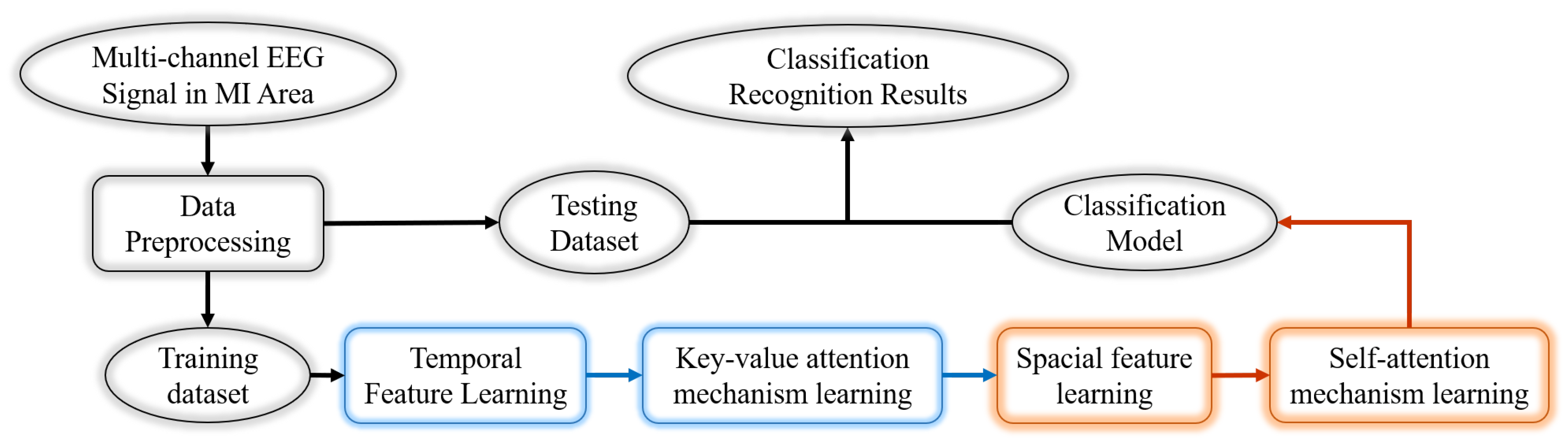
  • TSA module: As for the characteristics of ERD/ERS phenomenon, the input heads perform three sets of time-domain wave amplitude feature learning. Each set of time-domain training includes one-dimensional convolution, maximum pooling, data normalization, and dropout operation. Then, the Key-value attention learning is performed, and the feature values of the dual input head correspond to the key and value in the attention mechanism. The three sets of time-domain feature extraction parameters are the same. It mainly performs neighborhood filtering. The parameter set and processing process of the network are shown in Figure 5. First, one-dimensional convolution is performed to extract different feature maps with a core of 32 and a time interval of 0.128s (32/250) because the down-sampling rate is 250 Hz. Then, MaxPool 1D continues. At this time, the learning processes volatility characteristic value at a time interval of 0.25s. Data normalization and dropout are conducted to prevent overflow and overfitting [41,42]. After three sets of time-domain features are extracted, each feature map covers 1s of EEG waveform feature information, and from the analysis in Section 3.1, the time period for an ERD/ERS peak or trough is generally between 500 ms to 1s [43,44]. It can be seen that, before entering the key-value attention calculation, a peak or trough of ERD/ERS exists in the two input feature maps.
  • SSA module: After extracting the feature value of time domain, this module focuses on extracting the spectral features in spatial domains of the left and right hemisphere. For feature extraction in the spatial domain, the amplitude information of the ERD/ERS phenomenon cannot be extracted for convolution calculation that is too short or too long. In particular, if the triple feature extraction is performed on the input data of the network initially, the convolution and maximum pooling are used. The further reduction of computing will result in the loss of valuable information, which cannot be used for action recognition. To avoid this problem, the SSA module in this chapter first converts the 1D feature values output by the TSA module into a 2D tensor with a 4-column structure, Conv2D = (2,2), so that the symmetrical lead signals of the two brain regions can be convolved to calculate the weight of the feature map. Before and after the self-attention calculation, convolution and dropout calculations are added. This former is to obtain dynamic weights based on the feature information to prepare for self-attention calculations. In addition, the latter is to compress feature values to facilitate the calculation of the next module, as shown in Figure 6.
  • Feature classification learning module: This module is to classify the temporal and spatial features learned in the training network and build a classifier. This module uses two fully connected layers, and the basic operation of fully connected is the matrix vector product. The first completely connected layer of the module aims to weight the probability of the existence of each neuron feature. After common machine learning operations with unique data and over-fitting, the second fully connected layer classifies the feature weights output by the previous connected layer absolutely.
Each training cycle of the DHDA net uses the Nadam activation function, which has a certain range and a Nesterov momentum term for the learning of each iteration, making the parameters more stable and the learning rate more restrictive. In addition, a direct effect on updating the gradient is imposed by this function. Inspired by algorithms such as FBCSP [10,11,45] and SBLFB [46], two frequency bands including 8–20 Hz and 20–30 Hz are used to build a DHDA model, according to the law of motor imagery.

4. Experiments and Results

The DHDANet network has two key points. Firstly, the input data contain event-related desynchronization (ERD) or Event-related energy (ERE) function; secondly, the spatial feature is retained in the process from a one-dimensional temporal feature map to a two-dimensional structure. In addition, a two-dimensional nonlinear calculation algorithm is performed, and the parameters must be appropriate for extracting the features.
The experimental results and the advantages of the proposed method in the end-to-end model of EEG across subjects are shown in this section. The data acquisition method of the dual-input mechanism is exhibited first. The effectiveness and advantages of using the attention mechanism algorithm based on the dual-input in the time domain and the spatial domain are then proved. Finally, the comparison of DHDANet to the best method in the literature is based on the classification performance through the data collection on the KU-MI data set.
All experiments are implemented with Python and Tensorflow running on an NVIDIA GTX 1080 Ti GPU.

4.1. Data PreProcessing

This experiment includes two stages of training and testing (or two sessions). In each stage, imagine the left and right hand grasping actions 100 times. Therefore, the KU-MI data set has a total of 21,600 samples generated by 54 subjects × 2 sessions × 100 times of each MI action × 2 types of MI actions.
According to the data segmentation strategy in Section 2, the sliding step λ = 100 ms, and the time window of the input training EEG signal is 3 s. Due to dual inputs, the interval between the front and back is 100 ms, and the actual information segmentation window is ω = 3100 ms. 4 s of motion image and nine input samples can be divided each time, so there are 194,400 experimental samples in total. It is sufficient to analyze the reliability of these samples with confidence, and the results will be shown in Section 5.1.
This paper aims to realize an end-to-end machine learning model and an online brain–computer interaction interface, and the data preprocessing supports real-time data collection. TensorFlow and Keras are used in this work to build a DHDA learning network. In the training process, the learning rate and batch size of DHDA are set to 0.001 and 1024, respectively. For this data preprocessing strategy, the cluster-level statistical permutation is tested. Figure 7 shows the statistics result about the left hand MI action corresponded to the right in the C3, Cz, and C4 electrodes. The result calculated with permutations and cluster-level correction(see Figure 7) shows that the max distinguishing point is at 3.5 s.

4.2. Result

According to the analysis in Section 2, the input data finally used in this chapter comes from: down-sampling rate of 250 Hz, band-pass filter at 4 to 40 Hz, extraction of KU-MI data from 20 acquisition points in the motor imaging area, and intercepting induced events according to the law of ERD/ERS. The data in the next 2 to 6 s is based on a time window of 3 s, a step length of 100 ms, and double input. Meanwhile, the latter input is delayed by 100ms than the previous one. This paper uses ten-fold crossed validation which is loaded from an component of sklearn package.model_selection KFold to test the performance of the DHDA model and compare it with the other four methods. Before the training of each model, the input data are randomly mixed, and the training data and test data are distributed at a ratio of 9:1. The learning rate is 0.001 and training is performed iteratively 100 times. The strategy for saving the model in training is as follows:
  • Validation loss rate must be lower than the previous iteration before this model is saved.
  • If the test loss rate of the trained model does not decrease within 30 iterations, the training is automatically stopped.
The batch size of the DHDA model is 512, and it is trained 393 times in each Epoch. The learning process of the model is exhibited in Figure 8. Generally, after 60 times of iterative training, the accuracy of the test no longer changes, but the loss value still increases, indicating an overfitting. The suite of hyper parameters in DHDANet’s and the superiority of the model algorithm can be verified.
The proposed algorithm is compared with the four methods on the KU-MI data set, all of which use ten-fold cross-validation. Among them, CSP-cv [32] uses the CSP algorithm. The team introducing CSP-cv is also the designer and data collector of the KU-MI data set experimental paradigm, marking the subjects in the KU-MI data set as the first. There are 33 people who performed the motor imagery experiment of this experimental paradigm at one time (generally inexperienced subjects will have poorer quality in completing the specified tasks); Deep ConvNet [47] and EEGNet [23] both use a compact for EEG Shallow ConvNet. The former is designed as a general architecture, not limited to specific functional types, and the latter model is as parameterized as possible. Both models can be used to classify and identify classification tasks of different brain–computer interface paradigms. In addition, FBCNet [48] performs a heuristic convolutional neural network based on the neurophysiology of motor imagery.
Since CSP-cv is not subject to an end-to-end machine learning, it is used as a reference method for the other end-to-end learning methods. Based on the experimental results shown in Table 1, FBCNet and DHDANet are better than CSP-cv. The DHDANet model used in this work achieves 2.08% higher average classification accuracy than the latest FBCNet. Moreover, compared with the other four algorithms, DHDANet has a high recall rate, indicating that the recognition rate of poor samples is satisfactory. Meanwhile, the speciality is also high, indicating a low false positive rate for samples with non-motor imagery. DHDANet has high sensitivity and specificity for MI recognition, which confirms the superiority and is a popular choice for high performance diagnostics.

5. Analysis and Discussion

In this section, we prove the advantage of DHDANet by comparing the recognition effect with or without our custom attention (Section 5.1). Then, we put forward the next step of our work based on this work (Section 5.2).

5.1. Why Use the Attention Mechanism Algorithm?

In order to verify the effectiveness of the dual-input dual-attention mechanism algorithm for the recognition and classification of motor imagery machines, five network frameworks are built in this work through the combination of “single or dual input” and “with or without an attention mechanism learning module”. The frameworks are shown in Figure 9, where NAF means no attention framework; SAF means only self-attention framework; DAF means dual (transferring and self) attention framework; TAF means only transferring attention framework.
The experimental results of these frameworks are shown in Figure 9, and the statistical results of classification accuracy are shown in Table 2. The order from low to high is: SHNA→SHSA→SHDA→DHTA→DHDA. Comparing the result of SHDA and DHDA, it can be seen that the dual-input mechanism has 8.89% higher accuracy, indicating a significant improvement in the classification and the necessity of dual-input. Based on the comparison between SHNA and DHTA, the key-value attention mechanism in the dual-input time domain contributes to 6% higher classification accuracy, showing the necessity of a key-value attention mechanism in the time domain. Comparing between SHDA and SHSA, it can be seen that the classification accuracy of the self-attention mechanism in the airspace increases by 1.36%, verifying the necessity of the self-attention mechanism. In addition, the classification accuracy continues to increase by 7.53% by adding double input. The analysis shows that it is necessary to first learn from the time domain to strengthen the ERD/ERS characteristics of the airspace.
From the comparison of pre- and post-calculation of key-value attention feature maps with SHSA and SHDA in Figure 9, it can be seen that the key-value attention algorithm enables the ERD/ERS feature to strengthen the main features and weaken the unnecessary features. Meanwhile, it is helpful for subsequent SSA model learning because this attention mechanism reinforced the features.
The classification effect of Lee et al. [32] on the KU-MI data set marked by novices (as shown in Figure 10 subject ID circled in red) and non-beginners is further analyzed through statistical analysis of the box line between the two shown in Figure 11a. There is much more clutter for the non-MI illiteracy subjects to do the MI experiment, and this indicates the superiority of DHDANet in the extraction of generalizable features and proves that DHDANet has higher performance. The DHDANet model achieves more concentrated classification accuracy for non-initialists than other algorithms, and it obtains the highest average value. This shows that the brain–computer interface implemented with the DHDANet model for repeated users has better stability. The classification accuracy of the DHDANet model for the beginners is shown in Figure 11b. The distribution concentration and average accuracy are second to CSP-cv and FBCNet, respectively. This result shows that the subjects’ brains are not fixed and the machine interaction application scenario has a high recognition rate and stability.

5.2. Feature Works

In order to realize an end-to-end cross-subject brain–computer interaction, the similarity feature can be searched before the identification is performed and submitted in real time. Bai et al. [49] proposed an adaptive similarity metric, which is consistent with k nearest neighbor search, an original similarity function used as the kernel function to calculate the hash code to achieve fast search. Inspired by the self-hashing method [50], the EEG data are retrieved through a hash retrieval algorithm, and similar data are stored in the corresponding hash sets. When the data are represented by a high-dimensional vector, the hash operation is usually used as an effective solution for similar search. Hash search and bash search are two methods that can be tried to improve EEG similarity feature search [51,52]. In addition, the number of selecting MI electrodes has an impact on the dimension of learning data structure and speed of training. For this, we will conduct research on an automatic electrode selection method [53] in future work.
As for learning the focusing weights for different frames in the temporal dimension and different channels in the spatial dimension, some biological research gives us a good idea, such as [54] extract and learning a set of informative features from a pool of support vector machine-based models trained using sequence-based feature descriptors. In addition, ref. [55] used a feature representation learning strategy that automatically learns the most discriminative features from existing feature descriptors in a supervised way, which can improve the performance for action recognition and detection tasks on EEG. Additionally, We plan to use predictive tools to select predictive features that will help find the most effective [56]. There are benefits for BCI researchers to use control strategies and conduct the interactive feedback applications [57].

6. Conclusions

This paper proposed a neurophysiologically motivated DHDANet architecture for classification of motor imagery EEG data. While being completely interpretable, the proposed architecture offered a significant increase of +2.08% in classification accuracy. DHDANet is based on the two-level attention model from brain waves. The features of the ERD/ERS and the frequency spectrum through the temporal and spatial feature are learned by DHDANet. Experimental results showed that DHDANet can outperform the best methods in the literature. Three innovations are made in this work:
  • To learn the ERD/ERS features in the time domain, double-input EEG data are used. Meanwhile, the features are handled by the key value attention mechanism. Experimental results confirm that the key value attention mechanism is beneficial for both the recognition of motor imagery in the time domain and the follow-up learning of spatial EEG characteristics.
  • Clever conversion methods are used to transform time domain features to spatial domain features. In addition, the EEG collection point information input into the network is combined into a two-dimensional matrix according to front-back and left-right symmetry in the brain area, to retain characteristics of the left and right brain activities when handling a three-dimensional matrix conversion.
  • In the spatial feature learning module, a reasonable nonlinear computer system is constructed to extract features. In addition, a self-attention mechanism algorithm is introduced to further strengthen the features of motor imagery in the spatial dimension, see the comparison of the before and after feature maps of the key-value attention calculation in b and c in Figure 12.
In addition, the proposed method only needs to be fine-tuned according to different paradigms before it can be applied to the classification and recognition of different types of features, reducing the calibration time in actual use. This algorithm is suitable for multi-classification tasks such as intra-subject motor imagery, and enhances the generality of classification.

Author Contributions

Conceptualization, J.Y.; Formal analysis, M.X.; Investigation, M.X. and H.N.; Methodology, M.X.; Resources, J.Y.; Supervision, J.Y.; Validation, H.N.; Visualization, H.N.; Writing—original draft, M.X. and H.N.; Writing—review and editing, M.X. All authors have read and agreed to the published version of the manuscript.

Funding

This work is supported by the National Nature Science Foundation of China (No. 62072388), the collaborative project fund of Fuzhou-Xiamen-Quanzhou Innovation Zone (No.3502ZCQXT202001), the industry guidance project foundation of Science Technology Bureau of Fujian province in 2020 (No.2020H0047), the Natural Science Foundation of Science Technology Bureau of Fujian province in 2019 (No.2019J01601), the creation fund project of Science Technology Bureau of Fujian province in 2019 (No.2019C0021), the president fund of Minnan Normal University in 2021 (No.L22137).

Institutional Review Board Statement

Not applicable.

Informed Consent Statement

Not applicable.

Data Availability Statement

The data presented in this study are available on request from the corresponding author.

Acknowledgments

The authors thank all members of the Center for Digital Media Computing and the BCI laboratory at Xiamen Universiy for their discussions and inspiration. Furthermore, many thanks are due Cuntai Guan from Nanyang Technological University for his valuable advice.

Conflicts of Interest

The authors declare no conflict of interest.

References

  1. Nagai, H.; Tanaka, T. Action Observation of Own Hand Movement Enhances Event-Related Desynchronization. IEEE Trans. Neural Syst. Rehabil. Eng. 2019, 27, 1407–1415. [Google Scholar] [CrossRef]
  2. Crk, I.; Kluthe, T.; Stefik, A. Understanding Programming Expertise: An Empirical Study of Phasic Brain Wave Changes. ACM Trans. Comput.-Hum. Interact. 2015, 23, 2–29. [Google Scholar] [CrossRef]
  3. Tariq, M.; Trivailo, P.M.; Simic, M. Detection of knee motor imagery by Mu ERD/ERS quantification for BCI based neurorehabilitation applications. In Proceedings of the 11th Asian Control Conference (ASCC), Gold Coast, QLD, Australia, 17–20 December 2017. [Google Scholar]
  4. Tang, Z.; Sun, S.; Zhang, S.; Chen, Y.; Li, C.; Chen, S. A brain–machine Interface Based on ERD/ERS for an Upper-Limb Exoskeleton Control. Sensors 2016, 16, 2050. [Google Scholar] [CrossRef] [Green Version]
  5. Xie, X.; Yu, Z.L.; Gu, Z.; Li, Y. Classification of symmetric positive definite matrices based on bilinear isometric Riemannian embedding. Pattern Recognit. 2019, 87, 94–105. [Google Scholar] [CrossRef]
  6. Xie, X.; Yu, Z.L.; Gu, Z.; Zhang, J.; Cen, L.; Li, Y. Bilinear Regularized Locality Preserving Learning on Riemannian Graph for Motor Imagery BCI. IEEE Trans. Neural Syst. Rehabil. Eng. 2018, 1, 698–708. [Google Scholar] [CrossRef]
  7. Chu, Y.; Zhao, X.; Zou, Y.; Xu, W.; Song, G.; Han, J.; Zhao, Y. Decoding multiclass motor imagery EEG from the same upper limb by combining Riemannian geometry features and partial least squares regression. J. Neural Eng. 2020, 17, 046029. [Google Scholar] [CrossRef]
  8. Yger, F.; Berar, M.; Lotte, F. Riemannian approaches in Brain-Computer Interfaces: A review. IEEE Trans. Neural. Syst. Rehabil. Eng. 2017, 25, 1753–1762. [Google Scholar] [CrossRef] [PubMed] [Green Version]
  9. Kwon, O.Y.; Lee, M.H.; Guan, C.; Lee, S.W. Subject-Independent Brain-Computer Interfaces Based on Deep Convolutional Neural Networks. IEEE Trans. Neural Netw. Learn. Syst. 2019, 31, 3839–3852. [Google Scholar] [CrossRef] [PubMed]
  10. Ang, K.; Zheng, Y.; Zhang, H.; Guan, C. Filter Bank Common Spatial Pattern (FBCSP) in Brain-Computer Interface. In Proceedings of the 2008 IEEE International Joint Conference on Neural Networks (IEEE World Congress on Computational Intelligence), Hong Kong, China, 1–8 June 2008; pp. 2390–2397. [Google Scholar]
  11. Ang, K.; Chin, Z.; Wang, C.; Guan, C.; Zhang, H. Filter bank common spatial pattern algorithm on BCI competition IV datasets 2a and 2b. Front. Neurosci. 2012, 6, 39. [Google Scholar] [CrossRef] [PubMed] [Green Version]
  12. Zanini, P.; Congedo, M.; Jutten, C.; Said, S.; Berthoumieu, Y. Transfer Learning: A Riemannian geometry framework with applications to Brain-Computer Interfaces. IEEE Trans. Biomed. Eng. 2018, 65, 1107–1116. [Google Scholar] [CrossRef] [Green Version]
  13. Zheng, L.; Ma, Y.; Li, M.; Xiao, Y.; Feng, W.; Wu, X. Time-frequency decomposition-based weighted ensemble learning for motor imagery EEG classification. In Proceedings of the 2021 IEEE International Conference on Real-time Computing and Robotics (RCAR), Xining, China, 15–19 July 2021; pp. 620–625. [Google Scholar]
  14. TK, M.J.; Sanjay, M. Topography Based Classification for Motor Imagery BCI Using Transfer Learning. In Proceedings of the 2021 International Conference on Communication, Control and Information Sciences (ICCISc), Idukki, India, 16–18 June 2021; Volume 1, pp. 1–5. [Google Scholar]
  15. Xu, M.; Yao, J.; Zhang, Z.; Li, R.; Zhang, J. Learning EEG Topographical Representation for Classification via Convolutional Neural Network. Pattern Recognit. 2020, 105, 107390. [Google Scholar] [CrossRef]
  16. Sakhavi, S.; Guan, C.; Yan, S. Learning temporal information for brain-computer interface using convolutional neural networks. IEEE Trans. Neural Netw. Learn. Syst. 2018, 29, 5619–5629. [Google Scholar] [CrossRef]
  17. Zhao, X.; Zhang, H.; Zhu, G.; You, F.; Kuang, S.; Sun, L. A Multi-branch 3D Convolutional Neural Network for EEG-Based Motor Imagery Classification. IEEE Trans. Neural Syst. Rehabil. Eng. 2019, 27, 2164–2177. [Google Scholar] [CrossRef] [PubMed]
  18. Zhang, D.; Yao, L.; Chen, K.; Monaghan, J. A Convolutional Recurrent Attention Model for Subject-Independent EEG Signal Analysis. IEEE Signal Process. Lett. 2019, 26, 715–719. [Google Scholar] [CrossRef]
  19. Majoros, T.; Oniga, S. Comparison of Motor Imagery EEG Classification using Feedforward and Convolutional Neural Network. In Proceedings of the IEEE EUROCON 2021—19th International Conference on Smart Technologies, Lviv, Ukraine, 6–8 July 2021; pp. 25–29. [Google Scholar]
  20. Wang, P.; Jiang, A.; Liu, X.; Shang, J.; Zhang, L. LSTM-Based EEG Classification in Motor Imagery Tasks. IEEE Trans. Neural Syst. Rehabil. Eng. 2018, 26, 2086–2095. [Google Scholar] [CrossRef] [PubMed]
  21. Zhang, G.; Davoodnia, V.; Sepas-Moghaddam, A.; Zhang, Y.; Etemad, A. Classification of Hand Movements from EEG using a Deep Attention-based LSTM Network. IEEE Sens. J. 2019, 20, 3113–3122. [Google Scholar] [CrossRef] [Green Version]
  22. Zhang, D.; Yao, L.; Chen, K.; Wang, S. Ready for Use: Subject-Independent Movement Intention Recognition via a Convolutional Attention Model. In Proceedings of the 27th ACM International Conference on Information and Knowledge Management (CIKM), Torino, Italy, 22–26 October 2018; pp. 1763–1766. [Google Scholar]
  23. Lawhern, V.J.; Solon, A.J.; Waytowich, N.R.; Gordon, S.M.; Hung, C.P.; Lance, B.J. EEGNet: A Compact Convolut- ional Neural Network for EEG-based Brain–Computer Interfaces. J. Neural Eng. 2018, 15, 056013. [Google Scholar] [CrossRef] [Green Version]
  24. Han, J.; Gu, X.; Lo, B. Semi-Supervised Contrastive Learning for Generalizable Motor Imagery EEG Classification. In Proceedings of the 2021 IEEE 17th International Conference on Wearable and Implantable Body Sensor Networks (BSN), Athens, Greece, 27–30 July 2021; pp. 1–4. [Google Scholar]
  25. Vařeka, L. Evaluation of convolutional neural networks using a large multi-subject P300 dataset. Biomed. Signal Process. Control 2020, 58, 101837. [Google Scholar] [CrossRef] [Green Version]
  26. Cecotti, H.; Graser, A. Convolutional Neural Networks for P300 Detection with Application to Brain-Computer Interfaces. IEEE Trans. Pattern Anal. Mach. Intell. 2011, 33, 433–445. [Google Scholar] [CrossRef]
  27. Zhang, P.; Wang, X.; Zhang, W.; Chen, J. Learning Spatial–Spectral–Temporal EEG Features With Recurrent 3D Convolutional Neural Networks for Cross-Task Mental Workload Assessment. IEEE Trans. Neural Syst. Rehabil. Eng. 2019, 27, 31–42. [Google Scholar] [CrossRef] [PubMed]
  28. Bashivan, P.; Rish, I.; Yeasin, M.; Codella, N. Learning Representations from EEG With Deep Recurrent-Convolutional Neural Networks. In Proceedings of the International Conference on Learning Representations(ICLR), San Juan, Puerto Rico, 2–4 May 2016. [Google Scholar]
  29. Wanga, L.; Huanga, W.; Yanga, Z.; Zhang, C. Temporal-spatial-frequency depth extraction of brain-computerinterface based on mental tasks. Biomed. Signal Process. Control 2020, 58, 101845. [Google Scholar] [CrossRef]
  30. Khana, A.; Sung, J.E.; Kang, J.W. Multi-channel fusion convolutional neural network to classify syntactic anomaly from language-related ERP components. Inf. Fusion 2019, 52, 53–61. [Google Scholar] [CrossRef]
  31. Li, Y.; Guo, L.; Liu, Y.; Liu, J.; Meng, F. A Temporal-Spectral-Based Squeeze and Excitation Feature Fusion Network for Motor Imagery EEG Decoding. IEEE Trans. Neural Syst. Rehabil. Eng. 2021, 29, 1534–1545. [Google Scholar] [CrossRef]
  32. Lee, M.H.; Kwon, O.Y.; Kim, Y.J.; Kim, H.K.; Lee, Y.E.; Williamson, J.; Fazli, S.; Lee, S.W. EEG dataset and OpenBMI toolbox for three BCI paradigms: An investigation into BCI illiteracy. GigaScience 2019, 8, giz002. [Google Scholar] [CrossRef]
  33. Lal, T.N.; Schröder, M.; Hinterberger, T.; Weston, J.; Bogdan, M.; Birbaumer, N.; Schölkopf, B. Support Vector Channel Selection in BCI. IEEE Trans. Biomed. Eng. 2004, 51, 1003–1010. [Google Scholar] [CrossRef] [Green Version]
  34. Jin, J.; Miao, Y.; Daly, I.; Zuo, C.; Hu, D.; Cichocki, A. Correlation-based channel selection and regularized feature optimization for MI-based BCI. Neural Netw. 2019, 118, 262–270. [Google Scholar] [CrossRef] [PubMed]
  35. Bhattacharya, S.; Bhimraj, K.; Haddad, R.J.; Ahad, M. Optimization of EEG-Based Imaginary Motion Classification Using Majority-Voting. In Proceedings of the SoutheastCon 2017, Concord, NC, USA, 30 March–2 April 2017; pp. 1–5. [Google Scholar]
  36. Ives-Deliperi, V.L.; Butler, J.T. Relationship between EEG electrode and functional cortex in the international 10 to 20 system. Clin. Neurophysiol. 2018, 35, 504–509. [Google Scholar] [CrossRef]
  37. Vaswan, A.; Shazeer, N.; Parmar, N.; Uszkoreit, J.; Jones, L.; Gomez, A.N.; Kaiser, Ł. Attention Is All You Need. In Advances in Neural Information Processing Systems; Michael, I.J., Yann, L., Sara, A.S., Eds.; MIT Press: Cambridge, MA, USA, 2017; pp. 5998–6008. [Google Scholar]
  38. Zhang, D.; Yao, L.; Chen, K.; Wang, S.; Haghighi, P.D.; Bengio, Y. A Graph-based Hierarchical Attention Model for Movement Intention Detection from EEG Signals. IEEE Trans. Neural Syst. Rehabil. Eng. 2019, 27, 2247–2253. [Google Scholar] [CrossRef] [PubMed]
  39. Li, J.; Liu, X.; Zhang, W.; Zhang, M.; Song, J.; Sebe, N. Spatio-Temporal Attention Networks for Action Recognition and Detection. IEEE Trans. Multimed. 2020, 22, 2990–3001. [Google Scholar] [CrossRef]
  40. Lee, J.; Lee, I.; Kang, J. Self-attention graph pooling. arXiv 2019, arXiv:1904.08082. [Google Scholar]
  41. Vincent, P.; Larochelle, H.; Lajoie, I.; Bengio, Y.; Manzagol, P.A. Stacked denoising autoencoders: Learning useful representations in a deep network with a local denoising criterion. J. Mach. Learn. Res. 2010, 11, 3371–3408. [Google Scholar]
  42. Pang, G.; Shen, C.; Cao, L.; Hengel, A.V.D. Deep learning for anomaly detection: A review. ACM Comput. Surv. (CSUR) 2021, 54, 38. [Google Scholar] [CrossRef]
  43. WolpawEmail, J.R.; Boulay, C.B. Brain signals for brain–computer interfaces. In Brain-Computer Interfaces; Springer: Berlin/Heidelberg, Germany, 2009; pp. 29–46. [Google Scholar]
  44. Pfurtscheller, G.; Neuper, C. Dynamics of sensorimotor oscillations in a motor task. In Brain-Computer Interfaces; Springer: Berlin/Heidelberg, Germany, 2009; pp. 47–64. [Google Scholar]
  45. Thomas, K.P.; Guan, C.; Tong, L.C.; Prasad, V.A. An Adaptive Filter Bank for Motor Imagery based Brain Computer Interface. In Proceedings of the 30th Annual International Conference of the IEEE Engineering in Medicine and Biology Society (EMBC’08), Vancouver, BC, Canada, 20–25 August 2008; pp. 1104–1107. [Google Scholar]
  46. Zhang, Y.; Wang, Y.; Jin, J.; Wang, X. Sparse Bayesian Learning for Obtaining Sparsity of EEG Frequency Bands Based Feature Vectors in Motor Imagery Classification. Int. J. Neural Syst. 2017, 27, 537–552. [Google Scholar] [CrossRef]
  47. Schirrmeister, R.T.; Springenberg, J.T.; Fiederer, L.D.J.; Glasstetter, M.; Eggensperger, K.; Tangermann, M.; Hutter, F.; Burgard, W.; Ball, T. Deep Learning with Convolutional Neural Networks for EEG Decoding and Visualization. Hum. Brain Mapp. 2017, 38, 5391–5420. [Google Scholar] [CrossRef] [PubMed] [Green Version]
  48. Mane, R.; Robinson, N.; Vinod, A.P.; Lee, S.W.; Guan, C. A Multi-view CNN with Novel Variance Layer for Motor Imagery Brain Computer Interface. In Proceedings of the 2020 42nd Annual International Conference of the IEEE Engineering in Medicine & Biology Society (EMBC), Montreal, QC, Canada, 20–24 July 2020; pp. 2950–2953. [Google Scholar]
  49. Bai, X.; Yan, C.; Yang, H.; Bai, L.; Zhou, J.; Hancock, E.R. Adaptive Hash Retrieval with Kernel based Similarity. Pattern Recognit. 2018, 75, 136–148. [Google Scholar] [CrossRef] [Green Version]
  50. Kachenoura, A.; Albera, L.; Senhadji, L.; Comon, P. ICA: A Potential Tool for BCI Systems. IEEE Signal Process. Mag. 2007, 25, 57–68. [Google Scholar] [CrossRef] [Green Version]
  51. Yu, Z.; Li, L.; Wang, Z.; Lv, H.; Song, J. The study of cortical lateralization and motor performance evoked by external visual stimulus during continuous training. IEEE Trans. Cogn. Dev. Syst. 2021. [Google Scholar] [CrossRef]
  52. Kim, H.S.; Ahn, M.H.; Min, B.K. Deep-Learning-Based Automatic Selection of Fewest Channels for brain–machine Interfaces. IEEE Trans. Cybern. 2021. [Google Scholar] [CrossRef]
  53. Papitto, G.; Friederici, A.D.; Zaccarella, E. The topographical organization of motor processing: An ALE meta-analysis on six action domains and the relevance of Broca’s region. NeuroImage 2020, 206, 116321. [Google Scholar] [CrossRef]
  54. Wei, L.; Zhou, C.; Chen, H.; Song, J.; Su, R. ACPred-FL: A sequence-based predictor using effective feature representation to improve the prediction of anti-cancer peptides. Bioinformatics 2018, 34, 4007–4016. [Google Scholar] [CrossRef] [PubMed]
  55. Wei, L.; Hu, J.; Li, F.; Song, J.; Su, R.; Zou, Q. Comparative analysis and prediction of quorum-sensing peptides using feature representation learning and machine learning algorithms. Briefings Bioinform. 2020, 21, 106–119. [Google Scholar] [CrossRef] [PubMed]
  56. Su, R.; Hu, J.; Zou, Q.; Manavalan, B.; Wei, L. Empirical comparison and analysis of web-based cell-penetrating peptide prediction tools. Briefings Bioinform. 2020, 21, 408–420. [Google Scholar] [CrossRef] [PubMed]
  57. Romero-Laiseca, M.A.; Delisle-Rodriguez, D.; Cardoso, V.; Gurve, D.; Loterio, F.; Nascimento, J.H.P.; Krishnan, S.; Frizera-Neto, A.; Bastos-Filho, T. Berlin Brain–Computer Interface—The HCI communication channel for discovery. Int. J. Hum.-Comput. Stud. 2007, 65, 460–477. [Google Scholar]
Figure 1. Schematic diagram of the experimental process of the DHDANet model.
Applsci 11 10906 g001
Figure 2. The channel configuration of the International 10–20 system. The red masked electrodes are the selected inputting data onto learning. The serial numbers of annotation are the arrangement way of the input data matrix constructed by reading channel sequence.
Applsci 11 10906 g002
Figure 3. DHDANet architecture. This network consists of three parts. First, the Maxpooling 1D+Conv 1D+key-value attention structure extracts the temporal dimension. Second, the Conv 2D+self attention+Maxpooling 2D structure learns the spatial and spectral dimensions. Third, the classification structure includes a fully connected layer with a nadam activation function.
Applsci 11 10906 g003
Figure 4. The data cropped strategy. (a) is the binary class MI paradigms; (b) is the cropped method in each trail; (c) is the segment function for dual inputs in each cropped.
Applsci 11 10906 g004
Figure 5. TSA module diagram.
Applsci 11 10906 g005
Figure 6. SSA module diagram.
Applsci 11 10906 g006
Figure 7. The cluster level permutation test for the evoked response between right and left MI action. (a) C3; (b) Cz; (c) C4.
Applsci 11 10906 g007aApplsci 11 10906 g007b
Figure 8. The classification accuracy and loss values for training and testing in the DHDANet.
Applsci 11 10906 g008
Figure 9. Five compared frameworks which differ in whether or not they contain the attention layer.
Applsci 11 10906 g009
Figure 10. Classification accuracy of each subject in the KU-MI data set in the five models.
Applsci 11 10906 g010
Figure 11. Comparison of classification accuracy of five algorithms based on whether they are illiterate or not for MI. (a) non-MI illiteracy subjects; (b) MI illiteracy subjects.
Applsci 11 10906 g011
Figure 12. The cluster level permutation test for the evoked response between right and left MI action. (a) Input data; (b) before the key-value attention calculation; (c) after the key-value attention calculation.
Applsci 11 10906 g012aApplsci 11 10906 g012b
Table 1. Classification accuracy, recall, and specificity of the five algorithms in the MI data set of Korea University.
ModelAccuracy (%)Sensitivity (%)Specificity (%)
CSP_CV71.21 ± 14.7973.69 ± 13.5268.73 ± 16.47
Deep ConvNet65.72 ± 13.9665.89 ± 17.5665.56 ± 17.88
EEGNet66.75 ± 14.2564.11 ± 16.9569.39 ± 12.67
FBCNet73.44 ± 14.3776.37 ± 12.6370.50 ± 18.47
DHDANet75.52 ± 11.7277.58 ± 10.8573.46 ± 13.59
Table 2. The classification accuracy in five network frameworks.
SHNASHSASHDADHDADHTA
Accuracy63.01%65.27%66.63%75.52%69.24%
Publisher’s Note: MDPI stays neutral with regard to jurisdictional claims in published maps and institutional affiliations.

