On the Spectral Efficiency for Distributed Massive MIMO Systems

Abstract

Distributed MIMO (D-MIMO) systems are expected to play a key role in deployments for future mobile communications. Together with massive MIMO technology, D-MIMO aims to maximize the spectral efficiency and data rate in mobile networks. This paper proposes a deep study on the spectral efficiency of D-MIMO systems for essential channel parameters, such as the channel power balance or the correlation between propagation channels. For that purpose, several propagation channels were acquired in both anechoic and reverberation chambers and were emulated using channel simulators. In addition, several frequency bands were studied, both the sub–6 GHz band and mmWave band. The results of this study revealed the high influence of channel correlation and power balance on the physical channel performance. Low-correlated and high-power balance propagation channels show better performances than high correlated and power unbalance channels in terms of spectral efficiency. Given these results, it will be fundamental to take into account the spectral efficiency of D-MIMO systems when designing criteria to establish multi-connectivity in future mobile network deployments.

1. Introduction

The prognosis for average user data consumption in 2026 is expected to be 35 GB/month compared with approximately 9 GB/month currently [1,2], which implies a 25% compound annual growth rate. In 2026, the most consumed user applications will continue to be based on streaming video. It is anticipated that these applications will require up to 27 GB/month per user, compared with 6 GB/month today. Applications contributing to this dramatic increase in 2026 include: (i) 1080 p full HD (1920 × 1080); (ii) full HD virtual reality (VR); and (iii) 4K UHD (3840 × 2160). Beyond 2026, more demanding video streaming applications are expected to take user traffic to new levels, such as: (i) 8K UHD (7680 × 4320); and (ii) volumetric data streaming [3]. Consequently, this prediction shows an increase of approximately 4 times in 5 years until 2026. If we linearly extrapolated this result to 2030, we obtain an increase factor of between 20 and 30 times the current traffic of the users. It is expected that the above usage cases and any future cases will require the same type of 5G key performance indicators (KPIs) including: (i) new target values (e.g., higher data rates, lower latency, higher reliability…); and (ii) new cut-off hybrids across the three types of user services for 5G, enhanced mobile broadband (eMBB), ultra-reliable low-latency communications (uRLLCs) and massive machine-type communications (mMTCs) [4]. Technological challenges and goals for the short (SEVO), medium (MEVO) and long (LEVO)-term evolution of 5G are shown in Figure 1.

Within this framework and perspective, technological advances are mandatory to fulfill the user requirements. Thus, multiple-input multiple-output (MIMO) is fundamental for the development of mobile networks. In particular, massive MIMO technology expects to increase the transmission speed on the network by using multiple antennas at the transmitter (TX) and receiver (RX), and high frequencies, known as millimeter waves (mmWaves) [5]. However, the propagation channel for mmWaves is particularly exposed to attenuation and fading issues. Therefore, it will be necessary to connect the user equipment (UE) to several base stations (BSs) simultaneously. Systems with multiple BSs may be known as distributed MIMO (D-MIMO) systems or coordinated multipoint (CoMP) systems. CoMP term usually refers to systems where a suppression is sought through channel awareness being distributed by the backhaul network [6]. These systems will allow the multi-connectivity between BS and UE, which will require a deep study on the designing criteria on the network in order to provide an optimal network operation.

Massive MIMO and coordinated interference schemes have been proposed as solutions to mitigate high interference and thus increase spectral efficiency [7]. However, the main issue of this technique is the increased system overload in the fronthaul [8] and backhaul [9] networks. A solution for cooperation in transmissions is to find a balance for the number of coordinated cells in order to decrease the overheads [10,11]. These coordinated transmissions are typically based on three techniques: coordinated beamforming, coordinated transmissions and coordinated scheduling [12,13,14,15]. Moreover, new strategies are emerging to improve the performance of the previous techniques, such as those based on games or deep learning [16,17,18]. Previous work by MacCartey and Rappaport [6] demonstrate that the full knowledge of the propagation channel provides an increase in the data rate for the CoMP systems. However, it also proves that both the sharing of full CSI and BSs coordination imply a drastic increase on the backhaul overhead, as stated previously in [9]. For that reason, the interference mitigation may not be worthy in practical cases. Nevertheless, it is preferable to use multi-BS systems to increase the data rate of the network, since they avoid overheads. For this, the joint spectral efficiency of the distributed MIMO systems is sought. This study deals with the above-mentioned issues and proposes the following contributions:

• A field study on the spectral efficiency of distributed MIMO systems for the sub–6 GHz band that quantifies the losses of spectral efficiency due to power unbalance in several distributed MIMO systems working together. In this paper, channel propagation measurements are acquired in reverberation chambers to emulate different environments;
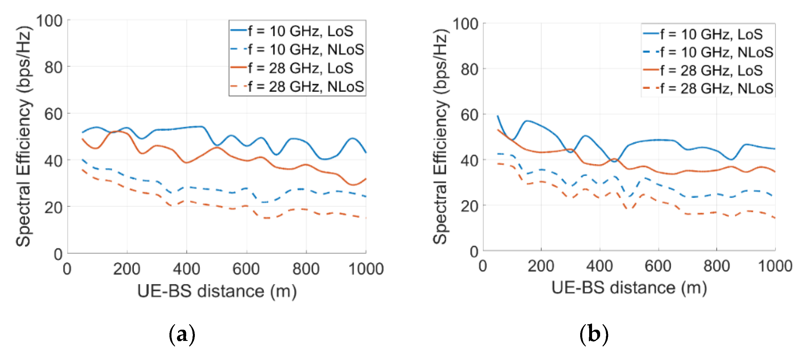
• A theoretical study is carried out in order to simulate a distributed massive MIMO system in the mmWave band. A deep analysis on the spectral efficiency is presented using the NYUSIM simulator;
• A field study is performed to emulate a distributed MIMO system in the mmWave band. A measurement campaign is performed to emulate several distributed MIMO scenarios above 30 GHz. A comparison with the power unbalance in the sub–6 GHz band is made in order to see the implementation viability of distributed MIMO scenarios for future mobile generations.

The study is organized as follows. Section 2 introduces the distributed MIMO model and the channel matrix that provides the spectral efficiency of the measured scenario. Section 3, Section 4 and Section 5 show the analysis of the D-MIMO scenarios in real deployments and simulations, and sub–6 GHz and mmWave bands. Finally, the main conclusions of the article are drawn in Section 6.

2. Distributed MIMO Model

The main goal to study the scenarios is the emulation of distributed MIMO systems by combining values from several communication channels acquired in different environments. Therefore, diverse channel matrices are combined in order to form a single matrix that symbolizes the D-MIMO channel matrix [6,19]. Each propagation environment has a certain number of transmitting (TX) and receiving (RX) antennas. TXs simulate a transmitting BS, where each BS is placed in a different location, emitting to a user equipment (UE) located in a fixed place and composed by several RXs. Mathematically, the combination of channel matrices can be depicted in Equation (1). A deep and detailed explanation on channel matrix models can be found on [20,21].

$$\mathit{H} = [{\mathit{H}}_1^T,{\mathit{H}}_2^T, \dots ,{\mathit{H}}_N^T]{ }^T,$$

(1)

N is the total number of MIMO systems that form the D-MIMO. ${\mathit{H}}_i$ is the channel matrix from a single MIMO whose dimension is ${\mathrm{L}}_i$ × R. ${\mathrm{L}}_i$ and R is the number of TX and RX in the BS and UE for the i-MIMO system, respectively. Finally, $\mathit{H}$ is the channel matrix of the D-MIMO with dimensions L × R, where L is computed as ${\displaystyle \sum }_{i=1}^N{\mathrm{L}}_i$.

It is essential to emphasize that each ${\mathit{H}}_i$, related to different MIMO systems, represents propagation channels that may differ from each other due to the unique conditions of each scenario. Therefore, the power received by the UE is expected to be different from different schemes. In this paper, a modulation of ${\mathit{H}}_i$ is introduced to emulate the unbalance power that might occur in a D-MIMO system. In order to perform this unbalance, ${\mathit{H}}_i$ is multiplied by a balance factor (Att) that emulates losses in the transmission due to obstacles in the propagation path or shadow fading.

$${\mathit{H}}_i^{Att}=At{t}_i·{\mathit{H}}_i ; At{t}_i\ge 0$$

(2)

By applying this balance factor to certain i-MIMO systems, the performance of D-MIMO systems can be analyzed when they suffer a strong power unbalance. The spectral efficiency of the system can be computed to determine the effect on the D-MIMO once the power balance is modified. This metric of the full communication channel is estimated using the following formulas [22]:

$${\mathit{H}}_{norm}\left(f_i\right)=\mathit{H}\left(f_i\right){ \left[\frac{1}{N_f}{\displaystyle \sum }_{i=1}^{N_f}{\left|\left|\mathit{H}\left(f_i\right)\right|\right|}^2\right]}^{-\frac{1}{2}},{ }^{ }$$

(3)

$$\eta \left(\mathrm{bps}/\mathrm{Hz}\right)=lo{g}_2\left|{\mathit{I}}_L+\frac{\mathrm{SIN}\mathrm{R}}{\mathrm{L}}\mathit{H}{\mathit{H}}^H\right|,{ }^{ }$$

(4)

where SINR is the signal-to-interference-plus-noise ratio rate, $\mathit{H}$ represents the channel matrix of the D-MIMO, $\mathit{I}$ is an identity matrix, and the superscript ${ }^{\left(H\right)}$ denotes the conjugate transpose operator. First of all, $\mathit{H}$ must be normalized (${\mathit{H}}_{norm}$) in order to take into account the frequency dependence of the communication channel in Equation (3) [23], where $N_f$ is the number of frequency samples. Note that the number of frequency samples $N_f$ must be chosen long enough so that no channel effect at a single frequency is unnoticed. The spectral efficiency in Equation (4) is calculated from the normalized channel frequency response ${\mathit{H}}_{norm}$. Throughout the article, additional modifications will be added to the channel frequency response shown in Equation (3) to demonstrate the importance of effects such as power unbalance in D-MIMO systems.

A visual example of the composition of a D-MIMO system is illustrated in the Figure 2. This example shows the composition of a D-MIMO throughout several measurements acquired in a semi-anechoic and semi-reverberation chamber. As previously stated, n–MIMO systems are deployed, where the UE/RX is located in a fixed position. However, the BS/TX position is changed in order to move and point to different locations inside the chamber. This provokes the diversity of the propagation channel which is finally reflected on the channel matrix $\mathit{H}$. Each one of the following sections details how the channel matrices ${\mathit{H}}_i$ were obtained.

3. Power Unbalance on Sub–6 Ghz D-MIMO Systems

This section presents the effect of the power unbalance for a D-MIMO system composed by multiple MIMO subsystems acquired in a reverberation chamber. The first part of the section briefly describes the acquisition process of the propagation channels. The second part shows and details the results of this power unbalance. From an analytical perspective, the relevance of this section lies in understanding how the spectral efficiency can be maximized while the power allocation is minimized at the same time.

3.1. Measurement Scenario

The first subset of measurements is taken in a reverberation chamber. These measurements are characterized by the rich scattering scenario generated inside the chamber. The reflection of the waves on the shielded walls creates several multipath components (MPCs) that reach the UE in different time instants, which increase the diversity of the scenario. Seven different scenarios are measured inside the reverberation chamber, where the BS has twelve transmitter antennas and UE has three receiver antennas. In order to generate diversity on the propagation channel, two mechanical stirrers are inserted inside the reverberation chamber. Since stirrers can adopt 50 different positions, together with 201 frequency points (250 kHz frequency spacing) from 1775 GHz to 1825 GHz, 10,050 channel propagation are measured for each TX-RX pair on each scenario. The main difference between the seven scenarios is found in the load of the reverberation chamber, which is changed by introducing several absorbers in different positions. A deep explanation of the measuring process can be found in [24,25].

Once the acquisition process is carried out, seven MIMO systems are achieved and saved on seven ${\mathit{H}}_i$. The full D-MIMO system is formed by the matrix $\mathit{H}= \left[{\mathit{H}}_1^T,{\mathit{H}}_2^T, \dots ,{\mathit{H}}_7^T\right]{ }^T$ whose dimensions are 84 TX × 3 RX.

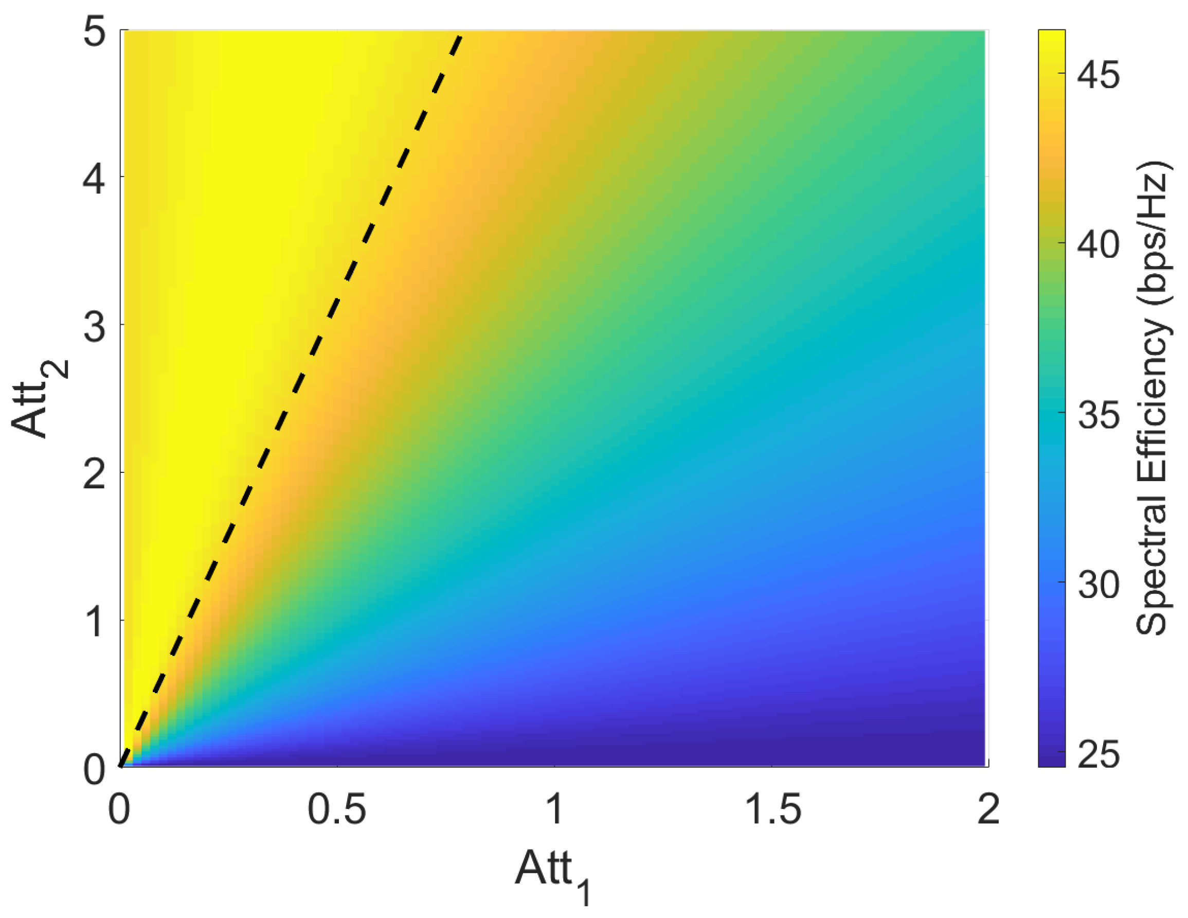
3.2. Power Balance Analysis

In order to analyze the effect of the power balance in a D-MIMO system, the balance of the measurements must be assessed. For that purpose,

Table 1. Normalized power balance (NPB) for the i-MIMO system.

	A (H1)	B (H2)	C (H3)	D (H4)	E (H5)	F (H6)	G (H7)
Power allocation	1	0.48	0.36	0.85	0.58	0.15	0.14

shows the normalized power balance (NPB) over the maximum value for the i-MIMO system. Since all scenarios are normalized, it can be seen that scenario A reaches the maximum power in the receivers. As stated in [22,23], this scenario lacks absorbers, so it is logical to expect maximum received power. The higher the number of absorbers, the lower the received power due to the absorption effect.

Once the power allocation is known, we can establish a D-MIMO system formed by the first transmitter of the scenarios from A to E and all three receivers from every scenario. This leads to a D-MIMO whose channel matrix H has the dimensions 5 TX × 3 RX. In this new H, the average value of the normalized power is 0.65. Scenarios A and B are modified by applying the balance factors $At{t}_1$ and $At{t}_2$ Equation (2) to the first two rows of H to see the effect of the power balance. Figure 3a shows the spectral efficiency of the D-MIMO when it is modulated with both balance factors simultaneously. As it can be seen, the higher the $At{t}_2$ value is, the higher the spectral efficiency obtained. Since $At{t}_2$ modulates ${\mathit{H}}_2$ ($\mathrm{NPB}=0.48$) and the average NPB for the full matrix H is 0.65, it is intended to obtain an $At{t}_2$ value as close as possible to 1. This fact provides an NPB in the ${\mathit{H}}_2$ row that is the closest to the average NPB. Observing the effect of $At{t}_1$, the spectral efficiency rises from 0.01 to 0.6, where it reaches a maximum. From that value, the metric tends to decrease. Since ${\mathit{H}}_1$ NPB is 1, the value of $At{t}_1$ that provides a NPB similar to the average NPB is 0.65. It is clearly observed that the maximum spectral efficiencies are reached for these values. In short, the D-MIMO is able to maximize its spectral efficiency when the i-MIMO systems tend to be balanced due to the balance factor inclusion.

In order to validate this reasoning, a second experiment was carried out. The first transmitter from the scenarios C, D, E, F and G were chosen. Therefore, a D-MIMO with channel matrix H (5 TX × 3 RX) was created. In this case, the average NPB is 0.42 and the balance factors $At{t}_3$ and $At{t}_4$ are applied to the scenarios C (${\mathit{H}}_3$) and D (${\mathit{H}}_4$), respectively. Figure 3b presents the spectral efficiency when both balance factors are included. First, the NPB in scenario C is 0.36. Therefore, larger values of $At{t}_3$ obtain a NPB closer to the average NPB of the D-MIMO. Consequently, the spectral efficiency increases as $At{t}_3$ increases. Based on the modulation of scenario D ($At{t}_4$), the NPB is 0.85. In order to maximize the spectral efficiency, the NPB must tend to values around the average NPB. This is obtained for values of $At{t}_4$ around 0.5. Note that $At{t}_4$ values above 0.5 do not increase the spectral efficiency even when it implies increasing the transmission power of scenario C. This fact is due to the power unbalance when $At{t}_4$ is too high.

To conclude this section, it was proven that the spectral efficiency of a D-MIMO system is directly proportional to the power balance. Therefore, the received power variance between the TX-RX pair should be reduced in order to provide satisfactory UE services.

4. Correlation and Los on Emulated D-MIMO Systems above 6 Ghz

4.1. Emulation Scenario

In this section, an analysis on the TX correlation and the effect of the line-of-sight (LoS) in D-MIMO systems is performed. For that purpose, several measurements of the propagation channel are simulated in NYUSIM [26]. NYUSIM is a mmWave simulator that has a wide variety of configuration parameters for the simulated environment. In particular, it allows to simulate scenarios for a wide frequency range and several propagation models. In this study, simulations from 10 GHz to 78 GHz are carried out for two environment models: urban macrocell (UMa) and urban microcell (UMi). Several channel matrices H were simulated for a wide range of configuration parameters.

Table 2. NYUSIM simulation parameters.

Simulation Parameters
Frequency	10 GHz, 28 GHz, 40 GHz and 78 GHz
Bandwidth	800 MHz
Frequency samples	1601 (500 kHz frequency spacing)
Propagation environment	Urban macrocell (UMa) and urban microcell (UMi)
Visibility	Line-of-sight (LoS) and non-line-of-sight (NLoS)
UE-BS distance	50 to 1000 m
TX antennas in the BS	200 antennas (Lineal array)
RX antennas in the UE	20 antennas (Lineal array)
TX antenna separation	λ/10, λ/2 and λ
RX antenna separation	λ/10, λ/2 and λ
EIRP	30 dBm
Iterations	10

shows the choice of simulation parameters in detail. Note that each simulation was iterated ten times in order to avoid outliers in the channel matrices H. The chosen distances, antenna spacing, and frequencies ensure the UE far-field condition for all simulations shown in this section.

4.2. Correlation and LoS Analysis

The first test consists of studying the TX/RX antenna spacing in the BS/UE to determine its effect on spectral efficiency. For that purpose, a D-MIMO system with 50 TX and 10 RX was created. The D-MIMO is formed by 3 BS which are 100 m, 120 m, and 140 m away from the receiver. The relative distance between BSs is set to be the largest BS-UE distance (140 m). On each BS the transmission is made with 17 TX, 17 TX, and 16 TX, respectively. The simulations are made for two environments (UMa and UMi) and three frequencies (28 GHz, 40 GHz, and 78 GHz). Since the goal is to study the TX/RX antenna spacing effect, three distances are considered for the TX/RX spacing: λ/10, λ/2, and λ. For the sake of clarity, the spacing is set to the same value on both sides of the communication. Theoretically, the closer the antennas are to each other, the lower the benefit from spatial diversity is due to the higher correlation between channels. Figure 4a,b show the results for this test. We define Θ as the difference between the Shannon theoretical limit and the spectral efficiency simulated. The Shannon theoretical limit establishes the spectral efficiency for completely decorrelated channels. Therefore, the Shannon limit cannot be exceeded and Θ provides an idea of how far the scenario is from the theoretical limit. Looking at both scenarios, UMa (Figure 4a) and UMi (Figure 4b), the UMa scenario tends to obtain similar results for all frequencies, while the UMi scenario shows differences up to 3 bps/Hz due to the frequency band. However, the main effect is induced by the TX/RX spacing. The farther apart the TX and RX are spaced in the ULA, the closer the theoretical limit of spectral efficiency is. In this case, the propagation channel looks different for the receivers and the propagation channels become independent from each other. Therefore, we can take advantage of the spatial multiplexing and the spectral efficiency to be closer to the Shannon limit. It is remarkable that curves between λ/10 and λ/2 are more separated than curves between λ/2 and λ. This fact shows that a λ/10 spacing significantly affects the channel due to the high correlation. However, spacing values above λ/2 are enough decorrelated to take advantage of the channel diversity. In absolute terms, the improvement from λ/10 to λ/2 is 13 bps/Hz (UMa) and 12 bps/Hz (UMi). Nevertheless, the improvement from λ/2 to λ is only 2 bps/Hz (UMa) and 5 bps/Hz (UMi). In conclusion, a wider spacing between BS antennas allows an increase in spectral efficiency for the user by decreasing the antenna correlation and increasing the independence of the communication channels.

The second test studies the influence of LoS and NLoS on the communication channels of a D-MIMO system. A D-MIMO formed by 50 TX and 10 RX is analyzed, where 2 BS are considered (25 TX per BS). Both BS are moved simultaneously from 50 to 1000 m away from the UE. The relative distance between BSs is set to be the BS-UE distance. According to the previous test, the antenna spacing is set to λ/2. Two environments were tested (UMa and UMi) and two frequencies were considered (10 GHz and 28 GHz). Figure 5a,b show the spectral efficiency of both frequencies and visibility conditions in function of the distance between the UE and both BSs for the UMa and UMi scenario respectively. For the UMa and UMi environment (LoS and NLOS cases), the spectral efficiency slightly decreases over distance due to attenuation in the propagation path. This decrease is not linear. Due to fading effects, there are distances where a constructive contribution of the multipath environment implies an increase in the efficiency. Likewise, at other distances, a destructive contribution from the multipath environment decreases the efficiency. Note that the 28 GHz channel also has lower efficiency than the 10 GHz channel due to higher attenuation. However, besides all effects mentioned, the main one is the LoS/NLoS condition. For both environments, the spectral efficiency is increased by approximately 25% when the propagation path includes the Line-of-Sight. In conclusion, the network deployment for massive D-MIMO systems should ensure a spacing antenna above λ/2 and should provide the UE with LoS to maximize the spectral efficiency of the communications.

5. D-MIMO System on a Semi-Anechoic and Semi-Reverberation Chamber in the mmWave Band

5.1. Measurement Scenario

This last section is focused on the analysis of a D-MIMO system in the mmWave band acquired in a controlled scenario, such as a semi-anechoic and semi-reverberation chamber. For that purpose, two distinct scenarios are taken into account. On the one hand, the semi-anechoic part is commonly used for the characterization of radiating elements due to the absorption of any reflection in the scenario. In this case, it is used as a communication channel where the lack of reflections decreases the diversity of the scenario. Only one direct beam reaches the receiver through the LoS. Therefore, it is expected to notice a very high correlation between channel measurements. On the other hand, the semi-reverberation part implies a rich scattering environment since the metallic walls generate several propagation paths for the electromagnetic waves. In this case, any movement on the BS/UE generates a totally different propagation path, which makes the correlation between channels low. A complete and detailed description of the chamber is available in [27].

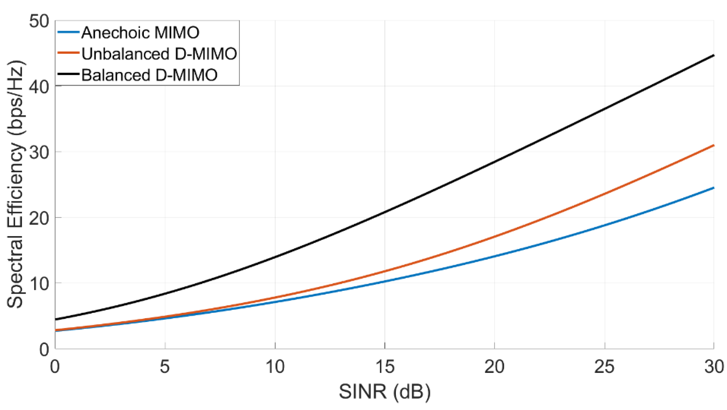
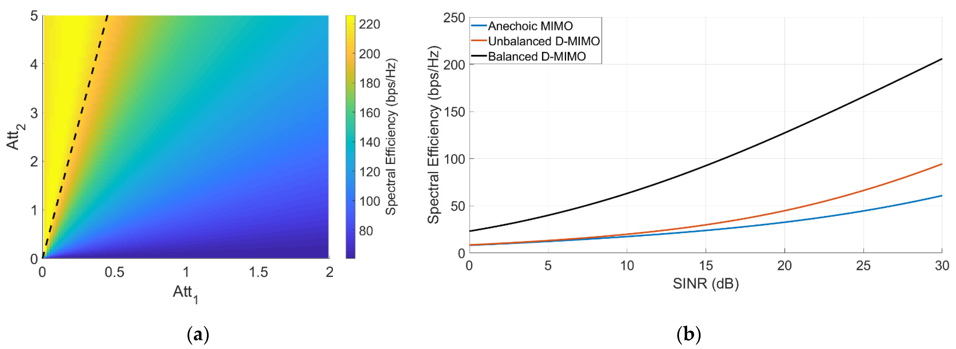
5.2. Anechoic and Reverberation Channel Analysis

Once the two types of propagation channels are known, two MIMO systems are acquired. The first one has a BS with 11 TX pointing the UE in the semi-anechoic part. The transmitters are arranged at 90° amplitude in the azimuth angle, with an angle separation between consecutive transmitters of 9°. The UE is composed by 5 RX in a 20 cm lineal array, where the separation between consecutive RX is 5 cm. The frequency range of the measurement goes from 40 GHz to 50 GHz for 101 frequency samples (100 MHz frequency spacing) and the distance on the LoS is 150 cm. The second MIMO measured is similar to the first one. The main difference lies on the BS pointing angle. In this case, the BS points directly to the metallic wall in the semi-reverberation part, which makes a NLoS scenario where the signal reaches the RX through several reflections. In this case, the shortest path from the TX to the RX is 720 cm.

Due to the peculiarities of the scenarios, several conclusions can be drawn. The anechoic channels are expected to achieve lower attenuations due to the proximity between the pair TX/RX. However, the correlation between channels will be high due to the low spatial diversity of the scenario. On other hand, the reverberation channels are expected to obtain higher attenuations due to the TX-RX distance. Nevertheless, the channels tend to be independents.

Once the previous facts were known, we created a D-MIMO system formed by both MIMO systems. A matrix channel $\mathit{H} = \left[{\mathit{H}}_1^T,{\mathit{H}}_2^T\right]{ }^T$ with dimensions 22 TX × 5 RX for 101 frequency samples was obtained. The normalized power balance for the submatrix ${\mathit{H}}_1$ and ${\mathit{H}}_2$ is 1 and 0.158, respectively. As previously stated, the anechoic channels achieve the maximum power, and the reverberation channels are attenuated in a factor 6.325 in average. Without the application of a normalization factor, reverberation channels will be masked by the anechoic channels. Therefore, as shown in Section 3, $At{t}_1$ and $At{t}_2$ factors multiply the anechoic and reverberation channels in order to modulate the D-MIMO balance power. Figure 6 shows a parametric sweep of both factors for the spectral efficiency. $At{t}_1$ moves in the range from 0 to 2 and $At{t}_2$ in the range from 0 to 5. Moreover, a black line with slope 6.325 is shown. This line represents those operating points where the D-MIMO is balanced in terms of power. On the right side of this line, the D-MIMO system is dominated by anechoic channels, while the reverberation channels prevail in the left side. The higher the prevalence of the anechoic channels, the lower the spectral efficiency due to the high correlation between these channels. As we approach the equilibrium line, the presence of the significantly less correlated reverberation channels becomes higher, which increases the efficiency. In the balanced region, the efficiency is maximized around 45 bps/Hz. On the left side, the values remain around the maximum because the reverberation channels are the predominant ones over the anechoic channels.

Finally, to further explore this scenario, three key operating points were studied in terms of SINR. Figure 7 illustrates the spectral efficiency of the MIMO subsystem formed by the anechoic channels, the unbalanced D-MIMO and the balanced D-MIMO. The first curve takes into account only the ${\mathit{H}}_1$ channel matrix. For 30 dB SINR, it reaches a spectral efficiency of 24.5 bps/Hz. This operating point is shown in Figure 6 for $At{t}_1=1$ and $At{t}_2=0$. If we include the reverberation channels, the unbalanced D-MIMO is formed. In this case, diversity is added to the scenario, although reverberation channels are masked due to unbalancing. The effect can be seen in the second curve, where the spectral efficiency is slightly improved. This operating point corresponds to $At{t}_1=1$ and $At{t}_2=1$, where the spectral efficiency is 30.9 bps/Hz in Figure 6. Finally, the channel power balance can improve further the scenario. This effect is shown in the third curve, where the spectral efficiency is significantly improved ($At{t}_1=0.158$ and $At{t}_2=1$). Due to this fact, values up to 45 bps/Hz are achieved. This means an improvement of 45.6% compared with the unbalanced case and 83.7% compared with the anechoic subsystem.

Once the previous case was studied, a second set of measurements was acquired. On the one hand, 33 TX points the UE in the semi-anechoic chamber. As in previous case, TXs are arranged at a 90° amplitude in the azimuth angle with a separation of 9° (11 locations). However, we added 11 TX 5 cm on the left and 11 TX 5 cm on the right to form a ULA. Each position includes 11 TX that varies in the azimuth angle, for a total of 33 TX. On the other hand, the UE is composed of 25 RX in a 20 cm uniform rectangular array (URA), where the separation between the consecutive RX is 5 cm in both axes. The second MIMO is similar to the first one, but pointing the semi-reverberation chamber. The distances and frequency ranges are the same as in the previous example.

After the acquisition, the D-MIMO channel matrix is formed by combining both MIMO system, whose size is 66 TX × 25 RX. The normalized power balance for the anechoic MIMO and reverberation MIMO is 1 and 0.091, respectively. This means the reverberation MIMO is even more unbalanced than in Figure 6. Specifically, reverberation channels are attenuated in an 11.042 factor compared with the anechoic channels. Figure 8A presents a sweep parameter for $At{t}_1$ and $At{t}_2$ factors, where we can extract similar conclusions as in Figure 6. Note that the black line which indicates the balance power equilibrium is shifted to the left. This is due to the larger unbalance from the reverberation chamber. The slope of this equilibrium point is 11.042. In the balance region, the spectral efficiency is maximized around 205 bps/Hz. Figure 8B shows the operation points previously illustrated in Figure 7. When the number of propagation channels increases and the power distribution is balanced, the spectral efficiency is also expected to increase. For a 30 dB SINR, the anechoic MIMO obtains 60.7 bps/Hz, the unbalanced D-MIMO gets 94.3 bps/Hz and the balance D-MIMO achieves 205.8 bps/Hz. In relative terms, the balanced D-MIMO system has an improvement of 118.3% compared with the unbalanced case and 238.9% compared with the anechoic subsystem. These results show how critical a proper assignation of the power resources is for massive D-MIMO systems.

The analysis made in this section shows that decorrelation of channels in a D-MIMO, as well as channel power balance, imply the improvement of propagation channel conditions, ensuring both conditions induce optimal physical channel performance. Furthermore, by comparing both D-MIMOs, it was shown that the higher the number of propagation channels are, the more noticeable this improvement is.

6. Conclusions

In the current work, an analysis of the performance of D-MIMO systems under different conditions was carried out. Several MIMO scenarios have been proposed. On the frequency side, several bands were studied, including the sub–6 GHz and the mmWave band. On the scenario side, both simulated and real measurements were analyzed for a wide variety of environments. Rural and urban scenarios were emulated, and channels from anechoic and reverberation chambers were acquired.

The analysis of all these measurements was focused on the balance power and the correlation between propagation channels for distributed MIMO systems. These systems are expected to be fundamental in the future deployment of mobile networks due to the large number of antennas which allows high spectral efficiencies. In this study, it was found that D-MIMO provides high data rates compared with common MIMO systems. However, it is fundamental to perform an accurate deployment analysis in order to find decorrelated and balanced propagation channels in terms of power. Throughout the study, we observed how the combination of both properties takes full advantage of the benefits of the propagation channel, significantly increasing the spectral efficiency on the physical layer of the communication channels. The network operation following design criteria such as those seen in this study is fundamental for the multi-connectivity expected in D-MIMO systems. An optimal choice of such criteria showed network performances of 45.6% (22 TX × 5 RX D-MIMO) and 118.3% (66 TX × 25 RX D-MIMO) better than non-optimal cases in terms of spectral efficiency for similar D-MIMO systems but with different power allocation criteria.

References

1. Ericsson. Ericsson Mobility Report June 2021. 2021. Available online: https://www.ericsson.com/4a03c2/assets/local/mobility-report/documents/2021/june-2021-ericsson-mobility-report.pdf (accessed on 29 September 2021).
2. Cisco. Cisco Annual Internet Report (2018–2023). 2020. Available online: https://www.cisco.com/c/en/us/solutions/collateral/executiveperspectives/annual-internet-report/white-paper-c11-741490.html (accessed on 29 September 2021).
3. Han, B.; Liu, Y.; Qian, F. ViVo: Visibility-aware mobile volumetric video streaming. In Proceedings of the 26th Annual International Conference on Mobile Computing and Networking, London, UK, 21–25 September 2020; Association for Computing Machinery: New York, NY, USA, 2020; pp. 1–13. [Google Scholar]
4. Ramirez-Arroyo, A.; Zapata-Cano, P.H.; Palomares-Caballero, A.; Carmona-Murillo, J.; Luna-Valero, F.; Valenzuela-Valdes, J.F. Multilayer Network Optimization for 5G & 6G. IEEE Access 2020, 8, 204295–204308. [Google Scholar]
5. Albreem, M.A.; Juntti, M.; Shahabuddin, S. Massive MIMO Detection Techniques: A Survey. IEEE Commun. Surv. Tutor. 2019, 21, 3109–3132. [Google Scholar] [CrossRef] [Green Version]
6. MacCartney, G.R.; Rappaport, T.S. Millimeter-Wave Base Station Diversity for 5G Coordinated Multipoint (CoMP) Applications. IEEE Trans. Wirel. Commun. 2019, 18, 3395–3410. [Google Scholar] [CrossRef]
7. Jungnickel, V.; Manolakis, K.; Zirwas, W.; Panzner, B.; Braun, V.; Lossow, M.; Sternad, M.; Apelfröjd, R.; Svensson, T. The role of small cells, coordinated multipoint, and massive MIMO in 5G. IEEE Commun. Mag. 2014, 52, 44–51. [Google Scholar] [CrossRef]
8. Zhang, J.; Ji, Y.; Jia, S.; Li, H.; Yu, X.; Wang, X. Reconfigurable Optical Mobile Fronthaul Networks for Coordinated Multipoint Transmission and Reception in 5G. J. Opt. Commun. Netw. 2017, 9, 489–497. [Google Scholar] [CrossRef]
9. Yu, Y.-J.; Hsieh, T.-Y.; Pang, A.-C. Millimeter-Wave Backhaul Traffic Minimization for CoMP Over 5G Cellular Networks. IEEE Trans. Veh. Technol. 2019, 68, 4003–4015. [Google Scholar] [CrossRef]
10. Bassoy, S.; Farooq, H.; Imran, M.A.; Imran, A. Coordinated Multi-Point Clustering Schemes: A Survey. IEEE Commun. Surv. Tutor. 2017, 19, 743–764. [Google Scholar] [CrossRef]
11. Bassoy, S.; Imran, M.A.; Yang, S.; Tafazolli, R. A Load-Aware Clustering Model for Coordinated Transmission in Future Wireless Networks. IEEE Access 2019, 7, 92693–92708. [Google Scholar] [CrossRef]
12. Chen, S.; Zhao, T.; Chen, H.-H.; Lu, Z.; Meng, W. Performance Analysis of Downlink Coordinated Multipoint Joint Transmission in Ultra-Dense Networks. IEEE Netw. 2017, 31, 106–114. [Google Scholar] [CrossRef]
13. Schwarz, S.; Rupp, M. Exploring Coordinated Multipoint Beamforming Strategies for 5G Cellular. IEEE Access 2014, 2, 930–946. [Google Scholar] [CrossRef]
14. Marotta, A.; Cassioli, D.; Antonelli, C.; Kondepu, K.; Valcarenghi, L. Network Solutions for CoMP Coordinated Scheduling. IEEE Access 2019, 7, 176624–176633. [Google Scholar] [CrossRef]
15. Li, L.; Yang, C.; Mkiramweni, M.E.; Pang, L. Intelligent Scheduling and Power Control for Multimedia Transmission in 5G CoMP Systems: A Dynamic Bargaining Game. IEEE J. Sel. Areas Commun. 2019, 37, 1622–1631. [Google Scholar] [CrossRef]
16. Georgakopoulos, P.; Akhtar, T.; Politis, I.; Tselios, C.; Markakis, E.; Kotsopoulos, S. Coordination Multipoint Enabled Small Cells for Coalition-Game-Based Radio Resource Management. IEEE Netw. 2019, 33, 63–69. [Google Scholar] [CrossRef]
17. Mismar, F.B.; Evans, B.L. Deep Learning in Downlink Coordinated Multipoint in New Radio Heterogeneous Networks. IEEE Wirel. Commun. Lett. 2019, 8, 1040–1043. [Google Scholar] [CrossRef] [Green Version]
18. Song, G.; Wang, W.; Chen, D.; Jiang, T. KPI/KQI-Driven Coordinated Multipoint in 5G: Measurements, Field Trials, and Technical Solutions. IEEE Wirel. Commun. 2018, 25, 23–29. [Google Scholar] [CrossRef]
19. Park, S.; Alkhateeb, A.; Heath, W.R., Jr. Dynamic Subarrays for Hybrid Precoding in Wideband mmWave MIMO Systems. IEEE Trans. Wirel. Commun. 2017, 16, 2907–2920. [Google Scholar] [CrossRef]
20. Li, J.; Wang, D.; Zhu, P.; Wang, J.; You, X. Downlink Spectral Efficiency of Distributed Massive MIMO Systems with Linear Beamforming Under Pilot Contamination. IEEE Trans. Veh. Technol. 2018, 67, 1130–1145. [Google Scholar] [CrossRef] [Green Version]
21. Lv, Q.; Li, J.; Zhu, P.; You, X. Spectral Efficiency Analysis for Bidirectional Dynamic Network with Massive MIMO Under Imperfect CSI. IEEE Access 2018, 6, 43660–43671. [Google Scholar] [CrossRef]
22. Marzetta, T.L.; Larsson, E.G.; Yang, H.; Ngo, H.Q. Fundamentals of Massive MIMO; Cambridge University Press: Cambridge, UK, 2018. [Google Scholar]
23. Loyka, S.; Levin, G. On physically-based normalization of MIMO channel matrices. IEEE Trans. Wirel. Commun. 2009, 8, 1107–1112. [Google Scholar] [CrossRef]
24. Valenzuela-Valdes, J.; Martinez-Gonzalez, A.; Sanchez-Hernandez, D. Emulation of MIMO Nonisotropic Fading Environments with Reverberation Chambers. IEEE Antennas Wirel. Propag. Lett. 2008, 7, 325–328. [Google Scholar] [CrossRef] [Green Version]
25. Valenzuela-Valdes, J.; Martinez-Gonzalez, A.; Sanchez-Hernandez, D. Diversity Gain and MIMO Capacity for Nonisotropic Environments Using a Reverberation Chamber. IEEE Antennas Wirel. Propag. Lett. 2009, 8, 112–115. [Google Scholar] [CrossRef] [Green Version]
26. Ju, S.; Kanhere, O.; Xing, Y.; Rappaport, T.S. A Millimeter-Wave Channel Simulator NYUSIM with Spatial Consistency and Human Blockage. In Proceedings of the 2019 IEEE Global Communications Conference (GLOBECOM), Waikoloa, HI, USA, 9–13 December 2019; pp. 1–6. [Google Scholar]
27. Ramírez-Arroyo, A.; Alex-Amor, A.; García-García, C.; Palomares-Caballero, Á.; Padilla, P.; Valenzuela-Valdés, J.F. Time-Gating Technique for Recreating Complex Scenarios in 5G Systems. IEEE Access 2020, 8, 183583–183595. [Google Scholar] [CrossRef]
Figure 1. Evolution roadmap of the communication standards and major technological challenges for future mobile communications.
Applsci 11 10926 g001
Figure 2. Scheme of a D-MIMO consisting of a set of MIMO subsystems acquired in a semi-anechoic and semi-reverberation chamber.
Applsci 11 10926 g002
Figure 3. Spectral efficiency of a D-MIMO when the power balance is modulated with two balance factors. SINR is fixed to 15 dB. The i-MIMO systems that form the D-MIMO are the scenarios (a) A ( A t t 1 ), B ( A t t 2 ), C, D, E, and (b) C ( A t t 3 ), D ( A t t 4 ), E, F, G.
Applsci 11 10926 g003
Figure 4. Distance to the spectral efficiency theoretical limit for three frequencies (28 GHz, 40 GHz and 78 GHz) and three TX/RX antenna spacing (λ/10, λ/2 and λ) for several SINR values in a D-MIMO (50 × 10). (a) UMa scenario and (b) UMi scenario.
Applsci 11 10926 g004
Figure 5. Spectral efficiency of a D-MIMO (50 × 10) system for two frequencies (10 GHz and 28 GHz) and LoS and NLoS visibility conditions. SINR is fixed to 15 dB. (a) UMa scenario and (b) UMi scenario.
Applsci 11 10926 g005
Figure 6. Spectral efficiency for a parametric sweep of A t t 1 and A t t 2 . The black line stands for the region where both MIMO subsystems are balanced in terms of power. The SINR is fixed to 30 dB and the values are averaged over the 101 frequency samples.
Applsci 11 10926 g006
Figure 7. Spectral efficiency for the anechoic MIMO (blue line), unbalanced D-MIMO (red line) and balanced MIMO (black line). For each value of SINR, the spectral efficiency is averaged over the 101 frequency samples.
Applsci 11 10926 g007
Figure 8. (a) Spectral efficiency (D-MIMO 66 × 25) for a parametric sweep of A t t 1 and A t t 2 and (b) spectral efficiency for the anechoic MIMO (blue line), unbalanced D-MIMO (red line) and balanced MIMO (black line).
Applsci 11 10926 g008