Abstract
This paper derives an original finite element for the static bending analysis of a transversely cracked uniform beam resting on a two-parametric elastic foundation. In the simplified computational model based on the Euler–Bernoulli theory of small displacements, the crack is represented by a linear rotational spring connecting two elastic members. The derivations of approximate transverse displacement functions, stiffness matrix coefficients, and the load vector for a linearly distributed load along the entire beam element are based on novel cubic polynomial interpolation functions, including the second soil parameter. Moreover, all derived expressions are obtained in closed forms, which allow easy implementation in existing finite element software. Two numerical examples are presented in order to substantiate the discussed approach. They cover both possible analytical solution forms that may occur (depending on the problem parameters) from the same governing differential equation of the considered problem. Therefore, several response parameters are studied for each example (with additional emphasis on their convergence) and compared with the corresponding analytical solution, thus proving the quality of the obtained finite element.
1. Introduction
The occurrence of cracks in the structure is considered to be one of the most unfavorable effects, since their presence may lead to the collapse in extreme cases. It is well known that the stress and strain in structural elements such as beams or columns increase significantly at the location of cracking. This leads not only to a reduction in stiffness but also to a change in the response pattern, the magnitude of which depends mainly on the location and depth of the crack. In the static analysis of structures, cracked beams are usually considered as a one-dimensional continuum with local stiffness reduction, since such models allow simpler and faster but still reliable response calculations. When the stress distribution near the crack is not of interest, a simplified computational model in which two adjacent elastic non-cracked segments are connected at the crack location by a corresponding (rotational and/or translational) point spring is particularly suitable. In addition, such a model allows an effective representation of the depth and location of the crack. In the pure bending of slender Euler–Bernoulli beams, the presence of cracks mainly affects the bending stiffness, so the point spring can be justifiably represented by the rotational contribution only [1].
This rotational spring can also be effectively implemented into the computational model of cracked beams on an elastic soil, which has already been confirmed by many studies in the field of structural mechanics [2,3,4,5]. Most studies idealize soils by the classical one-parameter Winkler model [6], in which the real compressive strength of soils is represented by individual and unconnected vertical compression springs. Furthermore, a recent study introduces a new exact finite element for static analysis, which contains accurate interpolation functions obtained from the differential equation solutions of a transversely cracked beam on Winkler soil [7].
In addition to Winkler’s compressive contribution, the mechanical strength of the actual soil includes the shear contribution of deformations. Therefore, an additional parameter is included for a more detailed description of the soil behavior that also takes into account the shear interaction between Winkler springs. By implementing the shear interaction between the springs as a supplementary parameter, deformations and displacements of the soil can be calculated even outside the loaded area, allowing the behavior of the soil to be described much more realistically compared to single parameter formulation. In the two-parametric model, the actual shear interaction between Winkler springs is considered by introducing a second soil parameter. Several two-parametric models were presented by many authors based on different physical assumptions. The shear interaction between springs was first represented by an elastic membrane layer (Filonenko–Borodich model), then by an elastic beam (Heteny model), and finally by an elastic shear layer (Pasternak model), which is the most natural representation of the shear contribution of the soil. Generally, all these models mathematically share the same governing differential equation [8].
Although the analytical approach to solving differential equations provides exact solutions, the finite element method is primarily used in modern static analysis of beams on elastic soil, which is mostly due to the mathematical complexity of the analytical solution of differential equations. The accuracy and speed of convergence of the results depend not only on the applied mesh of elements but also on the quality of the applied finite elements.
Therefore, the novelty of this article is a closed-form original finite element for static bending analysis of the uniform Euler–Bernoulli transversely cracked beam on two-parametric soil. All expressions were derived from newly derived cubic polynomial interpolation functions in which the second soil parameter was included directly.
2. Basic Assumptions and General Analytical Formulation
The study considers a straight uniform slender transversely cracked beam with a rectangular constant cross-section resting on a deformable (elastic) soil. Since the bending of a beam with a transverse crack in the vertical plane is analyzed, the Opening Mode (Mode I) is considered. This mode is reflected in the different slopes to the left and right of the crack. Therefore, the discrete crack is introduced into the mathematical model through Okamura’s approach [1]. Although each transverse crack is geometrically defined by the location L1 and depth d, it is modeled by a rotational spring in the considered solution, as shown in Figure 1.
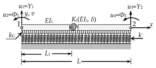
Figure 1.
Mathematical model of a beam with crack on the two-parametric soil.
Okamura et al. defined the genuine spring stiffness Kr as:
This original spring stiffness definition takes into account the non-cracked bending stiffness of the beam EIz, the height of the non-cracked part of the cross-section h, Poisson’s ratio ν, the relative crack depth δ′ = d/h, and the compliance function F(δ′).
In addition to Okamura, several other authors have provided their definitions, which implement the same general definition form of Kr but with different compliance functions [9,10,11,12].
The derivations represent the soil (defined as isotropic, homogeneous, and linear material) as a two-parameter elastic medium. The governing equilibrium differential equation for the non-cracked beams takes the form [8]:
where v(x)—transverse displacement function; k—coefficient of proportionality derived from the genuine Winkler’s soil coefficient; kG—the second soil parameter; q(x)—continuous transverse load. When searching for the analytical solution, two auxiliary parameters (λ1 and λ2) are implemented, which can be altogether presented by:
If the value of kG equals zero, both expressions reduce into a single parameter, which is already known from the genuine Winkler model solution. However, when solving the governing differential equation of a two-parametric soil, there is an important difference compared to the equivalent Winkler soil differential equation where a single analytical solution is obtained regardless of the combination of the beam and soil coefficients. Namely, for some combinations of two-parametric soil mechanical parameters, the second parameter becomes an imaginary value. Consequently, there are two different forms of analytical solutions () of Equation (3) [13]. For the case of kG2 < 4·EIz·k, the solution of Equation (3) obtains the following form:
while for the case of kG2 ≥ 4·EIz·k, the solution is:
where ai (i = 1, 2, 3, 4) are integration constants.
3. Derivation of a New Finite Element
For the purposes of numerical bending analyses, a new finite element of a singly transversely cracked Euler–Bernoulli beam on an elastic two-parametric soil is derived in this section. All the assumptions (regarding the beam, the crack, and the subgrade) considered in the analytical formulation of the problem are also applied in the derivation of the finite element. The equivalent rotational spring connecting two adjacent segments is located at a distance L1 from the left edge (node 1). The presented finite element of length L has two nodes and a total of four standard degrees of freedom. These are the (upwards positive) transverse displacement Y1 and the (anticlockwise) rotation Φ1 in the left node 1, as well as the (upwards positive) transverse displacement Y2 and the (anticlockwise) rotation Φ2 in the right node 2, as shown in Figure 1.
3.1. Derivation of Interpolation Functions of the Cracked Beam on the Two-Parametric Medium
As in many similar derivations, and primarily in order to universally cover both possible cases related to the parameter λ2 by a unique finite element solution, the complete cubic polynomials are implemented as interpolation functions. Due to the presence of the crack, which divides the beam into two elastic parts, separate interpolation functions are required for the parts to the left and the right. Since the finite element has four standard degrees of freedom, this consequently requires eight constants to be determined. They are determined from four boundary as well as four continuity conditions (the equality of displacements, the condition for the discrete slope increase, the equality of bending moments, and the equality of shear forces) at the crack location where the influence of the crack is introduced as a slope discontinuity. Although the general description of the continuity conditions is identical to the similar Winkler soil, there is an important computational difference since the second soil parameter kG is now directly introduced into the derivation of interpolation functions through the condition of shear forces equilibrium, i.e.,
Thus, the following functions of transverse displacements are obtained for the sections to the left and right of the crack, as shown in Equations (8) and (9):
with the following interpolation functions (x) and (x) (i = 1, 2, 3, 4), as shown in Equations (10) and (11):
The coefficients Ai,j (i, j = 1, 2, 3, 4) from interpolation functions of the first elastic part can be expressed by implementing the Dirac δ function as:
with the three following abbreviations:
Considering all four conditions of continuity at the crack location, the coefficients of the interpolation functions of the second part can be written by the coefficients of the first part as follows:
It should be noted that for the non-cracked case (δ′ = 0), these functions reduce into standard polynomial interpolation functions for the non-cracked case.
3.2. Derivation of Matrices of the Cracked Beam on the Two-Parametric Medium
The entire deformation energy U can be expressed as a sum of the contributions from the beam (from both elastic parts as well as the spring) and the soil:
where the first two terms belong to the strain energy in the beam elastic non-cracked parts, the third term corresponds to the contribution of the crack through the rotational spring energy, the fourth and the fifth term represent the strain energy of the Winkler soil, and the last two terms stand for the second soil parameter contribution, respectively.
Since the interpolation functions are known, transverse displacements from Equations (8) and (9) can be implemented in Equation (20). Furthermore, the complete 4 × 4 stiffness matrix [k] of a cracked beam finite-element on two-parametric soil can be thus expressed as:
where {N1} and {N2} represent the interpolation function vectors of the first and the second elastic part, respectively.
Thus, Equation (21) clearly shows the separate contributions of all the beam and soil parameters of the stiffness matrix. Every element of each separate contribution of kb,ij, ks1,ij, and ks2,ij (i, j = 1, 2, 3, 4) of stiffness matrix [k] is presented in a closed form expression as:
Each element kij (I, j = 1, 2, 3, 4) of the entire stiffness matrix can be further straightforwardly presented as a sum of all three separate contributions:
Moreover, Equations (22)–(25) may be generally presented in a more convenient form with a single expression:
where the coefficients ξ1 and ξ2 define the matrix being calculated. For ξ1 = ξ2 = i (with i = 1, 2, 3), Equation (26) reduces into the beam stiffness matrix element kb,ij, the first soil matrix element ks1,ij, and the second soil matrix element ks2,ij, as shown in Equations (22)–(24), respectively. Furthermore, each term of the complete stiffness matrix, Equation (25), can be directly obtained by taking ξ1 = 1 and ξ2 = 4.
3.3. Derivation of Load Vector Due to a Continuous Load q(x) over the Whole Element
To complete the finite element solution for the cases where continuous loads are considered, the load vector is also required. This vector consists of nodal forces and moments that replace the actual distributed load q(x) (upwards positive) over the finite element. These terms are derived from the conditions of work-equivalency where the work W is calculated due to distributed transverse load q(x) as:
The equation is further expressed in terms of vectors of unknown nodal displacements (degrees of freedom) {u}:
where the complete expressions in external curved brackets represent the substitutive load vector {Fq(x)} = {F1, F2, F3, F4}T. If qL and qR represent values of the load at the starting and ending node, respectively, the four load vector coefficients Fi (i = 1, 2, 3, 4) for a linearly distributed load (upward positive) obtain the form:
This newly presented finite element solution was entitled cracked beam on 2 parametric soil Finite Element (cb2psFE).
3.4. Computation of Nodal Shear Forces and Bending Moments
The corresponding element equilibrium equation in FEM formulation is:
where {Q} is the vector of secondary variables. Assembling the stiffness matrix and the load vector of the structure allows us to first obtain the nodal displacements and rotations for all the finite elements. Shear forces and bending moments at both nodes of the finite element are further calculated from the vector of secondary variables {Q}, as obtained from Equation (30):
consisting of the discrete values of shear forces (Vy1 and Vy2) and bending moments (Mz1 and Mz2).
3.5. Calculation of Bending Moment Functions
Two approaches can generally be applied to obtain the bending moment distribution functions, differing in the implemented method as well as in the degree of the resulting polynomials.
The well-known mechanical differential relations () between the transverse displacements, slopes, and bending moment functions (i.e., differential equation of the deflection curve, DEDC) are implemented in the formal mechanical approach. Since transverse displacement functions to the left and to the right differ for a cracked element, this consequently yields two bending moment functions inside a single cracked element. If the transverse displacement functions were ideal, i.e., accurate, this process would also lead to exact bending moment functions. However, since cubic polynomial functions are selected for the description of transverse displacements, therefore, the obtained bending moment functions are just approximations in the form of linear functions within the finite element. Consequently, the discrepancies appear in the nodes as well as within the finite element.
In the second approach, the initially obtained bending moment and shear force nodal values from vector {Q} are interpolated to obtain polynomial functions. When implementing standard Hermite cubic interpolation polynomials of level 1 (H1), just first nodal derivatives of the bending moments are required. They are generally expressed as
and
for the first and the second node, respectively.
However, the implementation of the Hermite interpolation polynomials of level 2 (H2, or quintic) is also possible where the nodal values of the bending moments second derivatives are additionally included in the interpolation:
and
for the first and the second node, respectively.
In this way, not only a higher degree polynomial is being applied, but also all main mechanical parameters (EIz, k and kG) are apparently included in the analysis. It should be further noted that by applying interpolation (either cubic H1 or quintic H2) of nodal values, a single function is obtained for the whole element where the directly evaluated nodal values of bending moments (Mz1 and Mz2) and shear forces (Vy1 and Vy2) from vector {Q} are preserved.
3.6. Calculation of Shear Force Functions
Even more options are available when deriving shear force functions. In the formal mechanical approach, the first derivation of bending moment functions (related to the third derivative of transverse displacements) is combined with the first derivative of transverse displacements (). However, the availability of two approaches for bending moment functions evaluation consequently leads to two shear force distribution functions. The first approach is a formal approach but also the less accurate one, where the bending moment functions are obtained from the second derivative of transverse displacement functions. Namely, although the resulting shear force function is still a quadratic polynomial (due to the derivative of transverse displacement function), it should also be noted that the derivation of bending moments only contributes a constant value. In the second approach, the derivatives of bending moment functions obtained by the interpolation are coupled to the first derivative of transverse displacement functions. In this way, the resulting shear force function is still quadratic polynomial but slightly better than in the first approach. Furthermore, both approaches incorporate the derivatives of transverse displacement functions and obtain two shear force functions within the element due to the presence of the crack.
However, since the quality of the polynomial functions, and, consequently their results degrade with each derivation, the shear force functions are rather obtained by direct interpolation in the last approach, where either H1 (cubic) or H2 (quintic) Hermite polynomials are implemented. This purely mathematical approach uses nodal shear forces and their derivatives in interpolation. If H1 (cubic) Hermite polynomials are implemented, just the first derivatives of nodal shear forces are required, which are evaluated as:
Nevertheless, the implementation of H2 (quintic) Hermite polynomials is also possible, where the required nodal second derivatives of shear forces are evaluated as:
Both interpolation approaches that preserve nodal shear forces values (Vy1 and Vy2) produce a single shear force function over the whole element.
4. Verification Numerical Examples and Discussion
Two examples of cracked structures on two-parametric elastic soil are presented in order to verify the discussed solutions. Transverse displacements, bending moments, and shear forces along the structure length were studied. The results were compared to the exact results from the solutions of the simplified model governing differential equations that were solved for each considered example. These solutions were obtained by implementing the known analytical solutions for the non-cracked parts (Equations (5) or (6)) using the same continuity conditions at crack location as in the derivation of new interpolation functions.
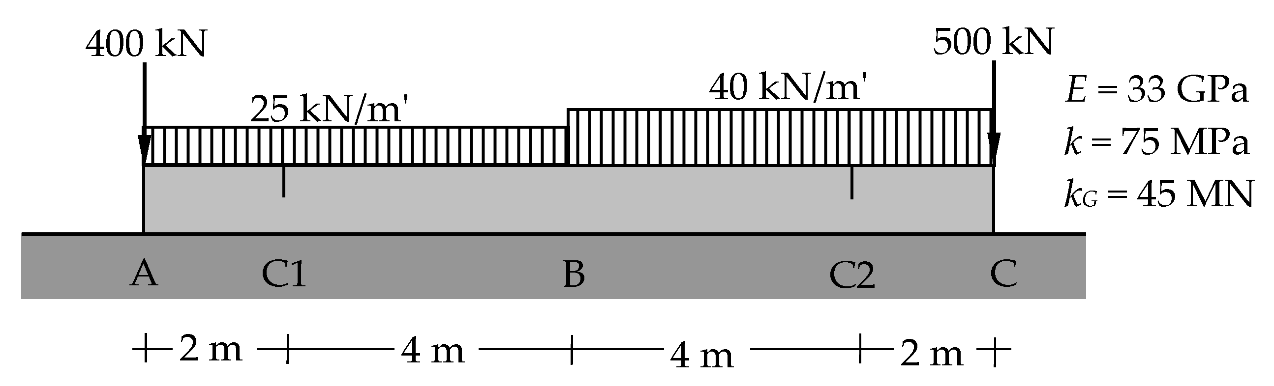
The examples setup is given in Figure 2. Both examples consider a beam with two transverse cracks of relative depth δ′ = 0.5 (with F(δ′ = 0.5) = 0.582914 obtained from Equation (2)), which are loaded with two uniformly distributed loads as well as with two transverse concentrated loads at both ends. The cross-section is a rectangle of width b = 0.5 m, while the heights of both examples differ: the values considered are h = 0.8 m and h = 0.1 m, respectively.

Figure 2.
Cracked beam resting on elastic soil.
At first, the solutions of corresponding governing differential equations (GDEs) were found just to obtain the benchmark values for both examples. The presence of two cracks and an in-field change of the applied transverse continuous load requires four elastic segments in the corresponding computational model of the beam. Consequently, four coupled differential equations were solved to obtain the model exact solutions. Afterwards, several FE meshes consisting completely of recently presented cb2psFE elements were analyzed, starting with the smallest model possible. Due to the presence of two cracks, two cb2psFE finite elements were required as a minimum.
4.1. First Example
In the first study, the rectangular cross-section height was taken as h = 0.8 m (with Kr = 2.76494∙108 Nm obtained from Equation (1)). This value led to the case where kG2 < 4·EIz·k, and both coefficients λ1 and λ2 were positive and real.
Therefore, the solutions obtained from the coupled system of GDEs were acquired the form of Equation (5):
In the initial FE model, the applied two-parametric soil stiffness matrices and load vectors obtained from Equations (25) and (29) of the implemented two cb2psFE of equal lengths were:
where all matrix components of the complete stiffness matrix [k1] obtained from Equations (22)–(24) are also shown for the first finite element.
Afterwards, element matrices, as well as load vectors, were assembled and three discrete nodal displacement values, as well as rotations, were calculated next. Subsequently, these discrete values were implemented with newly derived polynomial interpolation functions to obtain transverse displacement values between the nodes, as shown in Equations (8) and (9):
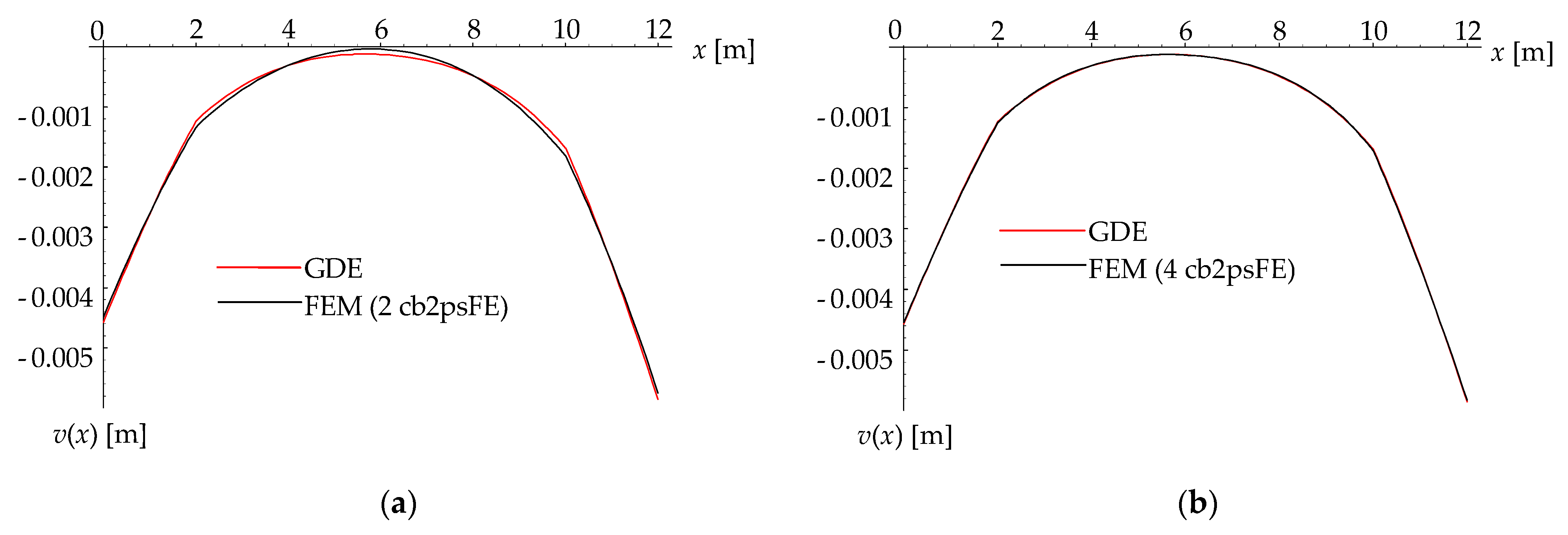
The results for transverse displacements are shown in Figure 3, where the horizontal axis represents the distance from the left end of the beam. The vertical axis shows the transverse displacement, and the red and black lines show the solutions of GDEs and the FEM model, respectively. It is clear from Figure 3a that both models exhibit decent agreement at the end nodes of the beam, but the discrepancies are more obvious at some other points. However, it should be noted that the implemented interpolation functions were polynomial interpolation functions, Equations (10) and (11), which do not include the genuine Winkler soil parameter.

Figure 3.
Comparison of transverse displacements for two (a) and four (b) FE meshes, respectively.
Nevertheless, mesh refinements had an obvious positive impact on the results as the differences between approximate solutions and the GDEs solutions effectively decreased. In Figure 3b, the results for transverse displacements are presented for the FEM computational model consisting of four cb2psFE elements of equal lengths (where for the non-cracked elements with δ′ = 0, the value of parameter ψ was taken as 0). The progress over the original two cb2psFE model is clearly evident as the discrepancies already almost vanished.
Furthermore, a comparison of displacements at five locations (points A, B, and C, which are located at the left end, mid-span, and right end, respectively, as well as both crack locations (C1 and C2)) for different finite element meshes is given in Table 1. While the discrete displacements of points A, B, and C of all meshes were obtained directly from the model system of linear equations, the displacement values at the crack locations (vC1 and vC2) were generally obtained by interpolation (denoted by * in the table). The only exceptions are meshes where the element node and the crack coincided in the model.

Table 1.
Results of transverse displacements for several solutions and locations.
Obviously, the comparison of displacement values in the table leads to the conclusion that the convergence of the results is evident. The values demonstrate that the directly obtained nodal values are generally slightly more accurate than the interpolated values between the nodes. However, it should be noted that the first soil parameter (i.e., k) is included solely in the calculation of the nodal displacement (through the newly presented stiffness matrices), while it is not included in the interpolation functions.
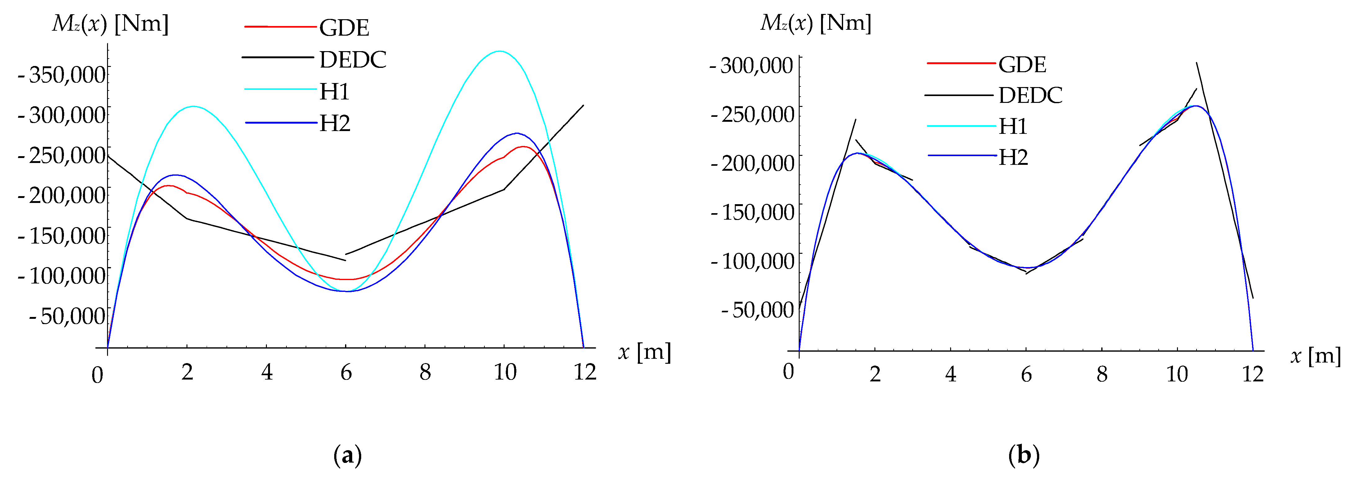
The discrete nodal displacements and rotations additionally allow for the matching nodal values of bending moments as well as shear forces to be calculated directly through the vector {Q}. By further implementations, these discrete values allow for bending moment functions to be calculated. Thus, Figure 4 shows the values of bending moment functions on the vertical axis obtained from the four implemented approaches, while the horizontal axis represents the distance from the left beam end. The red line shows the benchmark solutions of GDEs, while the black line shows the values obtained by DEDC i.e., through the second derivatives of transverse displacement functions. Furthermore, the light blue and the dark blue lines show the functions obtained from interpolations implementing H1 and H2 polynomials, respectively.

Figure 4.
Comparison of bending moments for two (a) and eight (b) FE meshes, respectively.
Figure 4a shows the results for the two FE meshes, and the impact of the degree of the polynomial is quite obvious as the fifth degree H2 polynomials evidently exhibit the best matching against the GDEs solutions. Nevertheless, if the mesh is refined and several more finite elements are applied, all discussed approaches converge toward exact GDEs solutions, however with different convergence rates. Thus, Figure 4b shows the results of eight finite element meshes. It is also evident from this figure that the agreement is increasing simultaneously with the degree of the implemented polynomial, although the differences between both Hermite polynomial solutions efficiently diminish.
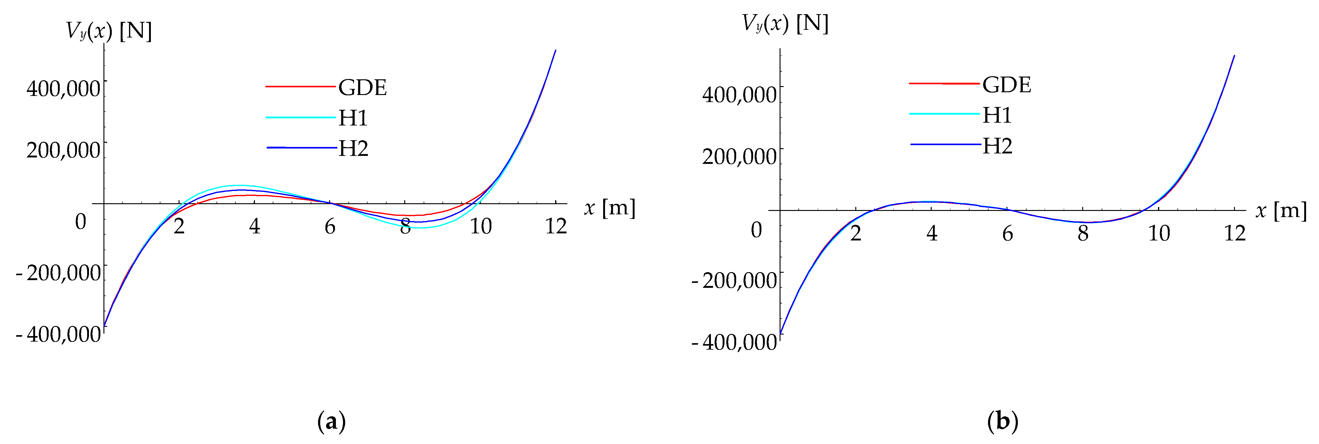
Among several approaches available for calculations of shear force functions, the direct interpolation of shear force values exhibited the optimal selection regarding the balance between the quality of the results and the computational efforts. Figure 5 on the vertical axis shows the shear force results for two (a) and four (b) cb2psFE meshes, respectively (the horizontal axis represents the distance from the left end of the beam). It confirms that even for a rather small number of finite elements, the H2 (as well as even H1) interpolation functions already produced excellent matching to the values obtained with the GDEs solutions.
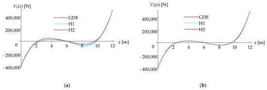
Figure 5.
Comparison of shear forces for two (a) and four (b) FE meshes, respectively.
4.2. Second Example
In this study, the height of the rectangular cross-section was reduced to h = 0.1 m (with Kr = 4.32022∙106 Nm obtained from Equation (1)). This value led to the case where kG2 > 4·EIz·k, consequently meaning that the coefficient λ2 became an imaginary value (such cases are possible in the engineering practice, although they are less frequent). This changed not only the numerical values of the coupled GDEs solutions but also their mathematical forms. Therefore, the corresponding solutions were obtained in the form of Equation (6):
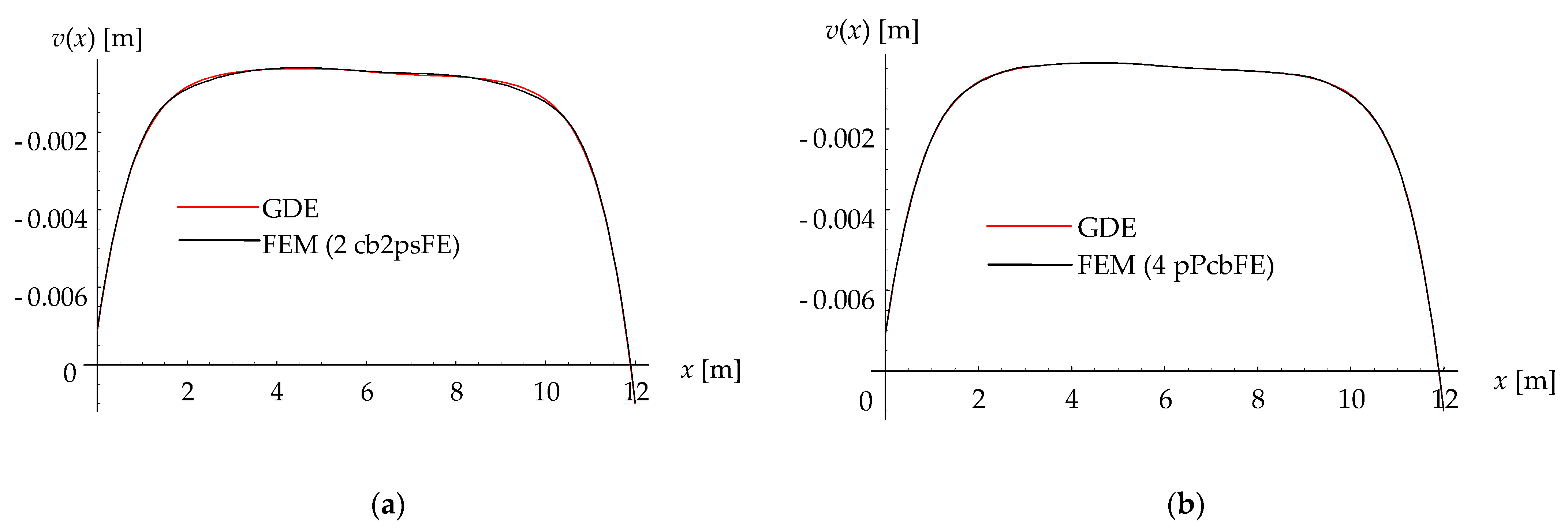
A two cb2psFE model was also applied here initially, whereas the corresponding stiffness matrices and load vectors were obtained from Equations (25) and (29), respectively. After solving the system of six linear equations, three discrete nodal displacement values as well as rotations were obtained. These values were further coupled with polynomial interpolation functions to additionally obtain transverse displacements between the nodes, as shown in Equations (8) and (9). This problem’s results for transverse displacements are presented in Figure 6. The abscissa axis represents the distance from the left end of the beam, and the ordinate axis represents the transverse displacement of the two models. In addition, the red and black lines show the solutions of GDEs and the cb2psFE model, respectively. It is apparent from Figure 6a that the results of the two FE mesh now exhibit almost perfect agreement at all three nodes and that only some rather small discrepancies are apparent in the vicinities of the cracks. Nevertheless, any discrepancies already completely disappear when four FEs are being implemented, as shown in Figure 6b.
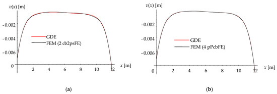
Figure 6.
Comparison of transverse displacements for two (a) and four (b) FE meshes, respectively.
Afterwards, several analyses with more finite elements were executed where the displacement curves of all models visually exhibited ideal matching with the GDEs solutions, as no discrepancies were detected. Therefore, just a comparison of displacements at five characteristic points for different finite element meshes is presented in Table 2.
Table 2.
Results of transverse displacements for several solutions and locations.
Figure 7 (in which the horizontal axis represents the distance from the left end of the beam, and the ordinate axis represents the bending moment) compares the bending moment values obtained by different approaches. As a result, it clearly shows the evolution of bending moment functions obtained from GDEs solutions (red line) as well as interpolated functions obtained by H1 (light blue) and H2 (dark blue) polynomials. It is undoubtedly evident from the figure that the GDEs bending moment functions are dominated by two extremely localized peaks near both beam ends (with intensive changes of curvature within their vicinities). Therefore, an increased number of finite elements (Ne) was required to obtain visually perfect agreement of the results (although some small discrepancies in the vicinities of the cracks remain still noticeable).

Figure 7.
Comparison of bending moments for various FE meshes: (a) Ne = 10; (b) Ne = 20; (c) Ne = 30; (d) Ne = 50.
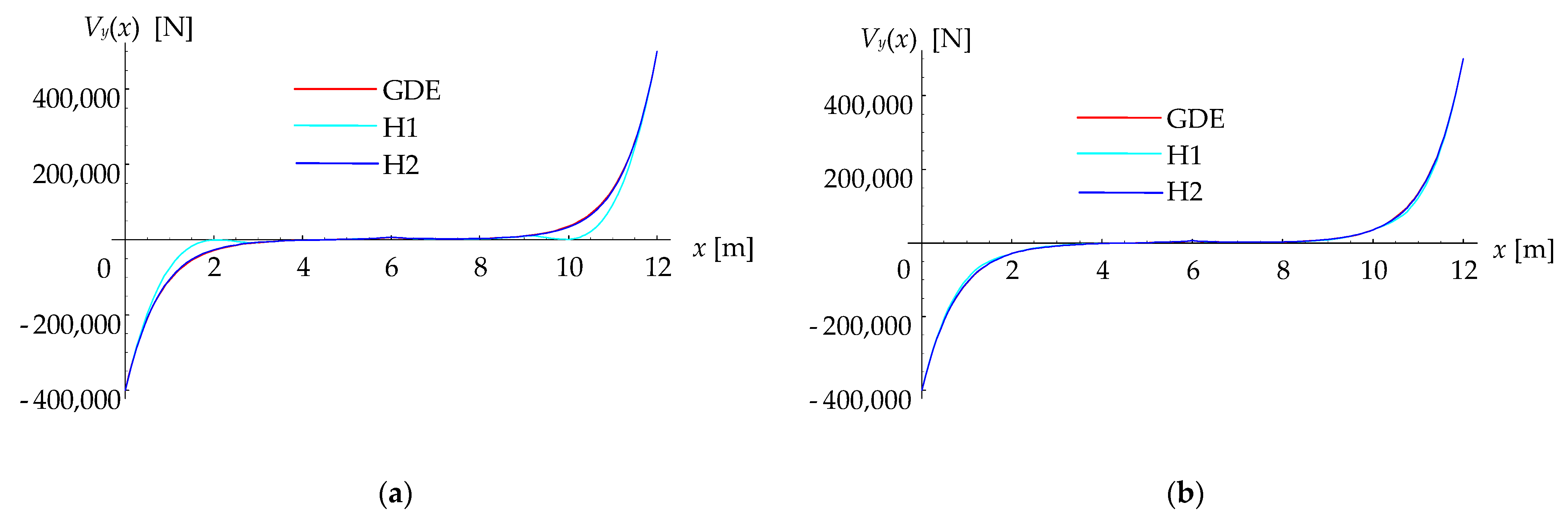
At last, functions of shear force distributions were calculated. Since these functions are smoother than the bending moment functions, fewer finite elements were required to obtain a very fine agreement of the results. The horizontal axis in Figure 8 represents the distance from the left end of the beam, and the vertical axis represents the results of the shear force. For a small number (i.e., four) of finite elements, as shown in Figure 8a, the H2 interpolation functions (dark blue) produced evidently better matching against GDEs solutions (red) as the H1 (light blue) interpolation functions. However, since the model number of FEs is actually governed by the bending moment functions, the differences between both interpolations became almost irrelevant with the increasing number of FEs as the H1 interpolation functions already produced good matching, as shown in Figure 8b.

Figure 8.
Comparison of shear function for four (a) and six (b) FE meshes, respectively.
5. Conclusions
The main conclusions can be summarized as follows:
- FEM bending analysis of slender cracked uniform beams resting on a two-parametric soil was considered.
- The second soil parameter was directly implemented in the new transverse displacement interpolation functions.
- The FE’s complete stiffness matrix consists of three separately derived matrices belonging to the beam and both soil contributions.
- The presented solutions converge to the exact differential equations solutions independently of the value of the coefficient λ2.
- Derived solutions in the closed symbolic form are applicable for all two-parametric soil models that have the same governing differential equation.
Nevertheless, future studies should initially focus on the inclusion of the first soil parameter directly in the interpolation functions (either in the form of approximate polynomials or by implementing exact solutions of the governing differential equations). Research could also consider variations of cross-sections and both soil parameters along the length of the element. The third research direction should be oriented toward experimental verifications.
Author Contributions
Conceptualization, M.S.; theory development and methodology, M.S.; software, M.S., D.I.; validation, M.S., D.I., M.U., I.P.; formal analysis, M.S., D.I.; writing—original draft preparation, M.S., D.I.; writing—review and editing, M.S., D.I., M.U., I.P.; visualization, M.S., D.I.; supervision, M.S., D.I.; project administration, M.S. All authors have read and agreed to the published version of the manuscript.
Funding
This research received no external funding.
Institutional Review Board Statement
Not applicable.
Informed Consent Statement
Not applicable.
Data Availability Statement
Data available on request from the authors.
Acknowledgments
The first author acknowledges the partial general financial support from the Slovenian Research Agency (research core funding No. P2-0129 (A) “Development, modelling and optimization of structures and processes in civil engineering and traffic”).
Conflicts of Interest
The authors declare no conflict of interest.
References
- Okamura, H.; Liu, H.-W.; Chu, C.-S.; Liebowitz, H. A Cracked Column under Compression. Eng. Fract. Mech. 1969, 1, 547–564. [Google Scholar] [CrossRef]
- Skrinar, M. A Finite Element of a Cracked Prismatic Beam on Elastic Foundation. Geotech. Eng. Transp. Syst. Environ. Prot. Proc. 1995, 2, 409–414. [Google Scholar]
- Skrinar, M.; Lutar, B. Analysis of Cracked Slender-Beams on Winkler’s Foundation, Using a Simplified Computational Model. Acta Geotech. Slov. 2011, 8, 5–17. [Google Scholar]
- Alijani, A.; Abadi, M.M.; Darvizeh, A.; Abadi, M.K. Theoretical Approaches for Bending Analysis of Founded Euler–Bernoulli Cracked Beams. Arch. Appl. Mech. 2018, 88, 875–895. [Google Scholar] [CrossRef]
- De Rosa, M.A.; Lippiello, M. Closed-Form Solutions for Vibrations Analysis of Cracked Timoshenko Beams on Elastic Medium: An Analytically Approach. Eng. Struct. 2021, 236, 111946. [Google Scholar] [CrossRef]
- Winkler, E. Die Lehre von Der Elasticitaet Und Festigkeit: Mit Besonderer Rücksicht Auf Ihre Anwendung in Der Technik, Für Polytechnische Schulen, Bauakademien, Ingenieure, Maschinenbauer, Architecten, Etc.; Verlag von H. Dominicus: Prague, Czech Republic, 1867. [Google Scholar]
- Skrinar, M.; Imamović, D. Exact Closed-form Finite Element Solution for the Bending Static Analysis of Transversely Cracked Slender Elastic Beams on Winkler Foundation. Int. J. Numer. Anal. Methods Geomech. 2018, 42, 1389–1404. [Google Scholar] [CrossRef]
- Selvadurai, A.P. Elastic Analysis of Soil-Foundation Interaction; Elsevier: Amsterdam, The Netherlands, 2013; ISBN 0-444-59628-3. [Google Scholar]
- Ostachowicz, W.M.; Krawczuk, M. Vibration Analysis of a Cracked Beam. Comput. Struct. 1990, 36, 245–250. [Google Scholar] [CrossRef]
- Liang, R.Y.; Hu, J.; Choy, F. Theoretical Study of Crack-Induced Eigenfrequency Changes on Beam Structures. J. Eng. Mech. 1992, 118, 384–396. [Google Scholar] [CrossRef]
- Hasan, W.M. Crack Detection from the Variation of the Eigenfrequencies of a Beam on Elastic Foundation. Eng. Fract. Mech. 1995, 52, 409–421. [Google Scholar] [CrossRef]
- Sundermeyer, J.N.; Weaver, R.L. On Crack Identification and Characterization in a Beam by Non-Linear Vibration Analysis. J. Sound Vib. 1995, 183, 857–871. [Google Scholar] [CrossRef]
- Ma, X.; Butterworth, J.W.; Clifton, G.C. Static Analysis of an Infinite Beam Resting on a Tensionless Pasternak Foundation. Eur. J. Mech. A/Solids 2009, 28, 697–703. [Google Scholar] [CrossRef]


Publisher’s Note: MDPI stays neutral with regard to jurisdictional claims in published maps and institutional affiliations. |
© 2021 by the authors. Licensee MDPI, Basel, Switzerland. This article is an open access article distributed under the terms and conditions of the Creative Commons Attribution (CC BY) license (https://creativecommons.org/licenses/by/4.0/).