Line Scan Spatial Speckle Contrast Imaging and Its Application in Blood Flow Imaging

Abstract

Laser speckle imaging has been an indispensable tool for visualizing blood flow in biomedical applications. We proposed a novel design of the laser speckle imaging system, which combines confocal illumination and detection with various speckle analysis methods. The system can be operated by three imaging modes. One is surface illumination laser speckle contrast imaging (SI-LSCI) and the other two are line scan temporal speckle contrast imaging (LS-TSCI) and line scan spatial speckle contrast imaging (LS-SSCI). The experimental results of flow phantoms have validated the mixture model, which combines the Lorentzian and Gaussian models to describe the simultaneous existence of both Brownian motions and ordered flow. Our experimental results of in vivo chick embryos demonstrate that LS-SSCI maintains high temporal resolution and is less affected by motion artifacts. LS-SSCI can provide better image quality for in vivo imaging blood chick embryos than LS-TSCI. Furthermore, the experiential results present that LS-SSCI can detect and quantify the blood flow change during vascular clipping, and shows great potential in diagnosing vascular diseases, such as angiosclerosis, angiostenosis, or angiemphraxis.

1. Introduction

Laser speckle contrast imaging (LSCI) has been broadly applied to visualize blood flow imaging in living tissues, such as the retina [1,2,3,4], skin [5,6,7,8,9], and brain [10,11,12,13,14,15,16] since it was first introduced in the 1980s [1]. It can monitor the dynamic blood flow response and relative changes in values. A few reviews have summarized the recent technological advancements and some practical challenges of LSCI [17,18,19,20,21]. Fercher and Briers firstly studied the quantitative relationship between the contrast of speckle pattern and the velocity of the flow, and assumed a Lorentzian distribution for Brownian motion (unordered flow) of the scatterers [1]. In fact, some research groups demonstrated that the Lorentzian model is suitable for Brownian motion [1,22,23,24]. The Gaussian model is generally considered more suitable for ordered flow [23,25,26]. Many researchers often discuss which model is more appropriate [22,26,27,28,29,30]. Liu et al. [31] analyzed the influence of the assumptions in the LSCI theory on the accuracy of blood flow estimation. They proved that the blood flow changes are severely underestimated by the most commonly used LSCI model under ischemic conditions, and proposed an alternative model that can measure blood flow changes more accurately. Tarantini et al. [32] demonstrated that the influence of anti-aging or anti-AD treatments on cerebral micro vascular health can be evaluated by LSCI. Zheng et al. [33] developed a dual-display laparoscopic vision system, which combines LSCI with a commercially rigid laparoscope. The standard color vision, unlabeled vasculature imaging, and fusion display modes are available. They found that the integrated system can detect early changes in bowel perfusion that are invisible with standard color imaging. Parthasarathy et al. [34] proved that LSCI is capable of generating real-time full field cerebral blood flow images with high spatial resolution, while minimizing damage to the surgical process during neurosurgeries.

However, conventional LSCI is based on wide-field optical imaging, which suffers from deteriorated spatial resolution and contrast when the sample is optically thick. In a previous paper, line scan laser speckle contrast imaging (LS-LSCI) was proven with good experimental results with higher spatial resolution than conventional laser speckle contrast imaging [35,36]. In this paper, we further compared the performance of spatial and temporal speckle contrast-based image acquisition approaches, and verified the flow quantification capability of our speckle imaging system, which features confocal illumination and detection. The system can be configured with three imaging modes. The first one is surface illumination laser speckle contrast imaging (SI-LSCI), and the other two are line scan temporal speckle contrast imaging (LS-TSCI) and line scan spatial speckle contrast imaging (LS-SSCI). The Materials and Method section discloses the imaging setup, theoretical models, data processing, and sample preparation details. The Results and Discussion section presents the experimental images obtained from chick embryos, and compared and fully discussed the performance of various imaging modes.

2. Materials and Methods

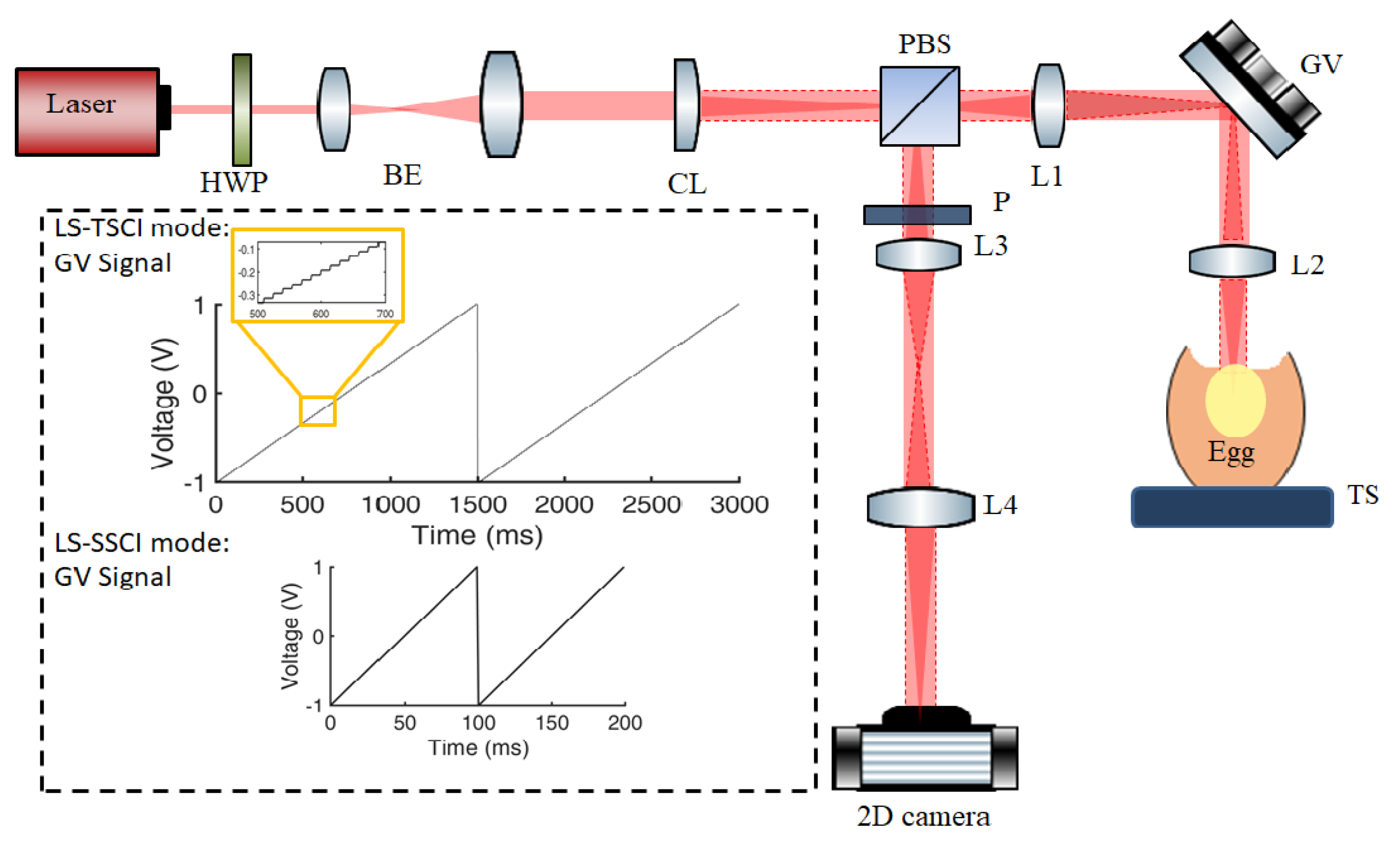
2.1. Experimental Setup

Figure 1 shows the layout of our laser speckle imaging. The details of the experimental setup are described in our previous publication [35]. The light source was a 640 nm single-frequency laser with 25 mW. The laser intensity illuminated on the sample can be controlled by the half-wave plate (HWP) and polarizing beam-splitter (PBS). A cylindrical lens was used to focus the light in 1-D and generate an illumination line. A 1-D galvo mirror was used to scan the illumination line across the sample. The backscattered photons from the sample were de-scanned by the same galvo mirror and captured by the camera (Andor, Zyla 5.5, scientific CMOS). The camera supports both global shutter and rolling shutter. It has two operation modes. One is the traditional 2D camera mode for surface illumination laser speckle contrast imaging (SI-LSCI) without the cylindrical lens in the light path, and the galvo mirror is set at a stationary position without scanning. The other is operated as the line camera for the line scan laser speckle contrast imaging. Additionally, based on the current setup, we are also able to obtain the morphological images. A white light source (Leica CLS 150 XE) is used to form a uniform illuminated area to obtain the conventional morphological microscope images.

Particularly, different from previous acquisition modes, the system has been upgraded to three imaging modes. One is surface illumination laser speckle contrast imaging (SI-LSCI). The other two are line scan temporal speckle contrast imaging (LS-TSCI) and line scan spatial speckle contrast imaging (LS-SSCI). As illustrated in the black dashed box in Figure 1, in LS-TSCI mode, the galvo mirror is driven by a periodic stair-step waveform; in LS-SSCI mode, the galvo mirror is driven by a periodic sawtooth wave signal, which varies linearly with time in each frame period. Both in LS-TSCI and LS-SSCI mode, the sensing element of the camera is conjugated to the illumination line. In LS-TSCI mode, assuming that the number of steps per frame is 100 and the width of each step is 15 with the exposure time 1 ms, 15 consecutive raw speckle intensity data can be used to calculate one temporal speckle contrast. Thus, it will take 1500 ms to acquire one speckle image. In LS-SSCI mode, assuming that the number of lines per frame is 100 and the integral time of line camera is 1 ms, it will take 100 ms to obtain one speckle image. In the experiments, a data acquisition board (NI, PCI-6115) was used to produce both the trigger signals and the driving waveform of the galvo mirror to synchronize the galvo mirror to the camera. We designed a homemade LabVIEW program for hardware control and image acquisition.

2.2. Theory

The speckle contrast is computed by the ratio of the standard deviation to the mean intensity, is expressed as,

$$K=\frac{\sigma }{\langle I\rangle }$$

(1)

where σ_t refers to the temporal standard deviation and K_t is the temporal speckle contrast. Similarly, the spatial speckle contrast (K_s) can be expressed as the ratio of spatial standard deviation (σ_s) to the mean intensity <I>. The speckle contrast (K) is a function of the correlation time τ and the exposure time T of the camera as [28].

$$K^2=\frac{1}{T}{\displaystyle \underset{0}{\overset{T}{\int }}\beta {\left|g_1(\tau )\right|}^2\left[2(1-\frac{\tau }{T})\right]d\tau }$$

(2)

where β ≤ 1 is a parameter related to the loss of correlation and g₁(τ) is the field autocorrelation function. For Brownian motion (unordered flow), the field autocorrelation function g₁(τ) corresponds to a Lorentzian line shape, which can be expressed as [30]

$$|g_{1,Brownian}(\tau ){|}^2=\exp (-2\tau /{\tau }_{c,Brownian})$$

(3)

For ordered flow, the field autocorrelation function g₁(τ) corresponds to a Gaussian line shape, which can be expressed as [30]

$$|g_{1,ordered}(\tau ){|}^2=\exp (-2{(\tau /{\tau }_{c,ordered})}^2)$$

(4)

Duncan and Kirkpatrick have pointed out that the actual distribution is some combination of the two models [30]. In this paper, we assume that the field autocorrelation function g₁(τ) can be expressed as:

$$|g_1(\tau ){|}^2=\exp (-2\tau /{\tau }_{c,Brownian})\times \exp (-2{(\tau /{\tau }_{c,ordered})}^2)$$

(5)

Therefore, In the case of only Brownian motion, using the Equations (3) and (2), speckle contrast is given by

$$K=\sqrt{\frac{1}{T}{\displaystyle \underset{0}{\overset{T}{\int }}\beta \exp (-2\tau /{\tau }_{c,Brownian})\left[2(1-\frac{\tau }{T})\right]d\tau }}$$

(6)

In the case of both Brownian motion and ordered flow, using the Equations (5) and (2), speckle contrast is given by

$$K=\sqrt{\frac{1}{T}{\displaystyle \underset{0}{\overset{T}{\int }}\beta \exp (-2\tau /{\tau }_{c,Brownian})\times \exp (-2{(\tau /{\tau }_{c,ordered})}^2)\left[2(1-\frac{\tau }{T})\right]d\tau }}$$

(7)

2.3. Data Processing

As mentioned in Section 2.2, the temporal speckle contrast K can be calculated as [12].

$$K_t=\frac{{\sigma }_t}{\langle I\rangle }=\frac{\sqrt{\frac{{\displaystyle {\sum }_{i=1}^N{(I_i-\langle I\rangle )}^2}}{N-1}}}{\langle I\rangle }=\frac{\sqrt{\frac{N{\displaystyle {\sum }_{i=1}^N{I}_{{}_i}^2-{({\displaystyle {\sum }_{\mathrm{i}=1}^N{I}_i})}^2}}{N(N-1)}}}{\frac{{\displaystyle {\sum }_{\mathrm{i}=1}^N{I}_i}}{N}}$$

(8)

Note that i refers to the index of raw laser speckle image in the sequence. N is the total number of speckle images. I_i is the intensity of the captured i-th speckle image. In this paper, 15 consecutive frames are captured by the camera and can be calculated to the temporal speckle contrast using Equation (8).

The spatial speckle contrast K can be computed as [20].

$$\begin{array}{l}{K}_{i,j}=\frac{{\sigma }_{\mathrm{s}}}{{\langle I\rangle }_s},\\ {\langle I\rangle }_s=\frac{{\displaystyle \sum _{x=i-(m-1)/2}^{i+(m-1)/2}{\displaystyle \sum _{y=j-(m-1)/2}^{j+(m-1)/2}{I}_{x,y}}}}{m^2}\\ {\sigma }_{\mathrm{s}}=\sqrt{\frac{{\displaystyle \sum _{x=i-(m-1)/2}^{i+(m-1)/2}{\displaystyle \sum _{y=j-(m-1)/2}^{j+(m-1)/2}{(I_{x,y}-\langle I\rangle )}^2}}}{m^2}}\end{array}$$

(9)

Note that K_i,j is assigned to the central pixel in the coordinates (i, j) and a sliding m × m pixel window is used to compute the spatial standard deviation (σ_s) and the mean intensity <I>. Moving the K_i,j element along the x and y direction can calculate a spatial speckle contrast 2-D map. In this paper, LS-SSCI was computed using a typical square sliding window of 7 × 7 pixels followed by averaging 15 time points to compare the LS-TSCI.

2.4. Flow Phantom

The flow phantom consisted of lipofundin MCT/LCT (4%) solutions (B.Braun Melsungen AG, Germany) in a polyethylene tube driven by a digital syringe pump (SPLab01, Baoding Shenchen Precision Pump Co., Ltd., Baoding, China) at a steady flow rate from 0 to 10 mm/s.

2.5. Sample Preparation

Chick embryos have been widely used as small animal models for microvascular research. We purchased the fertilized chick eggs from a local poultry farm (Lian Wah Hang Farm PTE Ltd., Singapore). The incubation temperature of eggs is 37–38 °C, and humidity is 70–80%. On the 3rd day of the embryo, the eggs can be seen by making a hole in the shell and removing the covered membranes. The eggs were then placed on the sample holder and ready for imaging. All the experiments were conducted with the review and approval of the Institutional Animal Care and Use Committee (IACUC) of National University of Singapore.

3. Results and Discussion

3.1. Validation of Line Scan Laser Speckle Contrast Imaging

To validate the line scan laser speckle contrast imaging method with theoretical models, flow phantoms were studied. Figure 2 illustrates the temporal speckle contrast K of the flow phantom varies with different exposure times under different flow velocities using LS-TSCI setup with a special configuration. The galvo mirror was set at a stationary position without scanning, and temporal speckle contrasts were obtained from the continuously acquired line patterns. As shown in Figure 2, the temporal speckle contrast K values are plotted for unordered Brownian motion and different directional flow velocities. Firstly, the Brownian motion (0 mm/s) experimental data are fitted to Equation (6) (Lorentzian autocorrelation function) with β = 1. They show that the Lorentzian model is in good agreement with the experimental results, the correlation time of speckles τ_c,Brownian is estimated at 1.3 ms as a fitting parameter. Then, the directional flow experimental data are fitted to Equation (7) (Combined model) with τ_c,Brownian = 1.3 ms, β = 1. The fitting results are in good agreement with the experimental measurements. The obtained fitting parameter τ_c,ordered is reduced from 1.1 ms for 0.35 mm/s to 68 µs for 10 mm/s. As shown in Figure 3, 1/τ_c,ordered is linear with the flow velocity (r² = 0.9905). The experimental results verified that the correlation time τ_c,ordered is in inverse proportion to the flow velocity of the scattering particles [28].

3.2. Choose the Appropriate Integration Time for Blood Flow Imaging of Chick Embryo

The exposure time is a freely selectable parameter, but the choice of the integration time has a great influence on the calculated contrast values (shown in Figure 4). To choose the proper integration time for imaging the blood flow of chick embryos, multi-exposure laser speckle contrast imaging was studied. Figure 4 shows the temporal speckle contrast images of a chick embryo (NO.1 day 3) obtained with the SI-LSCI at different exposure durations of 0.1, 0.2, 0.5, 1, 2, 4, 6, and 10 ms, respectively. All speckle contrast images in Figure 4 are obtained by imaging the same region of the chick embryo. With a short exposure durations of 0.2 ms (Figure 4b), the laser speckle contrast image shows the blood vessels with fast flow velocity around the heart. Meanwhile, with a shorter exposure duration of 0.1 ms (Figure 4a), the contrast image shows nothing. The vessels are invisible in the image. With a longer exposure duration of 10 ms (Figure 4h), the speckle contrast image highlights the blood vessels with slower flow velocity further away from the heart. The experimental results demonstrated that the smaller vessels, which have a lower flow velocity, become more apparent with the increasing exposure time. A quantitative analysis is provided in Figure 4i, where the relative noise σ_K/K in the speckle contrast images is plotted as a function of the exposure time. It shows that the image noise at the exposure time 4 ms is very close to that of 10 ms. Therefore, 4 ms is a near-optimal compromise between the image quality and the image acquisition speed for LS-TSCL and LS-SSCI.

3.3. Comparison of LS-TSCI and LS-SSCI

After the optimum exposure time was determined, we compared the performances of LS-TSCI and LS-SSCI. Figure 5a,b shows the temporal speckle contrast image and spatial speckle contrast image of chick embryo (day 3.5, NO. 2) using LS-TSCI and LS-SSCI at line exposure durations of 4 ms, respectively. The results demonstrate that LS-TSCI and LS-SSCI were essentially identical, but due to the poor temporal resolution, LS-TSCI is sensitive to motion artifacts due to heartbeats, particularly around the heart, dorsal aorta, and artery (shown in Figure 5a). Though spatial sampling in LS-SSCI reduces the spatial resolution, LS-SSCI maintains high temporal resolution, and is less affected by motion artifacts. Consequently, LS-SSCI can provide better image quality for the in vivo imaging blood flow of chick embryos than LS-TSCI.

3.4. Imaging Blood Flow Changes during Vascular Clipping Using LS-SSCI

LS-SSCI was employed to observe blood flow changes during the vascular clipping of chick embryos. Chick embryo (day 3, NO. 3) was used for the experiment. A silk suture (Ethicon, w1814, shown in Figure 6c using the red circle) was used for the vascular clipping. Figure 6a,c shows the wide-field image with white light illumination before and after the clipping, respectively. Figure 6b,d shows the corresponding speckle contrast image using LS-SSCI before and after the vascular clipping, respectively. The difference between Figure 6b,d is illustrated in the figures using the yellow circles. The vessel in the yellow region indicated in Figure 6b can be clearly seen, but this vessel is invisible in Figure 6d. The observations demonstrated that the clipping caused a severe reduction in blood flow in the regions of almost 100%. The experimental results proved that LS-SSCI shows great potential in diagnosing vascular diseases, such as angiosclerosis, angiostenosis, or angiemphraxis.

4. Conclusions

In summary, we have upgraded the laser speckle imaging system, which consists of three imaging modes and can be switched flexibly and instantly. The first one is surface illumination laser speckle contrast imaging (SI-LSCI), and the other two are line scan temporal speckle contrast imaging (LS-TSCI) and line scan spatial speckle contrast imaging (LS-SSCI). We validated the combined model of Lorentzian and Gaussian line shapes by the flow phantoms. Using SI-LSCI, we experimentally studied the speckle contrast varied with the exposure time. The experimental results suggested 4 ms is a proper exposure time for imaging the blood flow of chick embryos. To compare the performance of LS-TSCI and LS-SSCI, chick embryos imaging experiments were conducted. The experimental results demonstrated that LS-SSCI, which maintains high temporal resolution and is less affected by motion artifacts, can provide better image quality for in vivo imaging blood flow of chick embryos than LS-TSCI. Furthermore, we applied LS-SSCI to measure blood flow change during the vascular clipping of chick embryos. LS-SSCI shows great potential in diagnosing vascular diseases such as angiosclerosis, angiostenosis, or angiemphraxis.

References

1. Fercher, A.; Briers, J. Flow visualization by means of single-exposure speckle photography. Opt. Commun. 1981, 37, 326–330. [Google Scholar] [CrossRef]
2. Briers, J.D.; Fercher, A.F. Retinal blood-flow visualization by means of laser speckle photography. Investig. Ophthalmol. Vis. Sci. 1982, 22, 255–259. [Google Scholar]
3. Tamaki, Y.; Araie, M.; Kawamoto, E.; Eguchi, S.; Fujii, H. Noncontact, two-dimensional measurement of retinal microcirculation using laser speckle phenomenon. Investig. Ophthalmol. Vis. Sci. 1994, 35, 3825–3834. [Google Scholar]
4. Cheng, H.; Yan, Y.; Duong, T.Q. Temporal statistical analysis of laser speckle images and its application to retinal blood-flow imaging. Opt. Express 2008, 16, 10214–10219. [Google Scholar] [CrossRef] [Green Version]
5. Huang, Y.-C.; Ringold, T.L.; Nelson, J.S.; Choi, B. Noninvasive blood flow imaging for real-time feedback during laser therapy of port wine stain birthmarks. Lasers Surg. Med. 2008, 40, 167–173. [Google Scholar] [CrossRef] [PubMed] [Green Version]
6. Choi, B.; Kang, N.M.; Nelson, J. Laser speckle imaging for monitoring blood flow dynamics in the in vivo rodent dorsal skin fold model. Microvasc. Res. 2004, 68, 143–146. [Google Scholar] [CrossRef] [Green Version]
7. Roustit, M.; Millet, C.; Blaise, S.; Dufournet, B.; Cracowski, J. Excellent reproducibility of laser speckle contrast imaging to assess skin microvascular reactivity. Microvasc. Res. 2010, 80, 505–511. [Google Scholar] [CrossRef] [PubMed]
8. Mahé, G.; Humeau-Heurtier, A.; Durand, S.; Leftheriotis, G.; Abraham, P. Assessment of skin microvascular function and dysfunction with laser speckle contrast imaging. Circ. Cardiovasc. Imaging 2012, 5, 155–163. [Google Scholar] [CrossRef] [Green Version]
9. Mirdell, R.; Farnebo, S.; Sjöberg, F.; Tesselaar, E. Accuracy of laser speckle contrast imaging in the assessment of pediatric scald wounds. Burns 2018, 44, 90–98. [Google Scholar] [CrossRef] [Green Version]
10. Dunn, A.K.; Bolay, H.; Moskowitz, M.A.; Boas, D.A. Dynamic Imaging of Cerebral Blood Flow Using Laser Speckle. Br. J. Pharmacol. 2001, 21, 195–201. [Google Scholar] [CrossRef] [Green Version]
11. Bolay, H.; Reuter, U.; Dunn, A.K.; Huang, Z.; Boas, D.A.; Moskowitz, M.A. Intrinsic brain activity triggers trigeminal meningeal afferents in a migraine model. Nat. Med. 2002, 8, 136–142. [Google Scholar] [CrossRef]
12. Li, P.; Ni, S.; Zhang, L.; Zeng, S.; Luo, Q. Imaging cerebral blood flow through the intact rat skull with temporal laser speckle imaging. Opt. Lett. 2006, 31, 1824–1826. [Google Scholar] [CrossRef] [PubMed]
13. Shin, H.K.; Dunn, A.K.; Jones, P.B.; A Boas, D.; A Moskowitz, M.; Ayata, C. Vasoconstrictive neurovascular coupling during focal ischemic depolarizations. Br. J. Pharmacol. 2005, 26, 1018–1030. [Google Scholar] [CrossRef] [Green Version]
14. Zakharov, P.; Völker, A.C.; Wyss, M.T.; Haiss, F.; Calcinaghi, N.; Zunzunegui, C.; Buck, A.; Scheffold, F.; Weber, B. Dynamic laser speckle imaging of cerebral blood flow. Opt. Express 2009, 17, 13904–13917. [Google Scholar] [CrossRef] [PubMed] [Green Version]
15. Dunn, A.K. Laser speckle contrast imaging of cerebral blood flow. Ann. Biomed. Eng. 2011, 40, 367–377. [Google Scholar] [CrossRef] [PubMed] [Green Version]
16. Chen, M.; Wen, D.; Huang, S.; Gui, S.; Zhang, Z.; Lu, J.; Li, P. Laser speckle contrast imaging of blood flow in the deep brain using microendoscopy. Opt. Lett. 2018, 43, 5627–5630. [Google Scholar] [CrossRef]
17. Boas, D.A.; Dunn, A.K. Laser speckle contrast imaging in biomedical optics. J. Biomed. Opt. 2010, 15, 011109. [Google Scholar] [CrossRef] [Green Version]
18. Senarathna, J.; Rege, A.; Li, N.; Thakor, N.V. Laser speckle contrast imaging: Theory, instrumentation and applications. IEEE Rev. Biomed. Eng. 2013, 6, 99–110. [Google Scholar] [CrossRef]
19. Briers, D.; Duncan, D.D.; Hirst, E.; Kirkpatrick, S.J.; Larsson, M.; Steenbergen, W.; Stromberg, T.; Thompson, O.B. Laser speckle contrast imaging: Theoretical and practical limitations. J. Biomed. Opt. 2013, 18, 066018. [Google Scholar] [CrossRef] [Green Version]
20. Vaz, P.G.; Humeau-Heurtier, A.; Figueiras, E.; Correia, C.; Cardoso, J.M. Laser speckle imaging to monitor microvascular blood flow: A review. IEEE Rev. Biomed. Eng. 2016, 9, 106–120. [Google Scholar] [CrossRef] [Green Version]
21. Heeman, W.; Steenbergen, W.; Van Dam, G.M.; Boerma, E.C. Clinical applications of laser speckle contrast imaging: A review. J. Biomed. Opt. 2019, 24, 080901. [Google Scholar] [CrossRef] [PubMed] [Green Version]
22. Draijer, M.; Hondebrink, E.; van Leeuwen, T.; Steenbergen, W. Review of laser speckle contrast techniques for visualizing tissue perfusion. Lasers Med. Sci. 2008, 24, 639–651. [Google Scholar] [CrossRef] [PubMed] [Green Version]
23. Ramirez-San-Juan, J.C.; Nelson, J.S.; Choi, B. Comparison of lorentzian and guassian-based approaches for laser speckle imaging of blood flow dynamics. In Coherence Domain Optical Methods and Optical Coherence Tomography in Biomedicine X; Tuchin, V.V., Izatt, J.A., Fujimoto, J.G., Eds.; SPIE: Bellingham, WA, USA, 2006; Volume 6079, pp. 380–383. [Google Scholar]
24. Duncan, D.D.; Kirkpatrick, S.J.; Gladish, J.C. What is the proper statistical model for laser speckle flowmetry? In Complex Dynmics and Fluctuations in Biomedical Photonics; SPIE: Bellingham, WA, USA, 2008; Volume 6855, p. 685502. [Google Scholar]
25. Briers, J.; Webster, S. Quasi real-time digital version of single-exposure speckle photography for full-field monitoring of velocity or flow fields. Opt. Commun. 1995, 116, 36–42. [Google Scholar] [CrossRef]
26. Ramirez-San-Juan, C.; Ramos-García, R.; Guizar-Iturbide, I.; Martínez-Niconoff, G.; Choi, B. Impact of velocity distri-bution assumption on simplified laser speckle imaging equation. Opt. Express 2008, 16, 3197–3203. [Google Scholar] [CrossRef] [PubMed] [Green Version]
27. Wang, Z.; Hughes, S.M.; Dayasundara, S.; Menon, R.S. Theoretical and experimental optimization of laser speckle contrast imaging for high specificity to brain microcirculation. Br. J. Pharmacol. 2006, 27, 258–269. [Google Scholar] [CrossRef]
28. Duncan, D.D.; Kirkpatrick, S.J. Can laser speckle flowmetry be made a quantitative tool? J. Opt. Soc. Am. A 2008, 25, 2088–2094. [Google Scholar] [CrossRef] [PubMed]
29. Parthasarathy, A.B.; Kazmi, S.M.S.; Dunn, A.K. Quantitative imaging of ischemic stroke through thinned skull in mice with Multi Exposure Speckle Imaging. Biomed. Opt. Express 2010, 1, 246–259. [Google Scholar] [CrossRef] [Green Version]
30. Nadort, A.; Woolthuis, R.G.; van Leeuwen, T.; Faber, D. Quantitative laser speckle flowmetry of the in vivo microcirculation using sidestream dark field microscopy. Biomed. Opt. Express 2013, 4, 2347–2361. [Google Scholar] [CrossRef] [Green Version]
31. Liu, C.; Kılıç, K.; Erdener, S.E.; Boas, D.A.; Postnov, D.D. Choosing a model for laser speckle contrast imaging. Biomed. Opt. Express 2021, 12, 3571–3583. [Google Scholar] [CrossRef]
32. Tarantini, S.; Fulop, G.A.; Kiss, T.; Farkas, E.; Zölei-Szénási, D.; Galvan, V.; Toth, P.; Csiszar, A.; Ungvari, Z.; Yabluchanskiy, A. Demonstration of impaired neurovascular coupling responses in TG2576 mouse model of Alzheimer’s disease using functional laser speckle contrast imaging. GeroScience 2017, 39, 465–473. [Google Scholar] [CrossRef] [Green Version]
33. Zheng, C.; Lau, L.W.; Cha, J. Dual-display laparoscopic laser speckle contrast imaging for real-time surgical assistance. Biomed. Opt. Express 2018, 9, 5962–5981. [Google Scholar] [CrossRef] [PubMed]
34. Parthasarathy, A.B.; Weber, E.L.; Richards, L.M.; Fox, D.J.; Dunn, A.K. Laser speckle contrast imaging of cerebral blood flow in humans during neurosurgery: A pilot clinical study. J. Biomed. Opt. 2010, 15, 066030. [Google Scholar] [CrossRef]
35. Du, E.; Shen, S.; Chong, S.P.; Chen, N. Multifunctional laser speckle imaging. Biomed. Opt. Express 2020, 11, 2007–2016. [Google Scholar] [CrossRef] [PubMed]
36. Du, E.; Shen, S.; Qiu, A.; Chen, N. Confocal laser speckle autocorrelation imaging of dynamic flow in microvasculature. Opto-Electron. Adv. 2021, in press. [Google Scholar]
Figure 1. Schematic of the experimental setup for laser speckle imaging: HWP, half-wave plate; BE, beam expander (3×); CL, cylindrical lens; PBS, polarizing beam splitter; GV, 1-D galvo mirror; P, polarizer. TS, translational stage. The focal lengths of CL, L1, L2, L3, and L4 were 50, 50, 75, 40, and 100 mm, respectively.
Applsci 11 10969 g001
Figure 2. Measured temporal speckle contrast of flow phantom (data points) and corresponding fitting results (solid lines) for different flow velocities using LS-TSCI setup.
Applsci 11 10969 g002
Figure 3. Dependence of fitting parameter τc,ordered (plotted as 1/τc,ordered) obtained from the speckle contrast and flow velocities. The linear correlation coefficient is 0.9905.
Applsci 11 10969 g003
Figure 4. (ah) Temporal laser speckle contrast image of a chick embryo (day 3) obtained with the SI-LSCI at different exposure durations 0.1, 0.2, 0.5, 1, 2, 4, 6, and 10 ms, respectively. (i) Relative noise in the speckle contrast image σK /K at different exposure times.
Applsci 11 10969 g004
Figure 5. The laser speckle contrast images of a chick embryo (day 3.5) under the exposure time 4 ms using the (a) LS-TSCI; (b) LS-SSCI. The image area is 10.24 mm × 8.64 mm.
Applsci 11 10969 g005
Figure 6. (a) A wide-field image of the chick embryo (day 3) with white light illumination. (b) The corresponding laser speckle contrast image using LS-SSCI before clipping. (c) The intensity image of the same chick embryo after vascular clipping. The silk suture is indicated in the red circle. (d) The corresponding laser speckle contrast image using LS-SSCI after clipping. The vessel in the yellow circle is more visible in (b) compared to (d). The image area is 4.26 mm × 6.78 mm.
Applsci 11 10969 g006
Publisher’s Note: MDPI stays neutral with regard to jurisdictional claims in published maps and institutional affiliations.