Conceptual Solution Decision Based on Rough Sets and Shapley Value for Product-Service System: Customer Value-Economic Objective Trade-Off Perspective

Abstract

The product service system (PSS), as a design concept for integrated products and services, needs to be evaluated in the early design stage to maximize the value for stakeholders of the PSS concept, which is a crucial task for enterprises. However, existing methods focus on the ranking and value assessment of PSS evaluation criteria (e.g., quality, sustainability, cost), ignoring the needs conflict between customer value and economic objectives in PSS design, resulting in decision results that are not applicable to industrial enterprises. Furthermore, the influence of weight preference and uncertain information on solution evaluation is seldom considered when calculating the weight of each criterion. To fill this gap, integrating rough sets and the Shapley value decision approach for product-service system design considering customer value-economic objective trade-off is proposed, which mainly includes two parts: firstly, the best worst method (BWM) and the entropy weight method are integrated to obtain the comprehensive weight of evaluation criteria in the customer value and economic objectives; secondly, the Shapley value method in the coalition game is used to solve the optimal expectation allocation of the two objectives, so as to select the solution closest to the allocation, i.e., the optimal solution. In addition, rough set techniques are used to capture and integrate subjective assessment information originating from DMs under uncertainty. Finally, a case study of the electric forklift design is illustrated to verify the proposed decision model. The decision results show that this approach is more reliable through sensitivity and comparison analysis, and provide a valuable recommendation for enterprises to consider product service in forklift design.

1. Introduction

The product service system (PSS) is a design approach that combines products with services, which is widely adopted in the transformation of manufacturing enterprises to enhance product competitiveness [1,2]. By considering the multidimensional nature of PSS design, the PSS has the potential to create synergies between user needs and corporate profits that cannot be obtained by focusing only on the service performance (e.g., sustainability, serviceability) or more traditional objectives (e.g., time, quality) in product development [3]. Furthermore, PSS provides customers with integrated solutions of products and services, and provides personalized services according to different user needs, so as to improve customer satisfaction [4]. The PSS design cycle comprises a large number of design factors and data [5], which can be used to identify customer requirements and evaluate PSS conceptual solutions. However, excessive focus on customer demands may lead to designs that are too expensive to be implemented as actual industrial products. For example, there are conflicting needs between users’ service performance of the product and the product lifecycle cost of the enterprises, which may increase the burdens for enterprises to improve the serviceability of PSS design. For this reason, to satisfy the customer service needs of the product in the PSS design and not exceed the economic capacity of the enterprise, PSS concept trade-off decisions need to be made to ensure the feasibility of downstream activities of PSS design. This research aims to find the optimal trade-off between the economic needs of the company and customer value (CV), so as to solve the optimal ratio between CV and economic objectives of PSS design is still one of the most significant questions needing to be answered.

The early-stage evaluation of PSS conceptual solutions involves a conventional multiple-criteria decision analysis problem [6,7], which includes conventional objectives such as quality, time, cost and performance, and PSS service characteristics. Therefore, the evaluation of PSS designs differs from conventional product evaluations. To select the optimal PSS solution, it is necessary to have accurate evaluation criteria weights and holistically consider the value of each PSS conceptual solution across all criteria. A plethora of weighting models have been used to calculate evaluation criteria weights, such as the analytical network process (ANP) [8], analytic hierarchy process (AHP) [9], and quality function deployment (QFD) [10]. These methods are based on the matrix construction method, and the decision-makers (DMs) can make subjective judgment among the criteria to obtain the subjective weight of these criteria [1]. However, because pairwise comparisons by DMs are necessary to determine the priority of each evaluation criterion, the weightings will contain uncertainties, owing to subjective factors such as the knowledge, skill, and ability of the DMs. Accordingly, attempts have been made to minimize subjectivity, using subjective weighting models, such as the entropy weight method (EWM) [11] and CRITIC method [12]. However, because objective and subjective weighting methods ultimately rely on the evaluation data provided by DMs, their evaluation data inherently contain some ambiguity and subjectivity, which will affect the accuracy of the final decision. Rough sets are often used to capture assessment information from multiple DMs, as they can characterize the uncertainty of the assessment information using interval boundaries, without adopting auxiliary data or membership functions [13,14]. This helps to ensure the objectivity of the decision-making process.

However, aggregating the assessments for the conceptual PSS solution remains a major challenge. During the design of a PSS, each PSS design (solution) is evaluated by numerous stakeholders based on various factors, including functionality, environmental, and social factors. The resulting assessment data will then be adopted to model the PSS evaluation process and determine the optimal solution [15]. Bertoni [16] constructed a five-step iterative process to support decision making in PSS design, which matches CV with sustainability to ensure customer satisfaction and meet performance requirements. Liu et al. [17] used a refined QFD tool to convert customer requirements into engineering characteristics and ranked these characteristics by importance. Owing to the increasing complexity of PSS evaluation challenges, several multiple-criteria decision models have been adopted to extract the overall value of PSS conceptual solutions, such as the technique for order of preference by similarity to ideal solution (TOPSIS) [14,18], višekriterijumska optimizacija i kompromisno rešenje (VIKOR) [19,20], and the preference ranking organization method for enrichment evaluation (PROMETHEE) [21]. For instance, Wang and Durugbo [22] adopted the fuzzy AHP and fuzzy technique for order of preference by similarity to ideal solution (TOPSIS) to evaluate PSS designs and analyze the benefit and operational risks in converting a product-focused business into a service-oriented operation. Qi et al. [23] proposed a modified rough vlsekriterijumska optimizacija i kompromisno resenje (VIKOR) model to reconcile the effects of objective design and subjective preferences on conceptual solution evaluations, thereby enhancing the objectivity of the design concept evaluation. Furthermore, it can be determined that the aforementioned method can transform multiple evaluation criteria into a single objective, as well as calculate the comprehensive utility of the solution using this objective. However, the disparity between CV and economic interests is rarely discussed in previous studies [15]. In most cases, CV is simply considered an ordinary design requirement (such as weight, price, or power) when assessing the optimality of a conceptual solution. Considering the competing relationship between customer needs and economic goals, one needs to weigh the design benefit conflicts between product economics and customer needs, and to satisfy product service quality as much as possible while reducing the burden of service transformation in the enterprise, which further promotes our research motivation.

To address this issue, this study focuses on balancing the effects of CV and economic requirements on the overall design of a PSS, by considering this process as a cooperative game. It is well-understood that the balancing problem implies that it is impossible for a PSS decision to maximally satisfy all requirements, as the relative importance of CV and economic objectives must be considered to form a balanced solution. Therefore, the multi-objective balancing process resembles cooperative game theory [11,24], which attempts to obtain an optimal compromise by balancing the interests of all design objectives [25]. Moreover, the utility functions used in cooperative game theory are suitable for the incomplete and fuzzy nature of the early PSS design phase, as they do not require precise inputs and outputs.

Inspired by this idea, a conceptual scheme decision approach integrating rough sets and Shapley value for product-service system considering CV-economic objective trade-off is proposed. Compared with previous decision-making methods for PSS design, the main contributions of this study are summarized as follows:

(1)

The best worst method (BWM) and entropy weight method are integrated to consider the personal preference and objective weight of the evaluation criteria, and to realize the accurate calculation of the weight.

(2)

The Shapley value method is proposed to weigh the requirement conflict between the CV and economic objectives, and then the optimal expectation ratio for the two objectives is solved to determine the scheme with optimal overall interests.

(3)

The rough set technique is introduced to integrate the subjective evaluations from multi-DMs and transform the evaluation data into interval values for the construction and calculation of the criteria weights and game utility functions without additional auxiliary information.

The remaining sections in this paper are as follows. Section 2 reviews the PSS design evaluation. Section 3 describes the integrated BWM and Shapley value method for PSS design decision framework. Section 4 takes the electric forklift design as a case study to verify the proposed approach and present discussions. Section 5 draws conclusions and presents future work.

2. Research on PSS Design Evaluation

When a manufacturer initially transitions from a product-focused approach to PSS, they are more likely to encounter design issues or accidents owing to a lack of service design knowledge. Simultaneously, various feasible PSS concepts are usually generated during the early design stage [12], and the selection of design concepts directly affects the service performance of the PSS concepts. Therefore, how to evaluate and rank the PSS design concepts and provide a most suitable design for the detailed design is still a critical issue in the scientific field of PSS.

Previously, Qu et al. [26] conducted a systematic review of the PSS literature, and analyzed PSS evaluation methodologies from the perspectives of CV and sustainability and their trade-offs. Geng and Chu [27] proposed an importance-performance analysis (IPA) method based on Kano’s model to evaluate the importance of CV; in addition, they employed vague sets to handle the uncertainty of PSS evaluations. Presently, studies on PSS concept evaluation generally focus on two areas: (1) PSS criteria weighting based on customer requirements, and (2) the objective aggregation of PSS assessment information. Because PSS concept evaluation is a multiple-criteria decision analysis problem, accurate criteria weights are crucial for the efficacy of this process. Accordingly, various weighting methods have been proposed to obtain accurate criteria weights. For instance, Lee et al. [28] used a combination of ANP and niche theory to quantify customer perceptions of value throughout the customer experience cycle, as well as facilitate the selection of PSS concepts. To help designers to select optimal PSS designs, Chen et al. [29] presented a method that adopts the decision-making trial and evaluation laboratory (DEMATEL) model to determine influence weights between design attributes, including the VIKOR method to determine the gap between a conceptual solution and the ideal solution. The aforementioned methods (including ANP and DEMATEL) all rely on the construction of several judgment matrices and a large number of pair-wise comparisons. Consequently, with several criteria, these methods often fail to obtain accurate and objective criteria weights. On this basis, BWM, a new multi-criteria decision-making method, was proposed by Professor Rezaei [30], based on the idea of pairwise comparison to complete the calculation of criteria weight. Additionally, the advantage of BWM is to construct a structured comparison method rather than any two criteria pairwise comparison [31]. However, because the aforementioned subjective weighting methods consider subjective judgments of the DM, it is inevitable that the resulting criteria weightings will be strongly biased by the personal preferences of the DM. Hence, the entropy weight method (EWM) was implemented in our research to correct the subjective weightings of each criterion, and to construct a comprehensive weighting function that ensures objectivity in the evaluation of PSS conceptual solutions.

In the early stages of PSS development, quantitative data on customer needs and values are usually unavailable, and the uncertainty in decision analysis data often triggers invalid or inaccurate evaluations. In several studies, fuzzy models have been adopted to improve the accuracy of decision analysis, such as intuitionistic fuzzy sets, fuzzy set theory, and rough set theory have been proposed to capture uncertainty evaluation information. Fuzzy analysis does not require quantitative input from DMs, but can obtain initial evaluation information by predetermined membership function, and transform it into scheme evaluation data. For instance, Chen et al. [32] used fuzzy random variables to address uncertainties in PSS concept evaluation data, and ranked PSS conceptual solutions using the information axiom (i.e., minimize information content). Liu et al. [33] used intuitionistic fuzzy number operators and DEMATEL to evaluate the hesitancy of expert PSS judgments and derive all interdependencies between co-creative value propositions (CVPs), respectively. They then validated their method using a smart fridge service system. Ma et al. [34] proposed a concept evaluation model based on the fuzzy morphological matrix, and developed a fuzzy multi-objective optimization model to select the design concept with maximum customer satisfaction. After that, determining membership and non-membership in fuzzy sets and intuitionistic fuzzy sets remains a critical challenge [14]. For this issue, rough set technology can integrate the original evaluation data from various DMs, and does not require a predetermined membership function or auxiliary information. In addition, a rough-Z-number-based DEMATEL was proposed by Zhu et al. [35] to address uncertainties in stakeholder evaluations and determine the risk prioritization of sustainable value propositions. To improve the delivery performance of PSSs, Song et al. [12] proposed a method that adopts rough sets to perform fuzzy processing on a priori information, which then ranks evaluation criteria using the best worst method (BWM) and criteria importance through the inter-criteria correlation (CRITIC) method. Obviously, rough number in rough set is an objective mathematical model, which can integrate the original individual judgment of each DM from group experts.

Based on

Table 1. Comparison with related literature involving PSS design decisions.

Author	Evaluation-Related Factors				Case Study
	Objective Weights	Subjective Weights	Interactivity	Uncertainty
Kimita et al. [5]		√			Cleaning machine
Song et al. [12]	√	√			Washing machine
Bertoni. [16]			√		Electrical load carrier
Wang and Durugbo. [22]		√		√	Stainless steel manufacturer
Huo et al. [25]			√	√	Fixed winch hoist
Geng and Chu. [27]		√		√	Metering pumps
Lee et al. [28]		√	√		Car’s rental service
Chen et al. [32]				√	Crane machine
Liu et al. [33]		√	√	√	Fridge-service system
Fargnoli and Haber. [36]		√	√		Medical imaging equipment
Proposed method	√	√	√	√	Electric forklift

, we compare our proposed approach with the pertinent literature for PSS design decisions in Table 1. Additionally, previous studies in this area have widely focused on the calculation of criteria weights for assessing the value of PSS concepts. This has resulted in the selection of PSS conceptual solutions that are relatively unsuitable for the needs of both manufacturers and customers. There are few studies that quantitatively assess the conflict of interest between customer demand and economics objectives with respect to enterprises for PSS design, and some do not even consider the uncertainty of assessments come from stakeholders’ subjective judgments. The intent of this study is to fill this gap, and the coalitional game is adopted to reconcile the conflicting between customer demand and economics objectives for PSS design under uncertainty. In this study, a Shapley value is obtained to represent a stable coalition condition in which all objectives will not unilaterally leave this coalition to improve their own benefits—please refer to [11,25].

3. Methodology

Figure 1 shows a PSS concept decision trade-off model based on rough sets and the Shapley value method, which is used to select the optimal concept to trade-off CV-economic expectations for enterprise. The proposed decision analysis framework comprises two parts. In the first part, BWM and EWM are adopted to calculate subjective and objective weights to satisfy CV and economic PSS evaluation criteria, which are then used to construct a comprehensive weighting function and rank the criteria and their importance. In the second part, CV and economic criteria are considered players in constructing a cooperative game comprising players, strategies, and utility. The Shapley value model is adopted to calculate the contribution of each player to the product’s overall gain (optimal utility allocation), and the solution whose allocation of utilities is closest to the Shapley value is considered the optimal solution. The aforementioned procedure enables the criteria weighting process to balance CV and economic objectives via the creation of importance ratios during the design phase. This will prevent an excessive focus on PSS performance without considering cost, which would be detrimental to its competitiveness.

3.1. Acquisition of Conceptual Solutions and PSS Evaluation Criteria for CV

The systematic approach presented by Beitz [37] was adopted to perform requirement analysis, extract the overall function of the products, and decompose this function into energy, material, and signal flows, to ultimately obtain subfunctions for the principal solution. Among them, sub-function t (α ≤ t ≤ F) can be realized by multiple principle solutions, and the principle solution in each sub-function are selected to be combined into a conceptual scheme. Then, to obtain a structure that satisfies the aforementioned subfunctions and CV requirements, and construct the product morphology matrix shown in

Table 2. Morphology matrix of sub-functions.

Sub-Function	Principle Solution (PS)
	1	$\cdots$	μ	$\cdots$	t
SF1	PS11	$\cdots$	PS1μ	$\cdots$	PS1t
$⋮$	$⋮$	$⋮$	$⋮$	$⋮$	$⋮$
SFα	PSα1	$\cdots$	PSαμ	$\cdots$	PSαt
$⋮$	$⋮$	$⋮$	$⋮$	$⋮$	$⋮$
SFF	PSF1	$\cdots$	PSFμ	$\cdots$	PSFt

, the product knowledge database was searched according to customer demands (

Table 3. Description of the PSS evaluation criteria for CV (Modified from Song et al. [12]).

CV	Description	Evaluation Criteria
		Label	Criterion	Category
Reliable Value	Security, service efficiency, the ability to proactively provide services, and the prevention and correction of errors.	P1	Product system reliability	Benefit
		P2	Digital controlling and smartness	Benefit
Environmental Value	The effects on the environment (including product scrap, recycling, environmental grade, etc.)	P3	Beneficial effects on the environment	Benefit
		P4	Product operating conditions	Benefit
Flexible Value	Custom design, customer participation and feedback	P5	Interactive customization	Benefit
		P6	Plan communication and modification	Benefit
Social Value	Positive social image (including product quality, user experience and personnel performance, etc.)	P7	Community feeling	Benefit
		P8	Convenience and safety	Benefit
Economic Value	Cost and resource utilization of product system design (including maintenance, hardware restoration, delivery, etc.)	P9	Ability to improve the product durability	Benefit
		P10	Total cost for PSS	Cost

). A total of ${\prod }_{\alpha =1}^{F}t$ PS combinations can then be created, where t denotes the number of principal solutions. Subsequently, to eliminate unfeasible solutions, Pugh’s table [38] was used to screen the solutions according to the basic configuration and designed purpose of the product.

To evaluate the customer satisfaction for a candidate PSS design, one must determine whether the conceptual solution will provide the services demanded by the customer, and whether the customer will obtain reliable service quality from the product. Therefore, PSS evaluation is a conventional multiple-criteria problem that includes customer demands such as environmental, cost, and sustainability demands [39]. Based on previous studies on PSS evaluation [12,40], the performance elements of a PSS can be defined as the lowest level performance requirements of a system, which are obtained by decomposing a system to its most basic elements. These system performance requirements can then be adopted by the product and service designer to convert CVs into specific design criteria. According to the service quality tool (SERVQUAL) model [41] and CV hierarchy theory [42,43], the CVs of a PSS can be divided into six: reliability, environmental, flexibility, social, and economic values. These CVs can be converted into ten PSS design criteria, as presented in Table 3. Therefore, to ensure that the PSS in the conceptual solution provides an adequate level of service quality with minimal product design costs, it is necessary to analyze the disparity between the PS value and economic requirements during the design of the PSS.

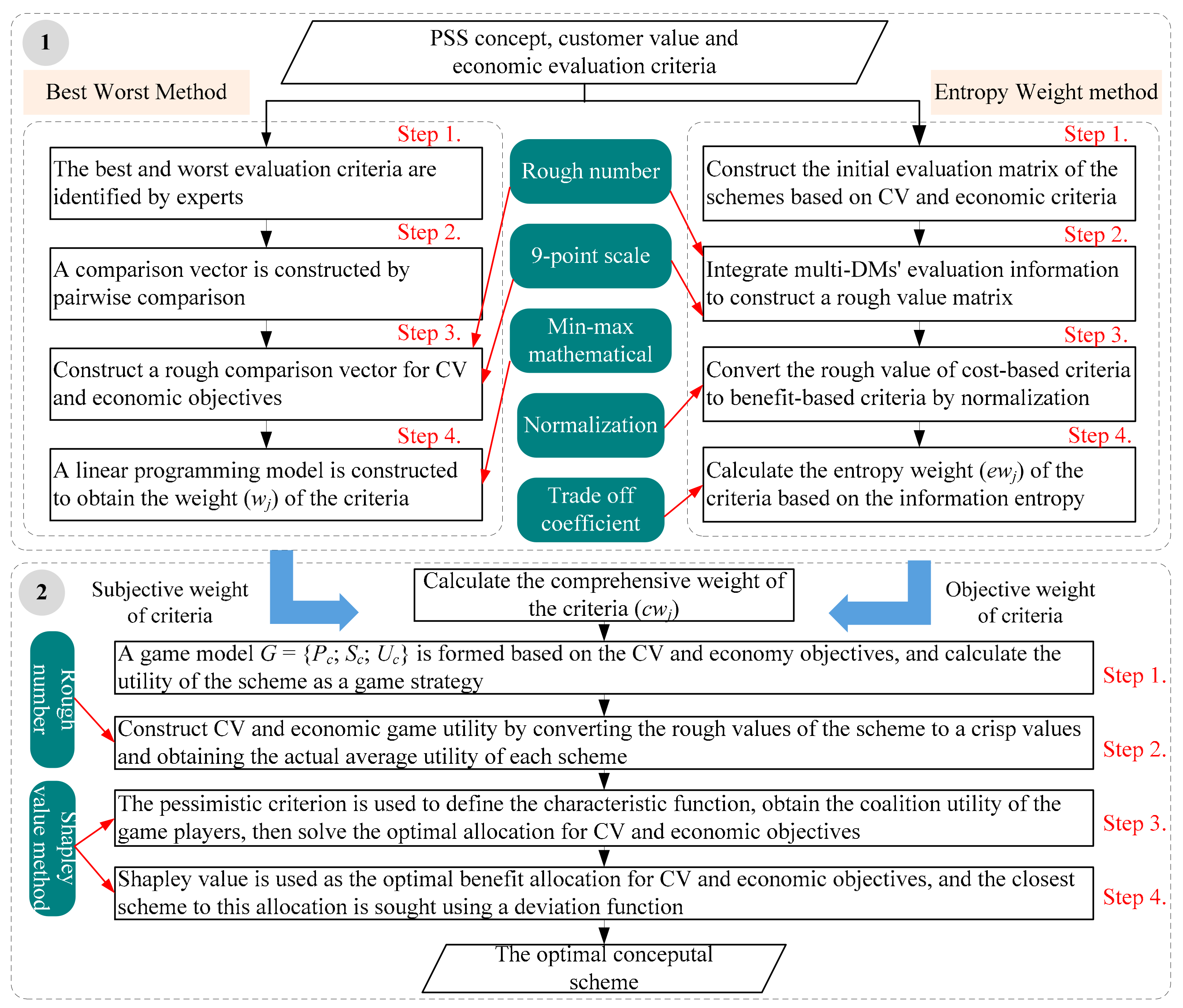
3.2. Calculation of Evaluation Criteria Weights Based on Rough BWM and Entropy Weight Method

In this section, the rough BWM and EWM methods are adopted simultaneously to compute the comprehensive weights of the CV and economic criteria. This approach circumvents the weakness of objective weight calculations (i.e., weights that do not consider DM preferences), and also reduces the uncertainty triggered by subjective preferences. In addition, the preference evaluation for criteria is evaluated by the DM using the so-called 9-point scale [34,44], which is defined as follows: 1, very low (VL); 3, low (L); 5, moderate (M); 7, high (H); 9, very high (VH); and 2, 4, 6, 8, intermediate values between the two adjacent judgments.

3.2.1. Calculation of Subjective Weights of Evaluation Criteria Using Rough BWM

Step 1. Let the set of CV evaluation criteria be {a₁, a₂, …, a_n}. The importance of each criterion is assessed via expert questionnaires [45], and the results of this assessment are adopted to identify the best criterion c_B and worst criterion c_W.

Step 2. Based on the 9-point scale, by determining the preference of the optimal criterion over other criterions, a best-to-others vector H^k_B = (h^k_B1, h^k_B2, …, h^k_Bn) is constructed. Similarly, the preference of other criteria for the worst criterion is evaluated, and an others-to-worst vector H^k_W = (h^k_1W, h^k_2W, …, h^k_nW) is constructed, where h^k_Wj represents the preference of DM k (1 ≤ k ≤ m) for other criteria j (1 ≤ j≤ n) compared to the worst criterion.

Step 3. Rough comparison vectors are constructed for all of the DMs [10,38]. Suppose that R^k_B1 = {h¹_B1, h²_B1 …, h^m_B1}, where any preference assessment relative to Criterion 1 is h_p ∈ h^k_B1, $\forall$X ∈ R^k_B1. The lower ($\underset{¯}{Apr}\left(h_p\right)$) and upper ($\overline{Apr}\left(h_p\right)$) approximations can then be defined as:

$$\begin{array}{l}\underset{¯}{Apr}(h_p)={\displaystyle \cup \{X\in R^k{{}_B}_1/R^k{{}_B}_1(X)\le h_p\}}\\ \overline{Apr}(h_p)={\displaystyle \cup \{X\in R^k{{}_B}_1/R^k{{}_B}_1(X)\ge h_p\}}\end{array}$$

(1)

Then, based on Equation (2), the rough number RN(h_p) is defined by its lower limit ($\underset{¯}{Lim}\left(h_p\right)$) and the upper limit ($\overline{Lim}\left(h_p\right)$), respectively.

$$\begin{array}{l}\underset{¯}{Lim}(h_p)=\frac{1}{Q_L}{\displaystyle \sum R_{Bi}(X)|Y\in \underset{¯}{Apr}(h_p)}\\ \overline{Lim}(h_p)=\frac{1}{Q_U}{\displaystyle \sum R_{Bi}(X)|Y\in \overline{Apr}(h_p)}\\ RN(h_p)=[\underset{¯}{Lim}(h_p),\overline{Lim}(h_p)]\end{array}$$

(2)

Equations (1) and (2) are used to construct rough comparison vectors, RN(h_Bj) and RN(h_jW), for criterion j, as expressed in Equation (3).

$$\begin{array}{l}RN(h_{Bj})=\{[\underset{¯}{h_{Bj}^1},\overline{h_{Bj}^1}],[\underset{¯}{h_{Bj}^2},\overline{h_{Bj}^2}],\cdots ,[\underset{¯}{h_{Bj}^m},\overline{h_{Bj}^m}]\}\\ RN(h_{jW})=\{[\underset{¯}{h_{jW}^1},\overline{h_{jW}^1}],[\underset{¯}{h_{jW}^2},\overline{h_{jW}^2}],\cdots ,[\underset{¯}{h_{jW}^m},\overline{h_{jW}^m}]\}\end{array}$$

(3)

Subsequently, the averages of the rough series can be expressed as rough numbers of the comparison vectors. The rough numbers, $\overline{RN}$(h_Bj) and $\overline{RN}$(h_jW), defined by Equation (4), can be transformed as follows: $\overline{RN}$(h_Bj) = {[$\underset{¯}{h_{B1}}$,$\overline{h_{B1}}$], [$\underset{¯}{h_{B2}}$,$\overline{h_{B2}}$], …, [$\underset{¯}{h_{Bn}}$,$\overline{h_{Bn}}$]}, $\overline{RN}$(h_jW) = {[$\underset{¯}{h_{1W}}$,$\overline{h_{1W}}$], [$\underset{¯}{h_{2W}}$,$\overline{h_{2W}}$], …, [$\underset{¯}{h_{nW}}$,$\overline{h_{nW}}$]}.

$$\begin{array}{l}\overline{RN}(h_{Bj})=[\underset{¯}{h_{Bj}},\overline{h_{Bj}}]=\frac{1}{m}{\displaystyle \sum _{k=1}^m[\underset{¯}{h_{Bj}^k},\overline{h_{Bj}^k}]}\\ \overline{RN}(h_{jW})=[\underset{¯}{h_{jW}},\overline{h_{jW}}]=\frac{1}{m}{\displaystyle \sum _{k=1}^m[\underset{¯}{h_{jW}^k},\overline{h_{jW}^k}]}\end{array}$$

(4)

where $\underset{¯}{h_{Bj}^k}$ and $\overline{h_{Bj}^k}$ represent the upper and lower boundaries of the rough number $\overline{RN}$(h_Bj), respectively, while $\underset{¯}{h_{jW}^k}$ and $\overline{h_{jW}^k}$ denote the upper and lower bounds of the rough number $\overline{RN}$(h_jW), respectively.

Step 4. A nonlinear min-max mathematical programming problem is constructed, as expressed in Equation (5). This is used to evaluate the rough weight of each criterion, RN(w_j). In addition, d([x],[y]) represents the degree of separation between the RN(x) and RN(y) rough sets [46], while [w_B] and [w_W] denote the weights of the best and worst criteria, respectively, as expressed in Equation (6).

$$\begin{array}{c}\min \underset{j}{\max }\left\{d(\frac{[w_B]}{[w_j]},[h_{Bj}]),d(\frac{[w_j]}{[w_W]},[h_{jW}])\right\};\hfill \\ \begin{array}{cc}\mathrm{s}.\mathrm{t}.& {\displaystyle \sum _{j=1}^n\underset{¯}{w_j}\le 1,\mathrm{for}\mathrm{all}j.}\hfill \\ & {\displaystyle \sum _{j=1}^n\overline{w_j}\ge 1},\mathrm{for}\mathrm{all}j.\hfill \\ & \overline{w_j}\ge \underset{¯}{w_j}\ge 0,\mathrm{for}\mathrm{all}j.\hfill \end{array}\hfill \end{array}$$

(5)

$$d([x],[y])=\sqrt{{(\underset{¯}{x}-\underset{¯}{y})}^2+{(\overline{x}-\overline{y})}^2}$$

(6)

Based on the rules of arithmetic operations with rough numbers and the characteristics of min-max programming problems [13], to obtain the optimal weights w_j = [w₁^*, w₂^*, …, w_n^*] and goals constraint ξ, an improved mathematical model was proposed by Rezaei [47], and the objective function was customized as follows:

$$\begin{array}{cc}\hfill \min & \zeta ;\hfill \\ \hfill \mathrm{s}.\mathrm{t}.& \left|\underset{¯}{w_B}-\overline{h_{Bj}}\overline{w_j}\right|\le \zeta ,\left|\overline{w_B}-\underset{¯}{h_{Bj}}\underset{¯}{w_j}\right|\le \zeta ,\mathrm{for}\mathrm{all}j.\hfill \\ & \left|\underset{¯}{w_j}-\overline{h_{jW}}\overline{w_W}\right|\le \zeta ,\left|\overline{w_j}-\underset{¯}{h_{jW}}\underset{¯}{w_W}\right|\le \zeta ,\mathrm{for}\mathrm{all}j.\hfill \\ & {\displaystyle \sum _{j=1}^n\underset{¯}{w_j}\le 1},{\displaystyle \sum _{j=1}^n\overline{w_j}\ge 1},\mathrm{for}\mathrm{all}j\hfill \\ & \overline{w_j}\ge \underset{¯}{w_j}\ge 0,\mathrm{for}\mathrm{all}j.\hfill \end{array}$$

(7)

where ξ denotes the goals constraint, and {[$\underset{¯}{w_1},\overline{w_1}$], [$\underset{¯}{w_2},\overline{w_2}$], …, [$\underset{¯}{w_n},\overline{w_n}$]} represent the optimal rough weights of criteria.

The Lingo18 software is used to solve the aforementioned linear programming problem, while Equation (8) is adopted to normalize the rough weights of the evaluation criteria and calculate their crisp weights (w_j, where w_j ∈ [0,1).

$$w_j=(1-\alpha )\underset{¯}{w_j}+\alpha \overline{w_j}$$

(8)

3.2.2. Calculation of Objective Weights of Evaluation Criteria Using the Entropy Weight Method

The entropy weight method describes the uncertainty of evaluation information in objectively analyzing the importance of the evaluation criteria [38,48]. To address biases in the subjective weighting solutions, an initial evaluation matrix for solution values is first constructed using the evaluation criteria. The EWM is then adopted to calculate the objective weight of each evaluation criterion.

Step 1. The CV evaluation criteria are first divided into quantitative and qualitative criteria. Then, the DM k evaluates the solution, and the evaluations of all DMs are gathered to construct the initial evaluation matrix IEM = (x_ij)_K×n, where 1 ≤ i ≤ K. In particular, qualitative criteria are evaluated using a 9-point scale. For quantitative criteria, each DM suggests an appropriate value according to his own perception and experience. For example, based on the criterion E1 in our case, the value judgments of CS₁ are assigned by four DMs, which are 1.75 (t), 1.80 (t), 1.50 (t), and 1.75 (t), respectively.

Step 2. Equations (1) and (2) are used to convert the evaluation data of the DMs into rough numbers and construct the rough value matrix (RVM) of the solutions, RVM = (x’_ij)_K×n. This matrix is adopted to compute objective evaluation data for the criteria weights.

Step 3. The RVM of the solutions in terms of CV criteria is first constructed, and then normalized using Equation (8). Subsequently, the rough values of the solutions in terms of cost criteria are converted into utility values to produce the normalized rough value matrix NRM = (f_ij)_K×n, which is adopted in subsequent dimensionless entropy weight and criteria effect calculations, as expressed in Equation (9).

$$r_{ij}=[r_{ij}^L,r_{ij}^U]=\left\{\begin{array}{l}\left[f_{ij}^L/\sqrt{{\displaystyle \sum _i{(f_{ij}^U)}^2}},h_{ij}^U/\sqrt{{\displaystyle \sum _i{(f_{ij}^L)}^2}}\right],j\in \mathrm{benefit}\mathrm{criterion}\\ \left[\left(1/f_{ij}^U\right)/\sqrt{{\displaystyle \sum _i{(1/f_{ij}^L)}^2}},\left(1/f_{ij}^L\right)/\sqrt{{\displaystyle \sum _i{(1/f_{ij}^U)}^2}}\right],j\in \mathrm{cost}\mathrm{criterion}\end{array}\right.$$

(9)

where f_ij^L and f_ij^U denote the lower and upper bounds of the rough number of criteria j in solution i, respectively.

Step 4. The information entropy ej of each evaluation criterion is calculated based on the normalized RVM. e_j represents a measure of the uncertainty of the solution values for each criterion j; the higher the value of e_j, the more consistent the data for an evaluation criterion, and the lower its weight. The formulas for calculating e_j are expressed in Equations (10) and (11):

$$e_j=\lambda (-\frac{1}{\ln K}{\displaystyle \sum _{i=1}^K{\mathrm{g}}_{ij}\ln g_{ij}})+(1-\lambda )(-\frac{1}{\ln K}{\displaystyle \sum _{i=1}^K{z}_{ij}\ln z_{ij}})$$

(10)

$${\mathrm{g}}_{ij}=\frac{\left(r_{ij}^L+r_{ij}^U\right)/2}{{\displaystyle \sum _{i=1}^K\left(r_{ij}^L+r_{ij}^U\right)/2}},z_{ij}=\frac{1-\left(r_{ij}^U-r_{ij}^L\right)}{K-{\displaystyle \sum _{i=1}^K\left(r_{ij}^U-r_{ij}^L\right)}}$$

(11)

where λ (0 < λ < 1) is the balancing coefficient for the median of the rough number and uncertainty of DM evaluations. In this study, λ was set to 0.5 in all e_j calculations.

Finally, Equation (12) is adopted to compute the entropy weight of each evaluation criterion using their information entropy, thus generating their objective weights.

$$e{w}_j=\left(1-e_j\right)/{\displaystyle \sum _{j=1}^l\left(1-e_j\right)}$$

(12)

Based on Equation (13), the normalized comprehensive weight function cw_j is constructed by integrating the subjective weight and objective entropy weight of each criterion in the aforementioned Section 3.2.1 and Section 3.2.2, and to ensure the stability of the ranking results of schemes.

$$c{w}_j=w_j\ast e{w}_j/{\displaystyle \sum _{j=1}^l\left(w_j\ast e{w}_j\right)}$$

(13)

3.3. Decision of the Optimal Solution Based on the Coalitional Game Model

Within the context of this study, the coalitional game model is a multi-objective cooperative game model that is used to analyze design preferences and internal relationships in CV and economic objectives. In this section, the coalitional game model will be used to analyze the coalitional utility of CV and economic objectives in different solutions. The Shapley value will then be adopted to obtain a fair allocation of utilities, to ensure that none of the players (objectives) will try to leave the coalition. Furthermore, the Shapley value of each objective is a fair payoff, which considers the interactions between all objectives in calculating the optimal payoff that maximizes coalitional utility. The Shapley values were obtained via the following procedure:

Step 1. Construction of the coalition game: Firstly, one must define the players, strategies, and utility of the coalition game model. The model is expressed as G = {P_c; S_c; U_c}, c ∈ P, E, while the CV and economic objectives are projected as players P_p and P_E, respectively. The strategy of P_p is S_p(CS_i) = {P₁(CS_i), …, P_M(CS_i)}, where M denotes the number of CV criteria, respectively. Similarly, the strategy of P_E is S_E(CS_i) = {P₁(CS_i), …, P_N(CS_i)}, where N denotes the number of economic criteria. Because each conceptual solution corresponds to the strategy sets of a pair of players, S = (S_P(CS_i), S_E(CS_i)), if one selects some strategy set such as CS_i, the player utilities are U_P(S_P(CS_i), S_E(CS_i)), and U_E(S_P(CS_i), S_E(CS_i)). Therefore, once a strategy has been determined for one player, the strategy of the other player is also determined. However, because the solution values of P_P and P_E in each evaluation criterion are different, any change in the strategy of P_p will inevitably affect the designed expectation of P_E, thereby changing the overall designed expectation of the solution. The conflict of interest between P_p and P_E must be balanced by selecting the strategy set that best satisfies the design expectations of both players, i.e., the optimal conceptual solution.

Step 2. Calculation of player utilities: Given that each strategy set (S_P(CS_i), S_E(CS_i)) corresponds to a conceptual solution, the player utilities reflect the expected value of each solution for a given strategy. Because each solution represents an attempt by the designer to balance the design requirements of the PSS, the evaluations of the solutions will exhibit conflicts or dependencies with each other, and the utility of one player will inevitably influence that of the other. The objective of the coalitional game is to determine the optimal allocation of utilities to CV and economic objectives, despite their mutual antagonism, to maximize the overall utility of the solution. After the strategy (CS_i) has been determined, it is necessary to consider the effects of the evaluation criteria (which have different weights) on player utility under the selected strategy set, and then objectively compute the utility of each player. First, the criteria weights (Equation (8)) are adopted to transform the solution’s normalized rough values in CV and economic objectives into crisp values r’_ij (α = 0.5). The weights are then applied to obtain the actual utilities of the players. To ensure that the utilities are expressed in a consistent, comparable and intuitive manner, the actual utilities of each player are averaged by their number of criteria. Finally, the relative average of all criteria relative to the average utility is considered the utility of the CV and economic objectives, as expressed in Equations (14) and (15).

$$ave\left(J_{j_c}\right)=\frac{1}{K}{\displaystyle \sum _{i=1}^{K}c{w}_{j_c}{r^{\prime }}_{j_c}(C{S}_i)},c\in \mathrm{P},\mathrm{E}$$

(14)

$$\begin{array}{l}{U}_{\mathrm{P}}\left(S_P(C{S}_i),S_E(C{S}_i)\right)=\frac{1}{M}\times {\displaystyle \sum _{j_{\mathrm{p}}=1}^M\frac{c{w}_{j_{\mathrm{p}}}{r^{\prime }}_{j_{\mathrm{p}}}(C{S}_i)}{ave\left(J_{j_{\mathrm{p}}}\right)}}\\ U_{\mathrm{E}}\left(S_P(C{S}_i),S_E(C{S}_i)\right)=\frac{1}{N}\times {\displaystyle \sum _{j_{\mathrm{E}}=1}^N\frac{c{w}_{j_{\mathrm{E}}}{r^{\prime }}_{j_{\mathrm{E}}}(C{S}_i)}{ave\left(J_{j_{\mathrm{E}}}\right)}}\end{array}$$

(15)

where ave(J_i) represents the average of all solution values in the criterion j, j_p and j_E denote the CV and economic objective, while r’_j(CS_i) is the crisp value of the criterion j in solution i.

Based on the utility function, the normalized rough values of each solution are adopted to obtain the CV and economic utilities of the various conceptual solutions. These utilities are then used to construct the utility matrix presented in

Table 4. Game utility matrix of scheme under each strategy combination.

Game Utility	Conceptual Scheme
	CS1	CS2	...	CSi
UP(SP, SE)	UP(SP(CS1), SE(CS1))	UP(SP(CS2), SE(CS2))	...	UP(SP(CSi), SE(CSi))
UE(SP, SE)	UE(SP(CS1), SE(CS1))	UE(SP(CS2), SE(CS2))	...	UE(SP(CSi), SE(CSi))

.

Step 3. Finding the optimal allocation of utilities: in a coalitional game, the players cooperate to maximize the utility of the coalition and their personal utility, as well as obtain a practical allocation of utilities (i.e., Shapley values). In the current context, the CV and economic objectives form a coalition N that attempts to maximize coalitional utility, where N = {P, E}. Three possible non-empty coalitions c exist: {P}, {E}, and {P, E}. To ensure that all players gain utility by cooperating with each other, instead of abandoning the coalition to form single coalitions (such as {P} or {E}), a pessimistic standard [25,49] was adapted to define the characteristic function that calculates the coalitional utility v({c}) of each player, as expressed in Equation (16). This approach ensures that coalitional utility is maximized if the players cooperate with each other, regardless of the strategy adopted by the coalition {c}.

$${\mathrm{a}}^v\left(\left\{c\right\}\right)=\min \underset{1\le i\le K}{\max }{U}_c\left(S_P(C{S}_i),S_E(C{S}_i)\right)$$

(16)

where c represents the players P and E.

The coalition {P, E}, which exists if the players are cooperating, has the characteristic function v({P, E}) = min{U_P + U_E}. Therefore, coalitional utility is maximized if the CV and economic players (P and E) cooperate with each other. This also implies that the coalition will still maximize the utility of each player despite their conflicting interests. The Shapley value is defined as φ(v) = (φ₁(v), φ₂(v), ..., φ_L(v)), and it is the optimal allocation of player utilities that will optimize the overall utility of the coalition. Because L is 2, φ(v) = (φ_P(v), φ_E(v)). In other words, the Shapley value balances the interests of the solution’s CV and economic objectives to provide the optimal allocation of utilities that maximizes coalitional and player utility in a competitive environment, as expressed in Equation (17). In addition, the Shapley value can be regarded as the expectation of each player’s utility in the overall coalition utility, thereby reflecting the importance degree of different players on the overall interest. The Shapley value is proportional to the contribution of a player to the designed value of the solution, as well as the influence of the player on the coalition’s overall utility.

$${\varphi }_c\left(v\right)={\displaystyle \sum _{S:c\notin S}\frac{\left|S\right|!\left(d-1-\left|S\right|\right)!}{d!}\times \left[v\left(S\cup \left\{c\right\}\right)-v\left(S\right)\right]}$$

(17)

where S is an arbitrary subset of coalition N that does not contain c, |S| is the number of players included in S, v = (S∪{c}) represents the coalition utility when S and the game player c cooperate, and d represents the number of players.

Step 4. Ranking solutions based on their Shapley values: Equation (18) is adopted to compute the optimal expected ratio of the players, (φ_P(v), φ_E(v)). The deviation function [50] is then used to compute the deviation of all solutions from this ratio. The solution with the smallest deviation is the design that maximizes the overall utility of the PSS; hence, it is the optimal solution. φ_P(v) and φ_E(v) represent the optimal balance between CV and economic objectives, respectively, and they ensure that the CV requirements will be satisfied with minimal losses in economic value. This will provide a fresh perspective for designers and enterprises, as it was impossible to evaluate the product-service value and cost during the early design phase. Moreover, the relative importance between the intrinsic service value and economic objectives of the scheme can be mined without auxiliary functions or parameters because the Shapley values were computed from the evaluation data of the initial solutions. Hence, this approach improves the objectivity of the decision.

$$D\left(C{S}_i\right)=\sqrt{{\left(U_P\left(C{S}_i\right)-{\varphi }_P\left(v\right)\right)}^2+{\left(U_E\left(C{S}_i\right)-{\varphi }_E\left(v\right)\right)}^2}$$

(18)

where U_E(Sch_j) and U_T(Sch_j) are the economic and technical utilities of solution j, D(CS_i) represents the deviation of solution i from the optimal distribution of utilities, and φ(v) = (φ_P(v), φ_E(v)).

4. Case Study

Owing to the rapid growth of small warehouse logistics, electric forklift buyers have become increasingly demanding in terms of their service requirements. For example, electric forklifts are now required to support online purchasing, online maintenance, and delayed scrapping, and this has intensified the competitiveness amongst forklift manufacturers [51,52]. To obtain a warehouse logistics solution that satisfies all CV and economic objectives in the initial design phase, forklift manufacturers must evaluate the CV and economic value of their warehouse logistics solutions within the design phase, and then select an optimal conceptual solution. Therefore, a case study of electric forklift PSS concept design is employed to verify the proposed decision model.

4.1. Determination of Evaluation Criteria for CV and Economic Value in the Electric Forklift PSS

The overall function of an electric forklift is to move goods using electrical power. According to its energy, material, and information flows, this function can be further decomposed into moving goods, turning wheels, increasing height, braking, changing directions, and operating the vehicle. The principal solutions that satisfy the aforementioned functions were obtained by searching through the product knowledgebase; these solutions were then adopted to construct the morphological matrix of an electric forklift, as presented in

Table 5. Morphology matrix of electric forklifts.

Sub-Function		Principle Solution
		1	2	3	4
A	Carrying the goods	Secondary gantry	Secondary fully free gantry	Three-stage fully free gantry
B	Driving wheel	Mechanical drive	Fluid drive	Hydraulic drive
C	Convert electricity	AC MOTOR	DC MOTOR
D	Hoisting height	Chain wheel	Belt wheel	Hydraulic	Gear
E	Brake mode	Manual hydraulic	Electro hydraulic
F	Steering mode	Mechanical manual steering	Manual hydraulic steering	Electro hydraulic steering
G	Operating handle	Vertical handle	Side handling handle

.

Six research students from our group were asked to screen the principal solutions by using a Pugh table to qualitatively ascertain the initial principal solution combinations. Accordingly, the principal solutions that were clearly impractical were eliminated (the screening process will not be described in further detail, and interested readers can refer to [44]). Finally, a total of six candidate concept schemes were selected, with the names CS1 (A1B3C1D3E1F2G1); CS2 (A1B3C1D1E1F2G2), CS3 (A2B3C1D3E2F3G1), CS4 (A1B1C1D3E1F1G1), CS5 (A3B3C1D3E2F3G1), and CS6 (A1B3C1D3E2F3G2), respectively. In addition, SM and SC in Figure 2 denote the service modules in the electric forklift PSS and the corresponding sub-items, respectively, as shown in

Table A1. Service module of the electric storage and handling system of electric forklift PSS.

Items	Service Module	Sub-Items	Service Components
SM1	Guidance and training	SC1.1	Performance parameter library
		SC1.2	Equipment selection specification
		SC1.3	Operation specification
		SC1.4	System price composition
		SC1.5	Instructor
		SC1.6	Training processes and specifications
		SC1.7	Remote communication platform
		SC1.8	Customer experience platform
		SC1.9	Typical problem processing database
SM2	Spare parts supply	SC2.1	Spare parts sales platform
		SC2.2	Spare parts performance database
		SC2.3	Supply of spare parts information base
SM3	Routine maintenance	SC3.1	Maintenance knowledge database
		SC3.2	Maintenance record information database
		SC3.3	Maintenance price composition
		SC3.4	Maintenance tools
		SC3.5	Maintenance staff
		SC3.6	Maintenance flow and specifications
SM4	Troubleshooting	SC4.1	Equipment troubleshooting device
		SC4.2	Equipment troubleshooting platform
		SC4.3	Fault information knowledge base
		SC4.4	Troubleshooting staff
		SC4.5	Troubleshooting tools
SM5	Delivery distribution	SC5.1	System sales platform
		SC5.2	Logistics and distribution system
		SC5.3	Financial payment system
SM6	Field service	SC6.1	Field service appointment platform
		SC6.2	Field service price composition
		SC6.3	Field service knowledge base
		SC6.4	Field service staff
		SC6.5	Field service flow and specifications
		SC6.6	Service tools
SM7	Factory service	SC7.1	Factory service appointment platform
		SC7.2	Factory service knowledge base
		SC7.3	Factory service staff
		SC7.4	Factory service equipment
		SC7.5	Factory service progress information exchange platform
SM8	Scrap recycling	SC8.1	Recycling knowledge database
		SC8.2	Recycling price composition
		SC8.3	Recycling tools
		SC8.4	Recycling staff
		SC8.5	Recycling process and specifications

.

The technical, operational, and design characteristics of warehouse logistics systems were used to determine their economic requirements. Accordingly, eight evaluation criteria were formed, which include E1 (rated lifting capacity), E2 (maximum driving speed), E3 (maximum lifting height), E4 (motor power), E5 (production cost), E6 (maintenance cost), E7 (safety), and E8 (forklift weight). The specific definitions and categories of these criteria are presented in

Table 6. Description of evaluation criteria in the economic objective of warehouse logistics system.

Label	Criterion	Description	Category
E1	Rated lifting capacity	The maximum mass allowed for forklift loads when the center of gravity is within the standard load center distance of the forklift truck	Benefit
E2	Maximum driving speed	The maximum steady speed of the forklift truck when the fork carries the rated load at maximum speed	Benefit
E3	Maximum lifting height	The height that the forklift can lift when it is on level ground and the fork carries the rated lifting weight	Benefit
E4	Motor power	The maximum power that the motor can run normally when the forklift is on the level ground and running stably after starting	Benefit
E5	Production cost	The total cost of the forklift after design, processing and assembly, including materials, supplies, research and development, etc	Cost
E6	Maintenance costs	The expenses for regular inspection, maintenance and replacement of vulnerable parts of the forklift	Cost
E7	Safety	The reliability of forklift design and the ability to protect the driver and cargo during operation and operation	Benefit
E8	Forklift weight	The total weight of all parts of a forklift truck when it is not loaded	Cost

. Here, it should be noted that economic value in the context of CV pertains to the customer’s user experience or psychological expectations, while cost-related economic objectives are related to product costs due to design-related activities such as structural optimization, manufacturing, and assembly.

4.2. Calculation of Criteria Weights Integrating Rough BWM and Entropy Weight Method

4.2.1. Calculation of Subjective Weights of CV and Economic Criteria for Warehouse Logistics System

Step 1. Consistent with previous studies [53], four experts were invited to determine the best and worst criteria. The selected experts possess skills and experience in the design and development of warehouse logistics PSSs, and they include one forklift designer, one service engineer, one manufacturing engineer, and one PSS researcher. The best and worst CV criteria were P1 and P5, while the best and worst economic criteria were E7 and E8, respectively.

Step 2. The four DMs were asked to compare each criterion to c_B and c_W on a 9-point scale. Then, the best-to-others vector and the others-to-worst vector were obtained through comparison between criteria, as shown in Equations (19) and (20). Among them, h^k_WW = 1 and h^k_BB = 1.

$$\begin{array}{c}\mathrm{PSS}\mathrm{criteria}\text{:}\begin{array}{cccccccccc}1& 2& 3& 4& 5& 6& 7& 8& 9& 10\end{array}\\ H_B^P=\begin{array}{c}{\mathrm{DM}}_1\\ {\mathrm{DM}}_2\\ {\mathrm{DM}}_3\\ {\mathrm{DM}}_4\end{array}\left[\begin{array}{cccccccccc}1& 2& 6& 6& 9& 6& 8& 4& 2& 4\\ 1& 3& 3& 6& 9& 5& 5& 6& 2& 6\\ 1& 2& 2& 7& 9& 2& 5& 2& 5& 6\\ 1& 2& 3& 6& 9& 5& 3& 3& 5& 3\end{array}\right],\end{array}\begin{array}{c}\begin{array}{cccccccccc}1& 2& 3& 4& 5& 6& 7& 8& 9& 10\end{array}\\ H_W^P=\left[\begin{array}{cccccccccc}9& 6& 6& 3& 1& 4& 4& 3& 7& 3\\ 9& 6& 6& 3& 1& 7& 4& 7& 4& 3\\ 9& 4& 7& 6& 1& 6& 3& 5& 4& 3\\ 9& 6& 6& 3& 1& 4& 6& 6& 4& 6\end{array}\right]\end{array}$$

(19)

$$\begin{array}{c}\mathrm{Economic}\mathrm{criteria}:\begin{array}{cccccccc}1& 2& 3& 4& 5& 6& 7& 8\end{array}\hfill \\ H_B^E=\begin{array}{c}{\mathrm{DM}}_1\\ {\mathrm{DM}}_2\\ {\mathrm{DM}}_3\\ {\mathrm{DM}}_4\end{array}\left[\begin{array}{cccccccc}3& 4& 1& 4& 3& 4& 1& 9\\ 3& 1& 2& 5& 2& 8& 1& 9\\ 1& 5& 1& 3& 3& 4& 1& 9\\ 1& 4& 2& 2& 4& 2& 1& 9\end{array}\right],\end{array}\begin{array}{c}\begin{array}{cccccccc}1& 2& 3& 4& 5& 6& 7& 8\end{array}\\ H_W^E=\left[\begin{array}{cccccccc}6& 9& 7& 4& 7& 1& 9& 1\\ 8& 4& 8& 6& 6& 5& 9& 1\\ 7& 4& 6& 3& 6& 9& 9& 1\\ 9& 5& 7& 7& 5& 7& 9& 1\end{array}\right]\end{array}$$

(20)

Step 3. The rough comparison vector for the CV and economic objectives were calculated by Equations (1) and (2). Taking the results of the best criterion P1 to P2 as an example, the result was {2,3,2,2}, RN(h^P_B2) = {[2,2.75], [2.33,3.5], [2,2.75], [2.75,4]}, and the average rough set was $\overline{RN}$(h^P_B2) = [(2 + 2.333 + 2 + 2.75)/4, (2.75 + 3.5 + 2.75 + 4)/4] = [2.271,3.250]. Then, the rough sets of other evaluation criteria were integrated to construct the rough comparison vector, as shown in

Table 7. The results of $\overline{RN}$(h_Bj), $\overline{RN}$(h_jW) and weight w_j of the criteria in CV and economic objective.

(a) The Subjective Weights of Criteria in the CV Objective
Criteria	$\overline{\mathit{R}\mathit{N}}\left({{\mathit{h}}^{\mathit{P}}}_{\mathit{Bj}}\right)$	$\overline{\mathit{R}\mathit{N}}\left({{\mathit{h}}^{\mathit{P}}}_{\mathit{jW}}\right)$	RN(wPj)	wPj
P1	[1,1]	[9,9]	[0.289,0.289]	0.266
P2	[2.271,3.250]	[5.104,6.354]	[0.100,0.100]	0.092
P3	[2.708,4.375]	[6.271,7.250]	[0.123,0.146]	0.124
P4	[6.271,7.250]	[3.333,4.750]	[0.060,0.060]	0.055
P5	[9,9]	[1,1]	[0.025,0.025]	0.023
P6	[3.625,5.292]	[4.479,6.000]	[0.091,0.100]	0.088
P7	[4.229,6.313]	[3.646,4.896]	[0.063,0.073]	0.062
P8	[2.813,4.771]	[4.229,6.188]	[0.096,0.122]	0.100
P9	[1.875,3.000]	[4.333,5.750]	[0.085,0.171]	0.118
P10	[4.000,5.521]	[3.479,5.000]	[0.066,0.093]	0.073
(b) The Subjective Weights of Criteria in the Economic Objective
Criteria	RN(hEBj)	RN(hEjW)	RN(wEj)	wEj
E1	[1.333,2.500]	[6.750,8.250]	[0.056,0.061]	0.059
E2	[2.625,4.292]	[4.458,6.750]	[0.186,0.186]	0.188
E3	[1.250,1.750]	[6.583,7.417]	[0.225,0.225]	0.228
E4	[2.750,4.250]	[3.958,6.042]	[0.146,0.165]	0.157
E5	[2.583,3.417]	[5.583,6.417]	[0.020,0.020]	0.020
E6	[3.292,5.792]	[3.458,7.375]	[0.050,0.050]	0.051
E7	[1,1]	[9,9]	[0.278,0.278]	0.281
E8	[9,9]	[1,1]	[0.016,0.016]	0.016

.

Step 4. By constructing the rough comparison vector, a programming problem was constructed according to Equations (6) and (7). LINGO 16.0 was used to solve this problem, and the rough weight vectors for criteria are described in

Table 8. Initial evaluation matrix of the electric forklift PSS concept (taking the CS₁ as an example).

(a) Scheme Value Assessment of Criteria in the CV Objective
Evaluation Criteria	Evaluation Value Assigned by Four DMs
	DM1	DM2	DM3	DM4
P1	6	6	2	8
P2	6	3	4	3
P3	6	7	4	5
P4	4	4	3	3
P5	5	6	4	6
P6	5	8	4	6
P7	5	7	4	4
P8	6	8	6	4
P9	6	5	6	6
P10	6	4	4	8
(b) Scheme Value Assessment of Criteria in the Economic Objective
Evaluation Criteria	Evaluation Value Assigned by Four DMs
	DM1	DM2	DM3	DM4
E1 (t)	1.75	1.80	1.50	1.75
E2 (km/h)	13	13	16	13
E3 (mm)	3500	4000	4000	3000
E4 (kw)	4	6	6	4
E5 (¥)	14,400	9600	12,000	12,500
E6	6	2	5	2
E7	6	7	7	6
E8 (t)	3.75	3.5	3.5	3.5

. Next, the crisp weight was obtained by using Equation (8).

4.2.2. Calculation of Objective Weights of CV and Economic Criteria for the Electric Forklifts PSS

Step 1. The four DMs evaluated the CV of the PSS solutions according to the aforementioned evaluation criteria. Qualitative criteria were assessed by a 9-point scale, where a score of 9 represents the value of the solution that is most consistent with the criteria, and a score of 1 indicates that the value of the solution is the least consistent. In addition, considering the limitation of paper length, this study took the CS₁ as an example to construct the initial evaluation matrix of electric forklift, as shown in Table 8. Additionally, other evaluation matrixes were used for the remaining schemes in Appendix A, as shown in

Table A2. Initial evaluation matrix of the electric forklift PSS concept (taking the CS2 as an example).

(a) Scheme Value Assessment of Evaluation Criteria on the PSS Design
Evaluation Criteria	Evaluation Value Assigned by Four DMs
	DM1	DM2	DM3	DM4
P1	4	3	3	4
P2	6	4	4	3
P3	7	8	4	4
P4	5	5	4	3
P5	6	4	4	5
P6	4	6	3	5
P7	4	6	4	6
P8	5	4	6	3
P9	5	6	6	8
P10	4	4	4	6
(b) Scheme Value Assessment of Evaluation Criteria on the Economy
Evaluation Criteria	Evaluation Value Assigned by Four DMs
	DM1	DM2	DM3	DM4
E1 (t)	2.25	2.75	1.5	2.25
E2 (km/h)	16	20	16	13
E3 (mm)	3000	4000	4000	4000
E4 (kw)	6	8	6	4
E5 (yuan)	14,400	12,000	12,000	14,400
E6	6	6	7	5
E7	4	6	7	5
E8 (t)	4.5	5	3	4

,

Table A3. Initial evaluation matrix of the electric forklift PSS concept (taking the CS3 as an example).

(a) Scheme Value Assessment of Evaluation Criteria on the PSS Design
Evaluation Criteria	Evaluation Value Assigned by Four DMs
	DM1	DM2	DM3	DM4
P1	7	4	6	6
P2	7	6	6	6
P3	6	5	6	5
P4	6	5	6	7
P5	5	4	4	5
P6	7	6	3	6
P7	7	6	5	6
P8	7	8	6	5
P9	7	7	4	7
P10	7	6	6	7
(b) Scheme Value Assessment of Evaluation Criteria on the Economy
Evaluation Criteria	Evaluation Value Assigned by Four DMs
	DM1	DM2	DM3	DM4
E1 (t)	2.75	2.75	3	2.25
E2 (km/h)	13	13	20	13
E3 (mm)	3000	3500	3000	3000
E4 (kw)	6	7	8	6
E5 (yuan)	16,800	10,000	14,400	12,000
E6	6	7	6	4
E7	7	8	5	6
E8 (t)	5	5	6	4

,

Table A4. Initial evaluation matrix of the electric forklift PSS concept (taking the CS4 as an example).

(a) Scheme Value Assessment of Evaluation Criteria on the PSS Design
Evaluation Criteria	Evaluation Value Assigned by Four DMs
	DM1	DM2	DM3	DM4
P1	5	8	8	3
P2	4	3	3	2
P3	7	4	3	2
P4	5	7	3	5
P5	6	3	4	4
P6	5	6	6	6
P7	6	2	3	5
P8	5	4	6	6
P9	5	7	8	7
P10	5	3	3	4
(b) Scheme Value Assessment of Evaluation Criteria on the Economy
Evaluation Criteria	Evaluation Value Assigned by Four DMs
	DM1	DM2	DM3	DM4
E1 (t)	1.75	1.5	1.75	2.75
E2 (km/h)	16	10	10	10
E3 (mm)	4000	4000	4500	3500
E4 (kw)	4	4	4	4
E5 (yuan)	12,000	14,400	10,000	9600
E6	5	4	4	3
E7	5	5	5	7
E8 (t)	3.5	2.5	3.5	5

,

Table A5. Initial evaluation matrix of the electric forklift PSS concept (taking the CS5 as an example).

(a) Scheme Value Assessment of Evaluation Criteria on the PSS Design
Evaluation Criteria	Evaluation Value Assigned by Four DMs
	DM1	DM2	DM3	DM4
P1	8	6	5	6
P2	8	8	6	6
P3	6	7	6	4
P4	7	5	7	6
P5	7	6	4	7
P6	8	8	5	8
P7	7	4	6	6
P8	8	3	6	7
P9	7	4	4	5
P10	8	9	6	9
(b) Scheme Value Assessment of Evaluation Criteria on the Economy
Evaluation Criteria	Evaluation Value Assigned by Four DMs
	DM1	DM2	DM3	DM4
E1 (t)	3	3.5	3	3
E2 (km/h)	13	20	20	20
E3 (mm)	4500	5000	5000	5000
E4 (kw)	7	9	8	8
E5 (yuan)	16,800	19,200	14,400	19,200
E6	7	7	7	6
E7	8	4	6	6
E8 (t)	5.5	6.5	6	6

and

Table A6. Initial evaluation matrix of the electric forklift PSS concept (taking the CS5 as an example).

(a) Scheme Value Assessment of Evaluation Criteria on the PSS Design
Evaluation Criteria	Evaluation Value Assigned by Four DMs
	DM1	DM2	DM3	DM4
P1	7	7	6	5
P2	7	9	8	6
P3	5	5	8	6
P4	6	6	8	5
P5	7	3	6	4
P6	7	4	6	7
P7	7	7	7	7
P8	7	7	7	8
P9	7	5	5	6
P10	7	6	8	5
(b) Scheme Value Assessment of Evaluation Criteria on the Economy
Evaluation Criteria	Evaluation Value Assigned by Four DMs
	DM1	DM2	DM3	DM4
E1 (t)	2.25	2.25	1.75	2.75
E2 (km/h)	13	20	16	16
E3 (mm)	4000	4000	4500	3000
E4 (kw)	6	9	9	7
E5 (yuan)	14,400	14,400	19,200	16,800
E6	6	3	8	5
E7	7	5	7	7
E8 (t)	4.5	4.5	3.5	5

.

Step 2. To provide objective information on the value of each solution, rough numbers were generated using the data in the initial evaluation matrix. Taking the sequence of the criterion E1 for CS₁ as an example, the sequence was [1.75, 1.80, 1.50, 1.75], $\underset{¯}{Lim}\left(1.75\right)$ = (1.75 + 1.5 + 1.75)/3 = 1.667, $\overline{Lim}\left(1.75\right)$ = (1.75 + 1.8 + 1.75)/3 = 1.767, $\underset{¯}{Lim}\left(1.8\right)$ = (1.75 + 1.8 + 1.5 + 1.75)/4 = 1.7, $\overline{Lim}\left(1.8\right)$ = (1.8)/1 = 1.8, $\underset{¯}{Lim}\left(1.5\right)$ = (1.5)/1 = 1.5, $\overline{Lim}\left(1.5\right)$ = (1.75 + 1.8 + 1.5 + 1.75)/4 = 1.7. Based on Equations (1) and (2), the rough value of CS1 with respect to the criterion E1 was calculated as RN(E¹₁) = RN(E⁴₁) = RN(1.75) = [1.667,1.767], RN(E²₁) = RN(1.8) = [1.7,1.8], RN(E³₁) = RN(1.5) = [1.5,1.7]. The average rough set was [(1.667 + 1.7 + 1.5 + 1.667)/4, (1.767 + 1.8 + 1.7 + 1.767)/4] = [1.633, 1.758]. The previous step was then repeated to obtain RVMs for the CV and economic objectives, as expressed in Equations (21) and (22).

$${\rm P}V{{\rm M}}_{\mathrm{P}}=\begin{array}{cc}& \begin{array}{cccccc}\hspace{1em}\hspace{1em}\hspace{1em}C{S}_1\hspace{1em}\hspace{1em}\hspace{1em}& C{S}_2\hspace{1em}\hspace{1em}\hspace{1em}\hspace{1em}& C{S}_3\hspace{1em}\hspace{1em}\hspace{1em}\hspace{1em}& C{S}_4\hspace{1em}\hspace{1em}\hspace{1em}& C{S}_5\hspace{1em}\hspace{1em}\hspace{1em}& C{S}_6\hspace{1em}\hspace{1em}\hspace{1em}\hspace{1em}\end{array}\\ \begin{array}{c}P1\\ P2\\ P3\\ P4\\ P5\\ P6\\ P7\\ P8\\ P9\\ P10\end{array}& \left[\begin{array}{cccccc}[4.208,6.708]& [3.250,3.750]& [5.104,6.354]& [4.750,7.250]& [5.583,6.833]& [5.625,6.667]\\ [3.363,4.775]& [3.563,4.896]& [6.063,6.438]& [2.583,3.417]& [6.500,7.500]& [6.750,8.250]\\ [4.750,6.250]& [4.688,6.750]& [5.250,5.750]& [2.875,5.292]& [5.104,6.354]& [5.333,6.750]\\ [3.250,3.750]& [4.250,4.750]& [5.583,6.417]& [4.167,5.833]& [5.750,6.729]& [5.646,6.368]\\ [5.250,5.750]& [4.271,5.250]& [4.250,4.750]& [3.646,4.896]& [5.250,6.667]& [3.958,6.042]\\ [4.813,6.771]& [3.750,5.250]& [4.625,6.292]& [5.563,5.938]& [6.688,7.813]& [5.250,6.667]\\ [4.333,5.750]& [4.500,5.500]& [5.583,6.417]& [2.958,5.042]& [5.104,6.354]& [7.000,7.000]\\ [5.167,6.833]& [3.750,5.250]& [6.000,7.250]& [4.750,5.729]& [4.708,7.125]& [7.063,7.438]\\ [5.563,5.938]& [5.646,6.896]& [5.688,6.813]& [6.104,7.354]& [4.333,5.750]& [5.271,6.250]\\ [4.542,6.500]& [4.125,4.875]& [6.250,6.750]& [3.208,4.250]& [7.250,8.667]& [5.750,7.250]\end{array}\right]\end{array}$$

(21)

$$RV{M}_{\mathrm{E}}=\begin{array}{cc}& \begin{array}{cccccc}\hspace{1em}C{S}_1\hspace{1em}\hspace{1em}\hspace{1em}\hspace{1em}& C{S}_2\hspace{1em}\hspace{1em}\hspace{1em}\hspace{1em}& C{S}_3\hspace{1em}\hspace{1em}\hspace{1em}\hspace{1em}& C{S}_4\hspace{1em}\hspace{1em}\hspace{1em}\hspace{1em}& C{S}_5\hspace{1em}\hspace{1em}\hspace{1em}\hspace{1em}& C{S}_6\hspace{1em}\hspace{1em}\hspace{1em}\end{array}\\ \begin{array}{c}E1\\ E2\\ E3\\ E4\\ E5\\ E6\\ E7\\ E8\end{array}& \left[\begin{array}{cccccc}[1.663,1.758]& [1.922,2.443]& [2.526,2.839]& [1.693,2.214]& [3.031,3.219]& [2.042,2.458]\\ [13.188,14.313]& [14.813,17.729]& [13.438,16.063]& [10.375,12.625]& [16.646,19.563]& [15.500,18.979]\\ [3375,3865]& [3563,3938]& [3031,3219]& [3792,4208]& [4781,4969]& [3552,4177]\\ [4.500,5.500]& [6.271,7.250]& [6.271,7.250]& [3.750,4.729]& [7.583,8.417]& [7.000,8.521]\\ [11181,13260]& [11192,13025]& [11608,15025]& [10358,12808]& [16200,18550]& [15050,17400]\\ [3.292,5.708]& [3.750,5.250]& [5.104,6.354]& [4.333,5.750]& [6.563,6.938]& [6.750,8.250]\\ [6.250,6.750]& [4.750,6.250]& [5.750,7.250]& [5.125,5.875]& [4.542,6.500]& [5.000,6.521]\\ [3.516,3.609]& [3.656,4.594]& [4.583,5.417]& [3.115,4.156]& [5.792,6.208]& [4.052,4.677]\end{array}\right]\end{array}$$

(22)

Step 3. The CV and economic RVMs of the PSSs were normalized using Equation (9). The solution values relative to P10, E5, E6, and E8 were then converted into utility values to obtain the normalized rough value matrices associated with the CV and economic value, NRM_p and NRM_E, as expressed in Equations (23) and (24).

$$NR{M}_{\mathrm{P}}=\begin{array}{cc}& \begin{array}{cccccc}\hspace{1em}C{S}_1\hspace{1em}\hspace{1em}\hspace{1em}& C{S}_2\hspace{1em}\hspace{1em}\hspace{1em}& C{S}_3\hspace{1em}\hspace{1em}\hspace{1em}& C{S}_4\hspace{1em}\hspace{1em}\hspace{1em}& C{S}_5\hspace{1em}\hspace{1em}\hspace{1em}& C{S}_6\hspace{1em}\hspace{1em}\hspace{1em}\end{array}\\ \begin{array}{c}P1\\ P2\\ P3\\ P4\\ P5\\ P6\\ P7\\ P8\\ P9\\ P10\end{array}& \left[\begin{array}{cccccc}[0.270,0.568]& [0.208,0.317]& [0.327,0.538]& [0.305,0.613]& [0.358,0.578]& [0.361,0.564]\\ [0.225,0.383]& [0.238,0.393]& [0.405,0.517]& [0.173,0.274]& [0.434,0.602]& [0.451,0.662]\\ [0.312,0.538]& [0.308,0.581]& [0.345,0.495]& [0.189,0.456]& [0.355,0.547]& [0.350,0.581]\\ [0.231,0.315]& [0.302,0.398]& [0.397,0.538]& [0.296,0.489]& [0.409,0.565]& [0.402,0.534]\\ [0.383,0.524]& [0.311,0.478]& [0.310,0.433]& [0.266,0.446]& [0.383,0.608]& [0.289,0.551]\\ [0.302,0.532]& [0.235,0.413]& [0.290,0.495]& [0.349,0.467]& [0.420,0.614]& [0.330,0.524]\\ [0.293,0.463]& [0.304,0.443]& [0.377,0.517]& [0.200,0.406]& [0.345,0.512]& [0.473,0.564]\\ [0.317,0.522]& [0.230,0.401]& [0.368,0.554]& [0.291,0.438]& [0.289,0.544]& [0.433,0.568]\\ [0.348,0.444]& [0.353,0.515]& [0.356,0.509]& [0.382,0.550]& [0.271,0.430]& [0.330,0.467]\\ [0.291,0.526]& [0.388,0.579]& [0.280,0.382]& [0.445,0.744]& [0.218,0.329]& [0.261,0.415]\end{array}\right]\end{array}$$

(23)

$$NR{M}_{\mathrm{E}}=\begin{array}{cc}& \begin{array}{cccccc}\hspace{1em}C{S}_1\hspace{1em}\hspace{1em}\hspace{1em}& C{S}_2\hspace{1em}\hspace{1em}\hspace{1em}& C{S}_3\hspace{1em}\hspace{1em}\hspace{1em}& C{S}_4\hspace{1em}\hspace{1em}\hspace{1em}& C{S}_5\hspace{1em}\hspace{1em}\hspace{1em}& C{S}_6\hspace{1em}\hspace{1em}\hspace{1em}\end{array}\\ \begin{array}{c}E1\\ E2\\ E3\\ E4\\ E5\\ E6\\ E7\\ E8\end{array}& \left[\begin{array}{cccccc}[0.282,0.323]& [0.310,0.451]& [0.408,0.524]& [0.273,0.409]& [0.489,0.594]& [0.330,0.454]\\ [0.322,0.413]& [0.361,0.512]& [0.328,0.464]& [0.253,0.365]& [0.406,0.565]& [0.378,0.548]\\ [0.336,0.424]& [0.355,0.432]& [0.302,0.353]& [0.378,0.462]& [0.477,0.545]& [0.354,0.458]\\ [0.259,0.371]& [0.361,0.489]& [0.361,0.489]& [0.216,0.319]& [0.437,0.568]& [0.403,0.575]\\ [0.373,0.531]& [0.379,0.531]& [0.329,0.512]& [0.386,0.574]& [0.266,0.367]& [0.284,0.395]\\ [0.320,0.766]& [0.348,0.672]& [0.287,0.494]& [0.317,0.582]& [0.263,0.384]& [0.221,0.373]\\ [0.390,0.523]& [0.297,0.484]& [0.359,0.562]& [0.320,0.455]& [0.284,0.504]& [0.312,0.505]\\ [0.440,0.530]& [0.345,0.510]& [0.293,0.407]& [0.382,0.599]& [0.256,0.322]& [0.339,0.460]\end{array}\right]\end{array}$$

(24)

Step 4. Based on the normalized rough value matrices (Equations (23) and (24)), Equations (10)–(12) were used to compute the objective weights of the CV and economic criteria, with λ = 0.5. The results are presented in

Table 9. Comprehensive weight of evaluation criteria with respect to CV and economic.

CV Criteria	ewj	wj	cwj	Economic Criteria	ewj	wj	cwj
P1	0.108	0.266	0.287	E1	0.154	0.059	0.097
P2	0.270	0.092	0.249	E2	0.086	0.188	0.172
P3	0.042	0.124	0.052	E3	0.069	0.228	0.167
P4	0.106	0.055	0.058	E4	0.180	0.157	0.301
P5	0.045	0.023	0.010	E5	0.092	0.020	0.020
P6	0.056	0.088	0.049	E6	0.262	0.051	0.142
P7	0.079	0.062	0.049	E7	0.026	0.281	0.078
P8	0.066	0.100	0.066	E8	0.132	0.016	0.023
P9	0.024	0.118	0.028
P10	0.205	0.073	0.150

.

4.2.3. Calculation of Comprehensive Weights of Evaluation Criteria

Equation (13) was used to calculate comprehensive criteria weights (cw_j) based on the subjective and objective criteria weights from steps (1) and (2). The obtained results are presented in Table 9. In the design of electric forklifts, the CV criteria that are most important for experts include reliability (P1), digital controlling and smartness (P2), and total cost for PSS (P10). The most important economic criteria are maximum driving speed (E2), maximum lifting height (E3), and maintenance cost (E6).

4.3. Determination of the Optimal Solution Based on the Coalitional Game Model

Step 1. The strategy sets of six conceptual solutions for warehouse logistics systems were obtained, which include (S_P(CS₁), S_E(CS₁))–(S_P(CS₆), S_E(CS₆)). The interactions between CV and economic objectives are illustrated in Figure 3, and it is shown that the criteria weights of each objective will affect utility. Hence, the criteria weights were considered in utility calculations.

Step 2. The normalized rough values of the warehouse logistics system solutions (Equations (23) and (24)) were converted into crisp values. Equations (14) and (15) were then adopted to calculate the utilities of the CV and economic objectives in each strategy set. The calculated utilities of the electric forklift solutions are presented in

Table 10. Game utility matrix of warehouse logistics system under each strategy combination.

Game Utility	Conceptual Scheme
	CS1	CS2	CS3	CS4	CS5	CS6
UP(SP, SE)	0.946	0.901	1.027	0.946	1.070	1.110
UE(SP, SE)	1.004	1.043	0.988	0.959	1.029	0.977

.

Step 3. Based on

Table 11. The sorting results of the scheme under different α values.

α value	Sorting Results	The Optimal Scheme	(UP, UE)	(φP(v), φE(v))
α = 0	CS4 > CS1 > CS2 > CS3 > CS5 > CS6	CS4	(0.898,0.940)	(0.895,0.944)
α = 0.1	CS4 > CS1 > CS2 > CS3 > CS5 > CS6	CS4	(0.910,0.945)	(0.902,0.953)
α = 0.3	CS4 > CS1 > CS2 > CS3 > CS5 > CS6	CS4	(0.930,0.952)	(0.914,0.968)
α = 0.5	CS1 > CS4 > CS2 > CS3 > CS5 > CS6	CS1	(0.946,1.004)	(0.923,0.982)
α = 0.7	CS1 > CS4 > CS2 > CS3 > CS5 > CS6	CS1	(0.953,1.001)	(0.931,0.994)
α = 0.9	CS1 > CS4 > CS2 > CS3 > CS5 > CS6	CS1	(0.958,0.998)	(0.938,1.004)
α = 1	CS1 > CS4 > CS2 > CS3 > CS5 > CS6	CS1	(0.961,0.997)	(0.941,1.009)

, a min-max representation model (Equation (16)) was used to define the characteristic function for each possible coalition. This gave v({P}) = 0.901 and v({E}) = 0.959. The coalitional utility associated with the players cooperating with each other was calculated using a pessimistic criterion, i.e., $v\left(\left\{\mathrm{P}, \mathrm{E}\right\}\right)=\min {\displaystyle \sum }_{c=1}^2{U}_c$. This gave a coalitional utility of v({P,E}) = 1.9. Concurrently, the Shapley value method (Equation (17)) was used to allocate the utility of each game player—that is, the optimal design expectation for CV and economy objective, thereby obtaining φ(v) = (φ_P(v), φ_E(v)) = (0.923, 0.982).

Step 4. The deviation function (Equation (17)) was used to determine the conceptual solution closest to the Shapley value, and satisfied expectations relative to CV and economic utilities while maximizing overall utility. The deviations of the solutions from φ(v) were: D(CS₁) = 0.031, D(CS₂) = 0.065, D(CS₃) = 0.104, D(CS₄) = 0.033, D(CS₅) = 0.154, and D(CS₆) = 0.186. Therefore, the ranking of the electric forklift solutions was CS₁ > CS₄ > CS₂ > CS₃ > CS₅ > CS₆, and CS₁ is the optimal solution. The CV and economic utilities of CS₁ were (U_P, U_E) = (0.946, 1.004), as presented in Figure 4.

The results in Figure 4 indicate that the CV and economic utilities of each strategy are related to each other by mutualistic and antagonistic relationships. Therefore, it is impossible to optimize the overall utility of a solution by solely focusing on CV or economic objectives, as it is important balance the interests of both players. By adopting the Shapley value to obtain the ratio of importance between CV and economic objectives in the design of a warehouse logistics system, it becomes possible to ensure that the utility of the grand coalition is always greater than that of any single coalition (i.e., φ_P(v) > v({P}) and φ_E(v) > v({E})). This also circumvents the limitation of decreasing system performance by excessively considering economic objectives. The optimal solution, CS₁, can provide the required level of system performance (φ_P(v) = 0.946) without significantly compromising the economic value (φ_E(v) = 0.982). Although CS₂ is better in terms of economic value (φ_E(v) = 1.043), it will decrease CV (φ_P(v) = 0.901), and therefore fail to satisfy the customers’ design expectations.

4.4. Sensitivity and Comparison Analysis

To better verify the reliability of the proposed decision model, this section will perform the sensitivity analysis of game utility and compare with the rough TOPSIS.

4.4.1. Sensitivity Analysis

When calculating utility, it is important to convert the normalized rough values into crisp values. This conversion requires the introduction of a risk propensity indicator, α. If the DMs exhibit a more optimistic attitude to the results, a larger α value (α > 0.5) should be selected; if the DMs exhibit a more pessimistic attitude to the result, a smaller α (α < 0.5) value should be selected; if the DMs maintain a practical and moderate attitude, o.5 should be selected as the α value. The CV and economic utilities associated with seven values of α were calculated, as presented in Figure 5. The utilities increase with increasing α and the changes in CV and economic utilities with α are substantially similar. Neither of these trends exhibits any significant fluctuation. Based on these behaviors, it can be deduced that the comprehensive criteria weights obtained by combining rough BWM and EWM values can eliminate uncertainties due to design preferences while ensuring stability in the calculation of CV and economic utilities.

The ranking of warehouse logistic system solutions for each α value is presented in Table 11. By comparing the sensitivity results, when DMs exhibit a strong negative attitude to risk propensity (α= 0, 0.1, 0.3), CS₄ is the optimal solution. In this case, the DMs can tolerate higher costs to improve PS (i.e., U_P > φ_P(v), U_E < φ_E(v)) and minimize risk-induced design uncertainties in the decision-making process. When DMs exhibit a positive risk profile or weaker negative attitude (α = 0.5, 0.7, 0.9, 1), CS₁ has a maximum priority. Because the DMs have adopted an optimistic view toward the solution values, they will believe that it is possible to ensure adequate service quality while prioritizing economic value (U_P > φ_P(v), U_E < φ_E(v)). Therefore, the proposed decision-making framework can be flexibly used by enterprises or researchers, which enables the framework to adapt to different market conditions and guarantees that the selected warehouse logistics system solution will always maximize the overall design value.

4.4.2. Comparison with Rough-TOPSIS Method

It is widely known that TOPSIS is a classical multi-objective ranking method [49,54], which can be used to obtain the optimal scheme closest to the ideal solution. However, before determining the ideal utility reference, the weights of the CV and the economy objectives need to be set, followed by the analysis of the decision results. To this end, P_E and P_T are given five weight value groups: (W_P, W_E) ∈ {(0.1, 0.9), (0.3, 0.7), (0.5, 0.5), (0.7, 0.3), (0.9, 0.1)}. By weighting the game utility in Table 10, the positive utility reference (WU_c^*) and negative-ideal utility reference (WU_c⁰) for the CV and economic objectives can be determined, respectively, as shown in

Table 12. Positive and negative ideal reference vectors of the utility.

Utility Reference	Utility Function Uc(SE, ST)
	UP	UE	UP	UE	UP	UE	UP	UE	UP	UE
	(WP, WE) = (0.1, 0.9)		(WP, WE) = (0.3, 0.7)		(WP, WE) = (0.5, 0.5)		(WP, WE) = (0.7, 0.3)		(WP, WE) = (0.9, 0.1)
WUc*	0.111	0.939	0.333	0.730	0.555	0.522	0.777	0.313	0.999	0.104
WUc0	0.090	0.863	0.270	0.671	0.450	0.480	0.630	0.288	0.811	0.096

.

After that, based on different weight distributions of CV and economic objectives, the distance between each positive ideal (dis_i^*) and negative ideal reference (dis_i⁰) is determined based on Equations (25) and (26).

$$di{s}_i^{*}=\sqrt{{\displaystyle \sum _{c=1}^2{(W_c{U}_i^c-W{U}_c^{*})}^2}},c\in P,E$$

(25)

$$di{s}_i^0=\sqrt{{\displaystyle \sum _{c=1}^2{(W_c{U}_i^c-W{U}_c^0)}^2}},c\in P,E$$

(26)

where dis_i⁰ is the distance between U_c and the negative ideal solution WU⁰ in CS_i; dis_j^* is the distance between U_c(Sch_i) and the positive ideal solution WU^* in CS_i; U_j^c = (U_P(S_P(CS₁), S_E(CS₁)), U_E(S_P(CS₁), S_E(CS₁))).

Finally, based on Equation (27), the scheme with the minimum distance between the game utility and the positive ideal solution is obtained, which is the comprehensive optimal scheme.

$$C_i^{*}=di{s}_i^0/\left(di{s}_i^0+di{s}_i^{*}\right),i\in 1,2,\dots ,K$$

(27)

where C_j^* represents the relative closeness index between the scheme i and positive ideal reference, and the greater the C_j^* value, the better the comprehensive value of the scheme.

Under different weighting groups, the relative closeness values of each scheme can be calculated by Equations (25)–(27) and the optimal decision option can be analyzed. Then, the decision results obtained by the two methods are given in

Table 13. The optimal scheme for two decision methods.

Decision Method	Optimal Scheme	Game Utility
		UE(SE, ST)	UT(SE, ST)
Rough TOPSIS-1 (WP,WE) = (0.1,0.9)	CS5	1.070	1.029
Rough TOPSIS-2 (WP,WE) = (0.3,0.7)	CS5	1.070	1.029
Rough TOPSIS-3 (WP,WE) = (0.5,0.5)	CS5	1.070	1.029
Rough TOPSIS-4 (WP,WE) = (0.7,0.3)	CS6	1.110	0.977
Rough TOPSIS-5 (WP,WE) = (0.9,0.1)	CS6	1.110	0.977
Weighted Shapley value method	CS1	0946	1.004

.

To explore the influence law of game utility under each weight combination for the CV and economic objectives, game utility is analyzed based on the comparison of decision results in Table 13, as illustrated in Figure 6. It is demonstrated that if the weight of the CV objectives is equal to or smaller than 0.5 (w_p = 0.1, 0.3, 0.5), the optimal solution will be CS₅, which prioritizes CV. If the weight of the CV objectives is greater than 0.5 (w_p = 0.7, 0.9), the optimal solution will be CS₆, which prioritizes design expectations associated with economic objectives. If the rough TOPSIS-2 decision analysis method is adopted, the ideal utility references for (w_P, w_E) = (0.3, 0.7) are (WU_P^*, WU_E^*) = (0.333, 0.730) and (WU_P⁰, WU_E⁰) = (0.270, 0.671), respectively. The solution closest to the ideal utility reference is CS₅, and its distribution of utilities is (U_P, U_E) = (1.070, 1.029). If the combination of weights is altered, the ideal utility reference (Table 13) will also change, thereby causing the optimal decision to change. Upon further analysis, it was determined that TOPSIS focuses on the distance between a solution and the ideal reference, rather than balancing conflicts in interest. Therefore, the quality of the final decision depends on the weighting of the objectives. In the rough TOPSIS-3 and TOPSIS-4 results, the two best solutions are very similar to each other, as they have relative closeness values of 0.813/0.759 and 0.811/0.880, respectively. This will make it difficult for the designer to differentiate the priority of the solutions, which will trigger fluctuations in the decision-making process. Based on the analysis above, it can be deduced that the antagonism between CV and economic utilities makes it difficult to accurately determine their relative importance, especially if one tries to maximize one type of utility or the other without considering its effects on the overall design. Consequently, the proposed decision analysis model adopts Shapley values to balance the interests of both players in this cooperative game, to select an optimal solution that satisfies both players.

Hence, TOPSIS can transform a multi-objective decision problem into a single-objective evaluation using relative closeness index and obtain the distance-optimal solution. However, this method cannot consider the interaction between CV and economic objectives in the design process, especially, when there is a conflicting relationship between the two objectives. Then, the influence of their own interests on the overall design expectation needs to be fully considered in order to avoid unstable decision results. This study constructs a comprehensive weight model integrating entropy weight and BWM method, which can ensure the objectivity of the program value acquisition process. Simultaneously, Shapley is used to fairly weigh the contribution of CV and economic objectives to obtain a fair objective benefit ratio. Furthermore, the proposed decision method focuses only on objectives’ game utilities derived from the initial scheme value data without other auxiliary mathematical models, which can reduce the objectivity of the decision results for design concept under uncertainty.

5. Conclusions and Future Work

This study proposed a design concept decision approach based on rough sets and the Shapley value for PSS, which can determine the optimal solution to satisfy users and the needs of enterprises by weighing the conflicting interests between the CV and economic objectives. First, EWM and BWM were used to obtain the comprehensive weights of the evaluation criteria for both sets of objectives. The rough set technique was then applied to these weights to objectively acquire the initial value of each solution. Second, a multi-objective utility function was constructed based on the solution values, and the Shapley value was used to obtain the optimal allocation of utilities to the CV and economic objectives of the product. The solution closest to this ratio is thus the optimal PSS solution. Finally, a case study of electric forklift PSS concept design is adopted to demonstrate the effectiveness of the proposed method.

Compared with other decision models for PSS design, the objectives of this research are shown in three parts: (1) constructing customer value and economic objectives as important factors for enterprises and users, assisting designers to develop the comprehensive optimal PSS with a higher applicability in industrial enterprises; (2) performing the combination of the Shapley value method and the comprehensive weighting model to quantify explains the interaction between CV and economic objectives on each other from raw evaluation data during the early design phase; and (3) using coalition game theory to weigh the marginal utility of each game player in the overall design expectation, so as to form a stable and fair design expectation distribution in the game process of multi-objective conflict of interest, which can reduce the risk of subsequent design.

The comprehensive weighting method developed in this study is an effective way to holistically aggregate personal preferences and subjective weights. Unlike other subjective weighting methods (such as AHP), the rough BWM only needs to make 2j-3 pairwise comparisons, and then the structured comparison method simplifies the data and calculation process, and makes the results more reliable. Considering the subjective judgment of decision makers on the value proposition of PSS design, the rough set technique is used to quantify subjective judgments without requiring auxiliary parameters and to obtain PSS design value information in the form of interval values. Specifically, compared with other decision models such as TOPSIS, the main purpose of our proposed game decision model is to measure the “equilibrium solution” between customer value and the economic cost to the enterprises of satisfying customer service needs, in a way that supports the evaluation and ranking of PSS concepts through numerical models at early design stage. In addition, the game process does not require complex mathematical formulas, which can avoid the introduction of unnecessary subjective parameters and the change in decision results (Figure 6).

Despite its advantages, the decision approach for product PSS design still has the following limitations. (1) Because the accuracy of the utility calculations depends on the reliability of the solution value data, it is difficult to adapt this approach to novel products without well-defined design attributes or performance data. (2) Because the calculation of Shapley values will become increasingly complex as the number of players in the game increases, the proposed decision analysis model is only suitable for decision problems that have a small number of players. Future research will develop a more comprehensive evaluation model that incorporates more uncertainties and validation techniques into the decision framework. For instance, (1) the trust and risk attitudes of the DMs could be combined to reduce the impact of evaluation data from low-trust DMs on the decision-making process, as well as to create a metric that can be adopted to ascertain the consistency of the evaluation data. (2) The virtualization software or 3D printing could be used to validate product design solutions, thus increasing the availability of data for assessing the feasibility of PSS conceptual solutions during the early design phase.