Abstract
Present work is devoted to physical and mathematical modeling of the secondary disintegration of a liquid jet and gas-dynamic breakup of droplets in high-speed air flows. In this work the analysis of the experiments of water droplet breakup in the supersonic flow with Mach numbers up to M = 3 was carried out. The influence of shock wave presence in the flow on the intensity of droplets gas-dynamic breakup is shown. A developed empirical model is presented. It allows to predict the distribution of droplet diameters and velocities depending on the gas flow conditions, as well as the physical properties of the liquid. The effect of the Weber and Reynolds numbers on the rate of droplets gas-dynamic breakup at various Mach numbers is shown. The obtained data can be useful in the development of mathematical models for the numerical simulation of two-phase flows in the combined Lagrange-Euler formulation.
1. Introduction
A large number of studies devoted to the investigation and modeling of two-phase flows are being carried out in the world at the present time. The interaction of high-speed gas flows with the liquid phase has great importance in many areas of industry such as refining and transportation of oil products, power engineering, testing of aero and hydro-medium technology, aerospace technology and others. The intensification of gas-dynamic breakup of liquid droplets is an important direction in the effective usage of two-phase flows in engineering.
A detailed physical and mathematical modeling of the spray and motion of liquid droplets in the gas phase makes it possible to increase the accuracy of predicting the efficiency of the working process in the combustion chambers of power plants, to evaluate the characteristics of two-phase mixing in heat exchangers, technological plants and test benches. Modeling of interaction and mutual movement of different phases is an important aspect of studying two phase flows. Thus, numerical modeling is impossible or its result will significantly differ from experimental research without proper models of gas-dynamic breakup.
There are many works focused on the computational and experimental study of individual components of the processes of liquid droplet gas-dynamic breakup when these droplets move in a gas flow.
In works [1,2,3,4,5,6,7,8,9] studies of gas-dynamic breakup of isolated droplets are presented whereas in practice flows with a high content of droplets that can interact with each other are more common. In this case, the droplets can interact with each other. It can adjust the intensity of gas-dynamic fragmentation.
Some regularities of gas-dynamic breakup obtained in the course of mathematical modeling of droplets are described in [10,11]. However, analyzing the analytical and computational methods presented in [10] it can be assumed that they are limited in application due to applied assumptions, which do not take account of the features of the unsteady flow pattern, time-varying degrees of deformation and acceleration of the droplet. The description of disruptive mechanisms presented in [11] requires additional validation and it is associated with labor-intensive calculations in each individual case, which reduces the demand for this approach in solving of practical problems.
At the moment, there are multiple data that the nature of the gas-dynamic droplet breakup is characterized mainly by the Weber, Laplace (or Onezorge), Mach and Reynolds numbers [5,12]:
where ρg—gas density; D32—the average volumetric surface (Sauter’s) diameter of the droplet; Vg—gas velocity; Vl—liquid droplet velocity; µg—gas kinematic viscosity; σl—surface tension coefficient. Hereinafter, the index “g”—corresponds to the parameters of the gas, and “l”—to the parameters of the liquid.
The secondary disintegration of the jet, in which gasdynamic breakup of drops occurs, appears due to the fragmentation of liquid droplets due to aerodynamic and hydraulic forces, as well as inertial forces. It is noted, that at low relative velocities of the droplets, their shape is close to spherical and practically no breakup occurs. With an increase in the relative velocity, the intensity of mass loss due to gas-dynamic fragmentation increases.
Based on a large amount of scattered experimental data, various authors have made assumptions about the occurrence of gas-dynamic breakup mechanisms and the corresponding prevailing force that affects the character of droplet disintegration. The literature describes several classifications that determine the types of droplet fragmentation. Some generalization of some researches was carried out in [13,14,15,16]. The most relevant approach at the moment is described in [5,12]. It is assumed that intense gas-dynamic breakup occurs when Weber numbers are greater than the critical one. At the same time, for 12 ≤ We ≤ 35, classical (single-mode) bag breakup prevails, and for 35 < We ≤ 80, multimode bag breakup occurs. It is generally accepted that the breakup occurs in the shear stripping regime due to the emerging instabilities on the droplet surface at We from 80 to 350 [6]. For large Weber numbers (We > 350), catastrophic breakup occurs. Some sources [15] also describe the possibility of vibrational breakup of droplets at Weber numbers below critical values (We < 12). This type of breakup occurs only under certain conditions of the gas flow, and currently it is not completely understood. A description of the driving forces and causes of vibrational breakup is given in [16].
Mathematical modeling of the processes of gas-dynamic breakup of droplets is one of the most actual areas of research. Nowadays, several approaches of modeling allow to estimate the intensity of gas-dynamic fragmentation with various precision.
The usage of a detailed three-dimensional modeling of gas-dynamic fragmentation taking account of the effects at the interface [2,3,16,17] requires significant computational resources and complex validation of the results. However, at this stage the models used in the calculations (especially for finely dispersed liquid droplets) can give results that differ significantly (up to 50%) from the experimental ones [18,19,20,21]. In addition, performing a large number of parametric calculations requires significant computing resources which complicates the operational solution of a number of practical problems [22,23].
At the moment criterial models of gas-dynamic breakup of droplets based on experimental data are relevant. Such models can be used for the analysis of processes as well as for the numerical simulation of two-phase flows using the combined Lagrange-Euler approach [24,25,26]. In this case the problems of determining the spatial distribution of the concentration and size of droplets as well as the parameters of the movement of gaseous and dispersed media can be solved.
However, the known parametric models [11,19,20,27] have a limited ranges of application in terms of velocities, Weber and Reynolds numbers. In particular, the analysis of works [1,23] shows that the widespread cone-shaped dependence [27] for describing gas-dynamic fragmentation can give more than a twofold difference with experiment [24] for regimes with Weber numbers less than 100. The latter it is explained by the fact that the cone-shaped dependence is more than suitable for multimode bag mode and does not take into account the unsteady flow regime (flow structure localized near the drop) and drop deformation (deviation from the spherical shape).
Previous studies [18] made it possible to form the criterion equation for the derivative of the change in the droplet mass m with respect to time t because of its gas-dynamic fragmentation:
where ti is the characteristic time of separation induction; m1 is the mass of a single particle separated from the drop; K1; K2; ψ; ω empirically obtained coefficients We Weber’s number; Re is the Reynolds number. However, it should be emphasized that the empirical coefficients K1; K2; ψ; ω have a certain dependence on the realizable conditions of gas-dynamic fragmentation. Establishing these dependencies on the two-phase flow conditions requires detailed experimental research.
Taking into consideration all mentioned above, it can be argued that now the processes of interaction of a liquid with a high-speed flow have not been completely studied. The practical solution of the two-phase media motion problems with the gas-dynamic droplets breakup requires the development of new mathematical models. This is vital for the cases of high-speed flows with a significant mass fraction of nonequilibrium liquid droplets and the presence of gas-dynamic features in the flow, such as transverse velocity pulsations [28] for subsonic modes or shock waves [29] for supersonic flows.
The current article is devoted to developing mathematical model which affords to determine dynamic of changing in the fractional composition of a polydroplet gas-liquid flow taking into account the temperature-velocity nonequilibrium between the phases and the presence of a discontinuity surface (shock wave) in the gas. While developing the model both new and previously published by the authors of the article [18,29] empirical data were used, as well as original computational algorithms for determining the unsteady dependences of gas-dynamic breakup intensity, relative velocity, temperature and other parameters necessary for the analysis of experimental results.
2. Recearch Metodology
2.1. Experimental Data
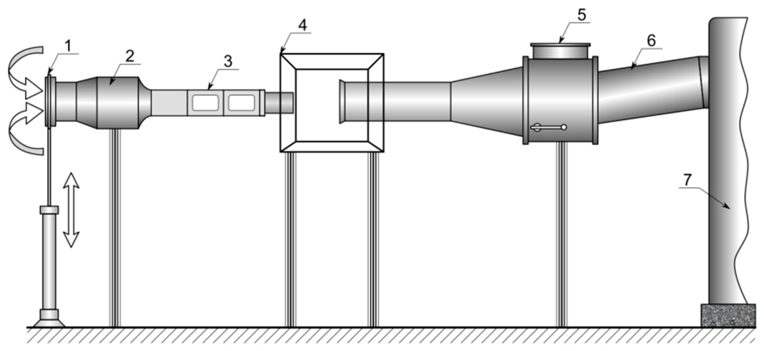
The experimental data were used for the analysis published by the authors earlier in [29] as well as the results of new experiments obtained with the usage of a similar experimental setup. The working part of the experimental setup (Figure 1) is a channel of constant cross-section (transverse dimensions 75 × 75 mm) with a supersonic air flow.

Figure 1.
General view of the experimental setup: 1—pneumatic valve; 2—receiver; 3—working chamber with the supersonic insert and water supply to the stream; 4—vacuum chamber, 5—vacuum seal, 6–gas flow path, 7—gas tanks.
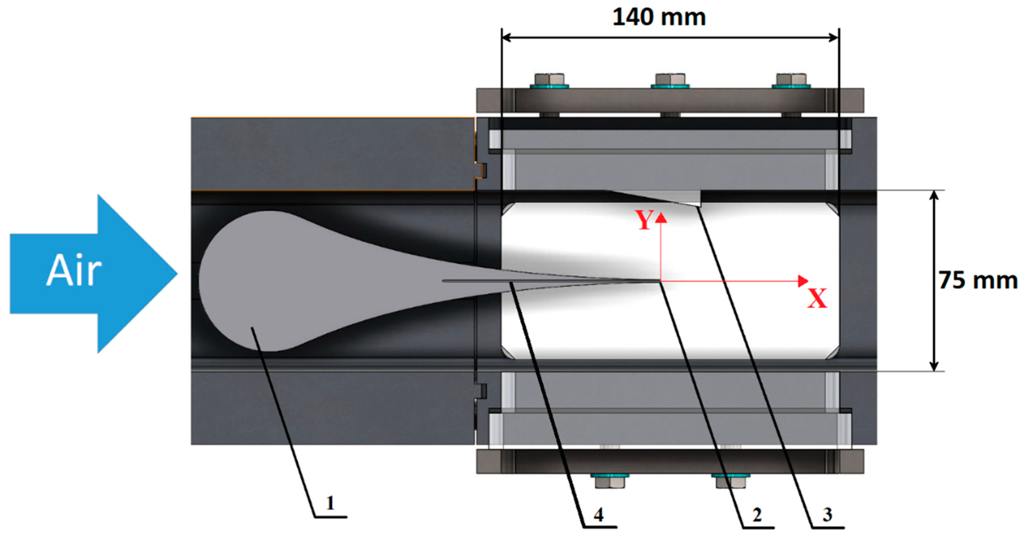
To obtain a supersonic flow at the inlet to the test section of the experimental setup, three different central aerodynamic nozzles were installed (the setup scheme is shown in Figure 2). These nozzles were designed to generate a flow with Mach numbers in the range from 2 to 3 with a step of 0.5. Let us take the following designations in the text: nozzle 1 corresponds to the calculated Mach number M = 2, nozzle 2 corresponds to the calculated Mach number M = 2.5, nozzle 3 corresponds to the calculated Mach number M = 3. The configuration of the nozzles is selected on the profiling basis by the method of characteristics with respect to the growth of the boundary layer. The criterion for choosing the nozzle profile was the uniformity of the flow in the outlet section. To implement the flow with oblique shock waves the special wedge with an angle of 10° relative to the axis of the experimental setup working part was installed on the upper wall of the channel behind the nozzle.

Figure 2.
The layout of the wedge in the experimental setup: 1—central aerodynamic nozzle; 2—nozzle for water supply; 3—wedge; 4—water supply channel.
In the end part of all aerodynamic nozzles, there was an orifice with a diameter of d = 0.7 mm, through which water was injected co-directionally with the air flow at supply pressures from pliquid = 0.6 MPa to pliquid = 1.6 MPa. The length of the orifice in all nozzles was ~100 mm.
Particle Image Velocimetry (PIV) measurements were carried out to confirm the distribution of the flow velocity in the duct during preliminary investigation without liquid injection [30]. To register tracers a video camera with a resolution of 1600 × 1200 pixels was installed in the mode of the double exposure with a delay of 3 … 8 μs. To illuminate the tracers we used a laser knife based on a double Nd:YAG laser with a 532 nm second harmonic generator and an energy in one pulse up to 125 mJ. The measurement frequency was up to 10 Hz.
Taking into account the preliminary approbation carried out for high velocity flows the shadow method was used in the experiments at the diagnostic method of liquid droplet parameters [31]. The mentioned method makes it possible to determine the droplet velocity vector and droplet diameter. The minimum recognizable droplet size that can be recognized by the equipment was 5 µm. The measurements were carried out in two areas (1 initial, 2 final). The dimensions of each measurement area were up to 2 mm × 2 mm. The coordinates of the centers of the measuring regions for different modes are presented in Table 1. Some differences in the coordinates of the measuring regions are associated with the peculiarities of the flow (shock wave and droplet trajectories). The position of the water injector nozzle corresponds to the coordinate (0,0).

Table 1.
Coordinates of measurement areas.
Within the framework of the present work 6 experiments without water supply (M = 2, M = 2.5, M = 3; without wedge and with it) were carried out to confirm the correspondence of the gas-dynamic flow parameters to the calculated ones, as well as three starts for each nozzle with different water injection pressures. The launches were carried out both with the installed wedge and without it (18 modes). Each of the experiments was repeated several times to obtain reliable data and their averaging. The results of the experiments were the distributions of droplet diameters and their velocities in the regions under consideration. The data obtained are presented in Appendix A.
It can be noted the following features of the obtained experimental regularities. The distribution of droplet diameters in region 2 is characterized by a decrease (relative to region 1) in the number of large diameter droplets (20 … 40 µm) and an increase in the proportion of fine droplets (≤10 µm). This indicates the process of droplet fragmentation due to their gas-dynamic breakup. It should be noted that the presence of an oblique shock wave has an ambiguous effect on the dispersion of droplets in region 2. At Mach numbers up to 2.5 for almost all liquid pressures in front of the nozzle, the oblique shock wave leads to a decrease in the rate of gas-dynamic breakup. This is due to decrease in the gas velocity behind the oblique shock wave and decrease in the relative Weber number. At Mach number M = 2.5 and p = 1.6 MPa, the effect of the presence of shock wave is practically leveled. An increase in the gas velocity leads to some intensification of the droplet destruction process resulting in smaller droplets formation. The droplets have a lower velocity difference relative to the gas flow. In this case the presence of an oblique shock wave intensifies fragmentation due to an increase in the relative Weber number behind it. Such effect is most noticeable for a liquid pressure in front of the nozzle of 0.6 MPa. The droplet size for higher liquid pressure drops in the nozzle reduces even more, the Weber numbers become lower and the effect of the oblique shock wave presence is leveled.
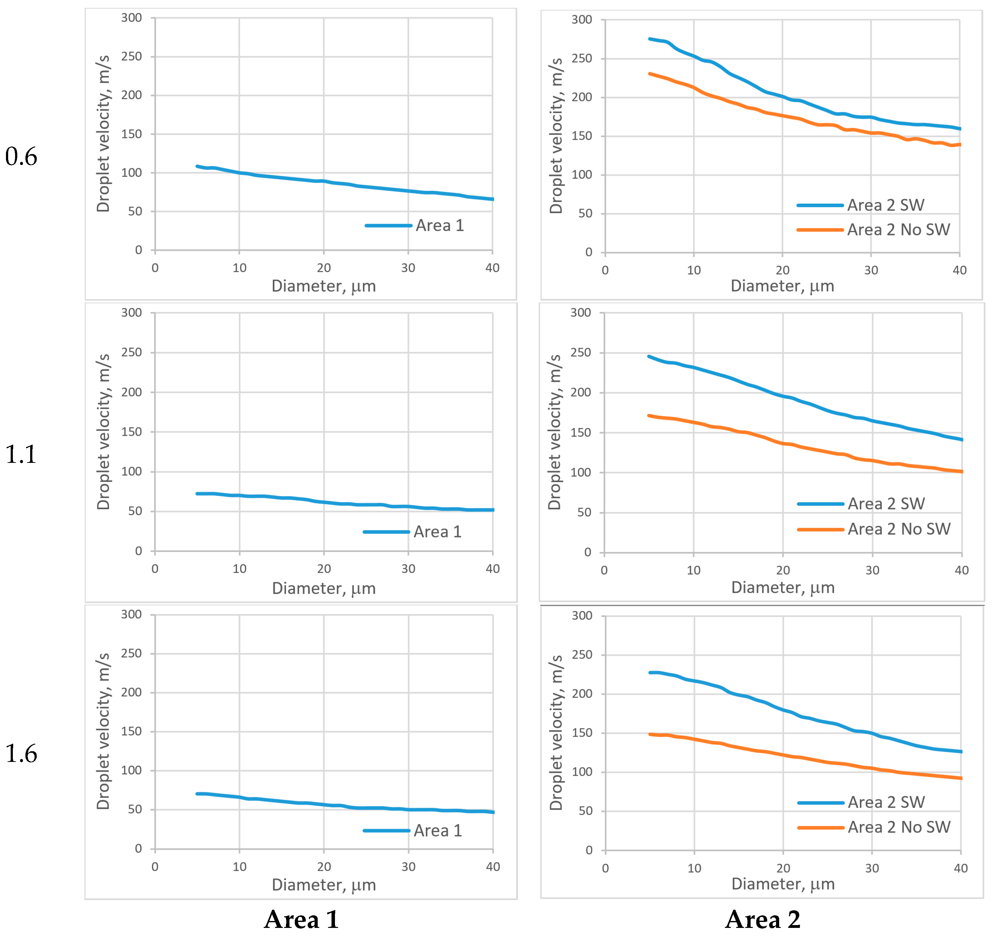
The droplet velocities also have some peculiarities depending on the flow regimes. The increase in the Mach number in particular leads to the decrease in the droplet velocity in region 1 from values (for droplets with a dimension of 5 μm) ~200 m/s at M = 2 to ~100 m/s at M = 3. This is due to the decrease in the static pressure and the dynamic pressure of the flow with an increase in the Mach number. An increase of fluid pressure in front of the nozzle leads to an increase in water mass flow rate. An increase in the mass flow rate of water injected at a relatively low velocity (below the gas velocity) leads to a local decrease in the two-phase flow velocity. This is due to the gas flow momentum decreasing. A similar situation is observed for the droplet velocities in region 2. It should be noted that the presence of an oblique shock wave at M = 2 leads to the increase in the droplet velocity in region 2, whereas at other Mach numbers it leads to its decrease. This can be explained by the fact that at M = 2 the velocity decrease in the shock wave is small and an increase in the static pressure behind it leads to an increase in the dynamic pressure. At higher Mach numbers the shock wave intensity increases, the velocity behind it decreases more significantly and the total pressure losses increases. It leads to the decrease in the aerodynamic force acting on the droplets.
The obtained experimental data were used to determine the regularities of the gas-dynamic breakup of droplets.
2.2. Numerical Simulation of the Gas Phase
To determine the parameters of the gas phase along the droplet trajectory a numerical simulation of the flow in a model channel was carried out for the three considered nozzles.
The calculation was carried out in the three-dimensional setting using a program based on solving the Navier-Stokes equations by the finite volume method. The research was carried out within the framework of the RANS approach using the γ-Reө SST turbulence model [32]. Gas properties correspond to air and depend on temperature and pressure. It should be noted that the calculation was performed without the presence of liquid droplets, which can change the flow structure and the distribution of parameters.
The unstructured mesh with a prismatic layer consisting of five cells was used. Along the oblique shock wave, as well as along the trajectory of the droplets, the mesh was condensed to the characteristic cubic cell size of 1 mm. The fluxes were calculated using the implicit AUSM scheme [33] of the second order of accuracy in space. The boundary conditions at the inlet are the total pressure of 0.1 MPa and the stagnation temperature of 300 K, at the outlet—the static pressure of 0.002 MPa. It was assumed that the walls of the channel and nozzle are adiabatic.
Figure 3 shows the distribution of Mach numbers for three nozzles without and with wedge-shaped insert. Figure 3a shows measuring regions 1 and 2, for which droplet distributions were recorded in the experiment.
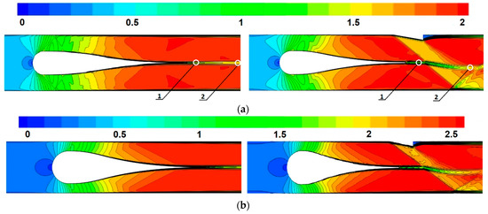
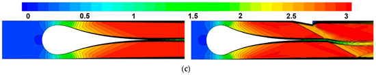
Figure 3.
Mach number fields without (left) and with (right) oblique shock wave. (a) nozzle 1, (b) nozzle 2, (c) nozzle 3.
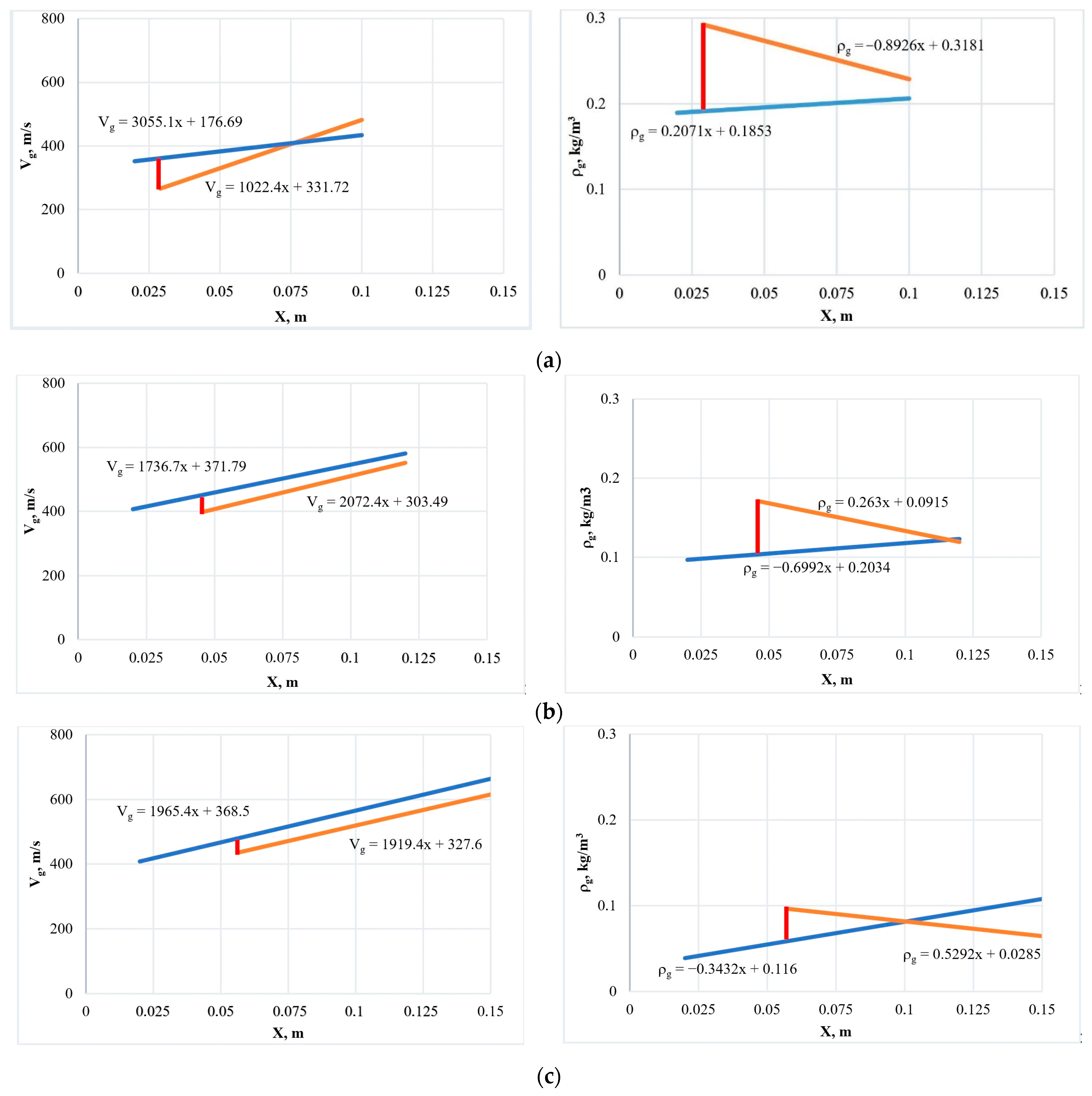
Based on the results of calculations several dependences were obtained. These regularities describe the change of the velocity Vg and density ρg of the gas along the trajectories of the droplets (Figure 4). The velocity and density functions are approximated by linear regularities, equations of which are shown in the graphs. The function for the entire breakup area for calculations without wedge corresponds to the blue graph. The piecewise-linear regularities corresponding to the blue curve before the shock wave and the orange one after are used for the calculation with a wedge. The vertical red line shows the shock wave location.
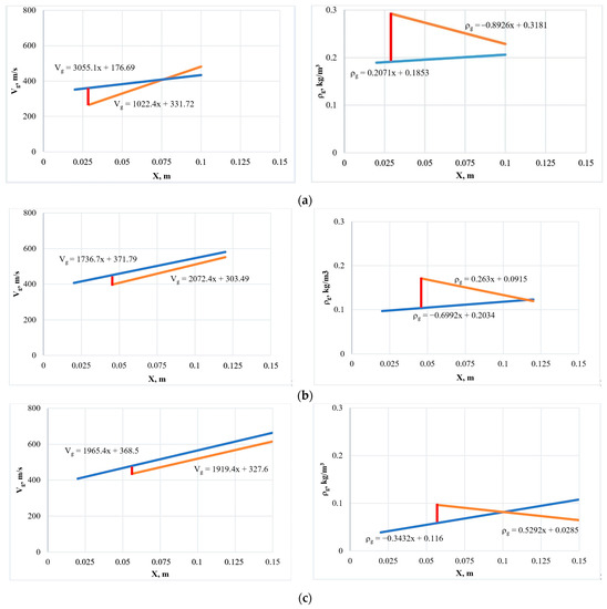
Figure 4.
Distribution of velocity (left) and density (right) of the gas phase along the trajectory of the droplets: blue lines-parameters without shock wave; red lines-parameters behind the oblique shock wave. (a) nozzle 1, (b) nozzle 2, (c) nozzle 3.
It should be noted that gradual increase in the gas velocity along the droplet trajectories is a consequence of the presence of a boundary layer formed at the central aerodynamic nozzle. As it moves the trace from the boundary layer is blurred and the gas is accelerated to the value close to the average flow velocity. This is also the reason of altering flux density.
An oblique shock wave results in increasing of static pressure and density as the gas velocity decreases. That is why a linear distribution function of parameters can be used in regimes without shock wave while shock wave leads to the necessity of using a piecewise-specified function with a discontinuity at the point of intersection of droplet trajectories with shock wave. The change of velocity at the point where the droplet trajectory is intersected by an oblique shock wave can be about 100 m/s, and the gas density can be about 0.1 kg/m3. The coordinate of the intersection of the droplet and shock wave trajectories for different Mach numbers is in the range from 0.01 to 0.04 m.
2.3. Description of Data Processing Methods
The proposed method for processing the experiment is aimed to establish physical and mathematical model for predicting the rate of gas-dynamic breakup of droplets in a supersonic flow.
Within the framework of the proposed method, the analysis of the change in the countable distribution of droplet diameters between region 1 and region 2. The change in the mass of the liquid due to evaporation was not taken into account since the temperature of the gas flow in the experiment [29] is lower than the boiling point of water. It should be noted that water crystallization was also not observed in the considered experiments.
The input parameters for the used mathematical model were the distributions of the droplet number and velocity modulus in measuring regions 1 and 2, in which the parameters were recorded. The minimum-recorded droplet diameter was 5 μm in the carried-out experiment, therefore, in the mathematical model the calculation was performed for droplet diameters from 5 to 85 μm. The velocity and temperature of submicron droplets practically coincided with similar parameters of the gas phase and their total mass did not exceed 10% of the mass of the supplied liquid; therefore, the absence of droplets with submicron diameters in calculations can be considered acceptable. During the analysis, the droplets were divided into groups according to fractions. The range of droplet diameters for each fraction was ∆ = 3 μm.
The used algorithm allows predicting the distributions of drop diameter and velocity in region 2 according to the distribution of parameters in region 1. In the case of an appropriate choice of mathematical regularities of gas-dynamic fragmentation of drops, the calculated and experimental distributions of parameters by drops in region 2 will have minimal discrepancies.
According to the results of published works [1,22,23] it was found out that the important factors affecting the destruction of droplets are: the initial diameter of the droplets, the relative velocity of the droplets, the presence of shock wave in the structure of the gas flow, as well as the physical and thermodynamic parameters of the liquid and gas.
To predict the distribution parameters in region 2, we used an explicit iterative method for calculating the droplet parameters for each elementary segment of the path. The calculation method is similar to the method described in [18].
To implement the numerical algorithm the path length L between the two measuring regions was divided into N elementary segments. The values of the gas parameters (velocity, density, pressure, temperature) for the elementary segment j were considered constant and corresponded to the calculated values in the center of the segment obtained as a result of the numerical simulation of the flow described above. It should be emphasized that at the point of intersection of droplet trajectories with the oblique shock wave the functions had a discontinuity of the first kind.
It is taken into account in the work that the coefficients of dynamic viscosity µg and thermal conductivity λg for gas depend on temperature. The coefficient of surface tension of water σl is constant σl = 7.2∙10−2 N/m. This is a consequence of an insignificant change of the droplet temperature in the flow (the droplet temperature in experiments changes by no more than 20 K). The mathematical model makes it possible to introduce the regularities of σl of the temperature of liquid droplets if necessary. In this case, the droplet temperature can be determined according to [18].
The calculation of the relative velocity of the drop with a diameter d Vrel = Vl − Vg (here Vg is the gas velocity and Vl is the velocity of the liquid in the coordinate system of the experimental setup) was carried out by integrating the differential equation:
where —drop cross-sectional area; Cx droplet drag coefficient; t—time. Hereinafter, the index “g”—corresponds to the parameters of the gas, and “l” to the parameters of the liquid.
The Reynolds, Weber, and Laplace numbers on an elementary path segment j for a drop were calculated by the formulas:
D32—the average volumetric surface (Sauter’s) diameter of the droplets for the fraction under consideration.
To calculate the drag coefficient Cx, the modified formula from [18] was proposed:
The first two factors in Equation (9) determine the aerodynamic drag coefficient of spherical droplet under various flow conditions, and the third factor is responsible for the effect of the droplet shape deviation from spherical.
According to the modes of the experiments carried out it can be assumed that for the cases under consideration fragmentation occurs according to three mechanisms: bag, shear stripping and vibration.
The bag type of breakup is characterized by the detachment of fragments from the edges of the droplet and is realized at Weber numbers We < 1.7∙104∙Lp. In this case, the average diameter of the detached fragments, according to [18], is represented by
In other cases, a shear stripping breakup is assumed due to the development of the Kelvin-Helmholtz instability. From the crests of disturbances (waves) appearing on the surface of the liquid, the separation of fragments begins, the diameters of which d1 are estimated by a value proportional to the average wavelength λ of these disturbances:
For Weber numbers 8 ≤ We ≤ 12, the transition to a relatively low-speed vibration type of gas-dynamic breakup is accepted [16]. At We ≤ 8, it was assumed that droplet fragmentation ceased. Thus, the critical Weber number for all calculations in accordance with the above Wecrit = 8. The obtained value of the critical Weber number agrees in order with the work [34] (Wecrit = 5.9), and also agrees with the range Wecrit = 4.20 also described in [34].
The breakup mechanisms occurring at high Weber numbers (We > 350) [35] (catastrophic breakup) were not realized within the framework of the experiment.
It is assumed that the fraction of droplets with a Weber number less than Wecrit did not change. For droplets with We ≥ Wecrit the change in their proportion was calculated using the formula proposed by the authors:
Here Pi is the relative number of particles of the considered fraction i; and - empirical coefficients. In the proposed model a set of parameters determines the number of particles separated from the droplet per unit time.
In this case, it is assumed that the fragments detached from the droplets of the considered fraction move as independent droplets into a fraction with a diameter d1.
The influence of the Re number for the breakup process is important since this parameter characterizes the effect of turbulent flow features. In addition, as shown in [36,37] the Re number affects the droplet shape—the surface area of the liquid film correlates with the Re number. A similar effect was noted in a numerical study [5]. The work [8] describes the classification of droplet destruction modes depending on the Re number. In particular, a change in Re leads to a shift in the boundary denoting the bag and shear stripping types of drop destruction.
The droplet velocity was calculated based on the obtained value of Cx, the direction of the velocity vector, as well as the density and velocity of the gas phase in the corresponding longitudinal coordinate. It is assumed that droplet fragments obtained as a result of gas-dynamic fragmentation at the moment of their formation have a velocity equal to the velocity of the initial droplet.
The distribution of diameters and droplet velocities in region 2 was determined based on the simulation results. Depending on the coefficients and , an array of relative counting distributions of droplet diameter and velocity was formed. An automated search of solution, which is in the most extent similar to the experimental data, was realized in this array. The criterion of maximum coincidence is the minimum value of the standard deviation Er between the calculated and experimental distributions in the relative number of particles (P) for different fractions in the measurement region 2:
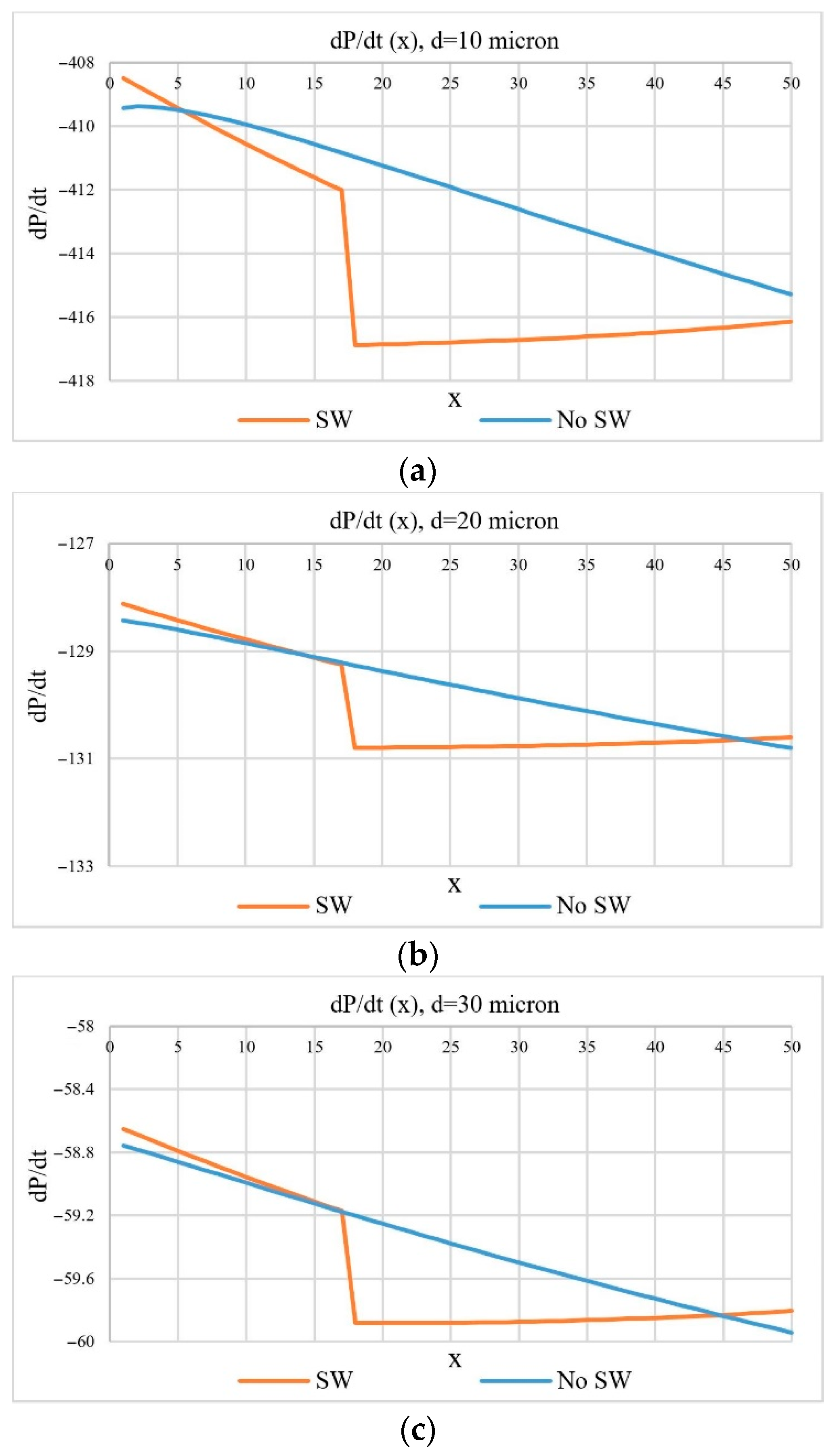
where M is the number of fractions, P(,)i—simulated relative number of droplets of the fraction i, (Pexp)i—the experimentally recorded relative number of drops of the fraction i, Norm is the normalizing coefficient. The normalizing factor is introduced due to the fact that droplets with a diameter less than dmin = 5 μm were not taken into account. Therefore, in order to properly estimate the relative number of droplets with a diameter of more than 5 μm it is necessary to normalize it to the Norm factor (usually ≤0.8) which depends on the proportion of unaccounted for droplets. The graphs of the change in the relative probability of finding droplets of three fractions from the longitudinal coordinate are shown in Figure 5.
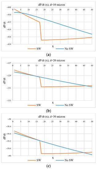
Figure 5.
The droplet breakup rate by the longitudinal coordinate. Blue line shows parameters without shock wave; red line—parameters with the shock wave. (a) d = 10 micron, (b) d = 20 micron, (c) d = 30 micron.
3. Analysis of Results
Analysis of the influence of the coefficients and on the characteristics of gas-dynamic breakup and comparison of calculations with experimental data allowed us to select the quantitative values of these coefficients, which for each experiment are shown in Table 2, Table 3 and Table 4. The tables also show the error value Er, which does not exceed 3.6%.
Table 2.
Coefficients of the mathematical model at M = 2.0.
Table 3.
Coefficients of the mathematical model at M = 2.5.
Table 4.
Coefficients of the mathematical model at M = 3.0.
It is seen that the coefficient tends to decrease with increasing pressure of liquid injection. It is also worth noting that the smaller the flow Mach numbers the values of are larger.
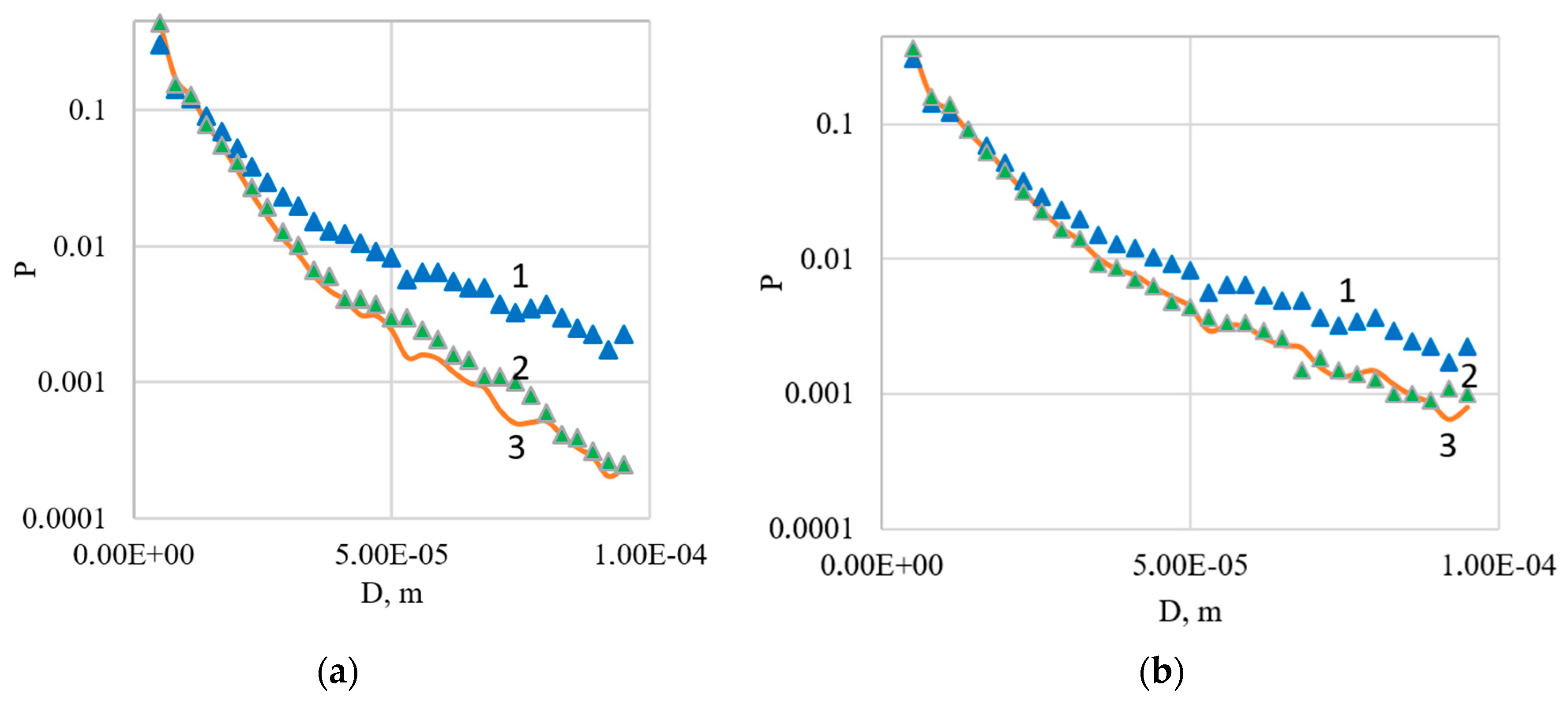
For example, in Figure 6 shows the experimental and simulated droplet distribution for one of the modes (M = 2.5; pl = 1.1 MPa) in the absence and presence of an oblique shock wave. For the same regime in Figure 6 shows a comparison of the droplet velocity distributions. It can be seen from the figures that the calculated and experimental distributions of diameters and velocities coincide practically qualitatively and quantitatively. The coincidence is also preserved in the presence of an oblique shock wave, taken into account in the calculation.
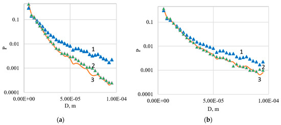
Figure 6.
The example of fractional distribution without shock wave (a) and with shock wave (b): 1—experimental distribution in area 1; 2—experimental distribution in area 2; 3—calculated distribution in area 2.
In Figure 6 and Figure 7 points mark experimental distributions, lines-calculated ones. The difference between calculations and experiments for this case does not exceed 0.8%.
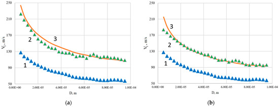
Figure 7.
The example of the distribution of droplet velocities without shock wave (a) and with shock wave (b): 1—experimental distribution in area 1; 2—experimental distribution in area 2; 3—calculated distribution in area 2.
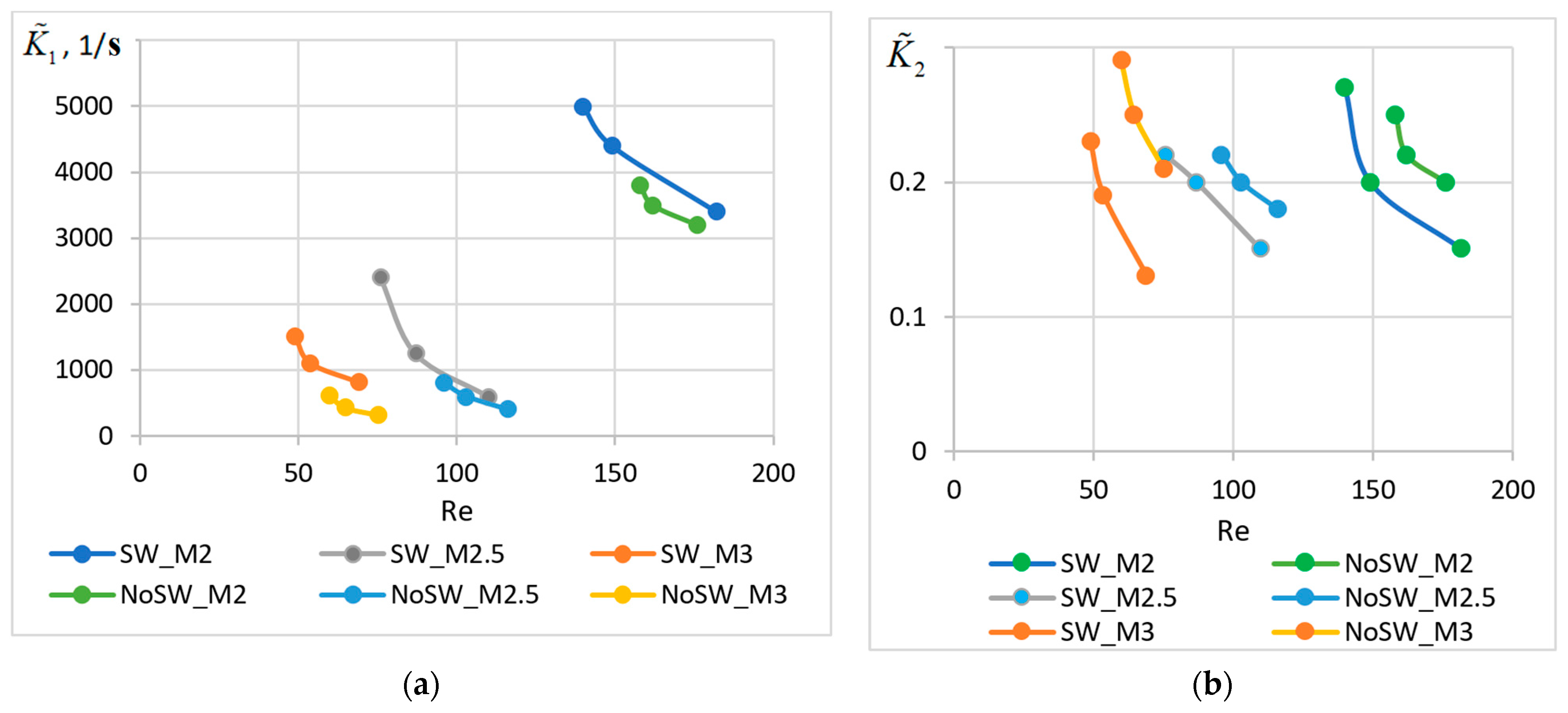
The dependences of the coefficients and on the trajectory-averaged Re number for drops were obtained. While maintaining the Mach number, an increase in the Reynolds number is achieved by increasing the injection pressure of the liquid. The Re number was averaged taking into account the mass fraction of each fraction.
Figure 8 shows that the obtained distributions of the coefficient values have a dependence close to exponential. This tendency manifested itself regardless of the presence or absence of shock wave. With an increase in the Mach number of the flow, the coefficient decreased.
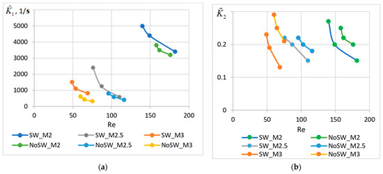
Figure 8.
Dependence of coefficients (a) and (b) on Re.
Analysis of the data obtained showed that the coefficient can be approximated by the following function:
where α = 4 × 10³, β = −0.136 × ln(M) + 0.0837, γ = 311.79 × ln(M) − 367.78.
There is a tendency for the coefficient to decrease with an increase in the water injection pressure. Taking into account that the influence of the considered factors on the coefficient is not significant, it can be taken equal to ~0.2 for the practical tasks. The proposed dependences for the coefficients and work both for cases with the presence of a shock wave and without the shock wave in a gas stream.
4. Conclusions
As a result of physical and mathematical modeling of the interaction of water droplets with a high-speed gas flow, the following was established.
- 1.
- The piecewise-specified function of the gas velocity and density distribution along the trajectory of liquid droplets with a discontinuity at the intersection of the droplet trajectories with an oblique shock wave can be used for one-dimensional calculations. The velocity and gas density changes at the point where the trajectory of a drop with an oblique shock wave is intercepted can be about 100 m/s and 0.1 kg/m3, respectively. The coordinate of the intersection of the droplet trajectories and shock wave for the considered experimental setup is in the range from 0.01 to 0.04 m depending on the flow Mach number.
- 2.
- The presence of an oblique shock wave has an uncertain effect on the rate of liquid droplets gas-dynamic breakup. An oblique shock leads to a decrease of the gas velocity and corresponding decrease of the gas-dynamic breakup rate for almost all pressures of liquid supply in front of the nozzle at Mach numbers less than 2.5. The increase of flow velocity to M = 3 leads to the process of destruction of drops behind the shock wave intensification.
- 3.
- On the basis of a comprehensive analysis of the calculated and experimental data the mathematical model that describes the intensity of gas-dynamic destruction of droplets with a diameter of 5 to 85 microns in a flow with Mach numbers M = 2–3 is proposed. The mathematical model takes into account the influence of the Mach, Weber, Laplace and Reynolds numbers on the rate of gas-dynamic fragmentation of droplets in a high-speed flow. The proposed mathematical model gives a discrepancy with experiment of no more than 3.6%.
The obtained computational and experimental data and the proposed mathematical model make it possible to estimate the intensity of liquid droplets gas-dynamic breakup in high-speed flows.
Author Contributions
Conceptualization, K.A.; methodology, K.A.; validation, A.M. and A.S.; formal analysis, A.M., O.G. and K.A.; investigation, A.M. and O.G.; resources, A.S.; data curation, A.S.; writing—original draft preparation, A.M., O.G. and K.A.; writing—review and editing, A.M. and O.G. All authors have read and agreed to the published version of the manuscript.
Funding
This research was funded by the Russian Science Foundation Grant No. 19-49-02031 And the APC was funded by Grant No. 19-49-02031.
Institutional Review Board Statement
Not applicable.
Conflicts of Interest
The authors declare no conflict of interest.
Abbreviations
The following abbreviations are used in this manuscript:
| PIV | Particle Image Velocimetry |
| Nd:YAG | Neodymium-doped Yttrium Aluminum Garnet; Nd:Y3Al5O12 |
| RANS | Reynolds-Averaged Navier-Stokes |
| AUSM | Advection Upstream Splitting Method |
| SW | Shock Wave |
Appendix A
Here the experimental data are presented. The graphs show the range of droplet diameters from 5 to 40 μm. An experiment with a wedge corresponds to a curve labeled “SW” (Shock Wave), to an experiment without a wedge—“No SW”.
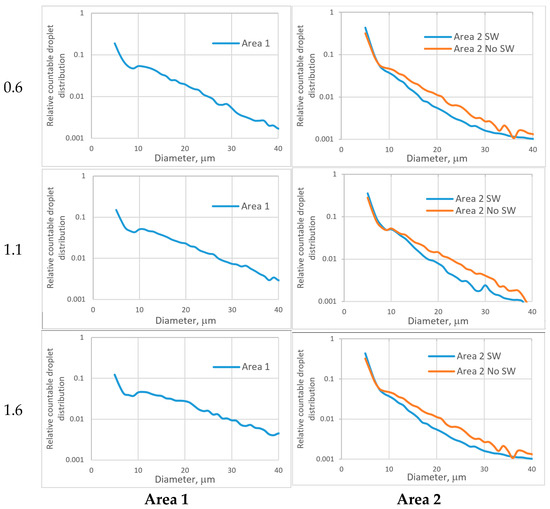
Figure A1.
Relative countable droplet distribution by diameters, gas flow Mach number M = 2. The left column shown water injection pressure pl, MPa.
Figure A1.
Relative countable droplet distribution by diameters, gas flow Mach number M = 2. The left column shown water injection pressure pl, MPa.
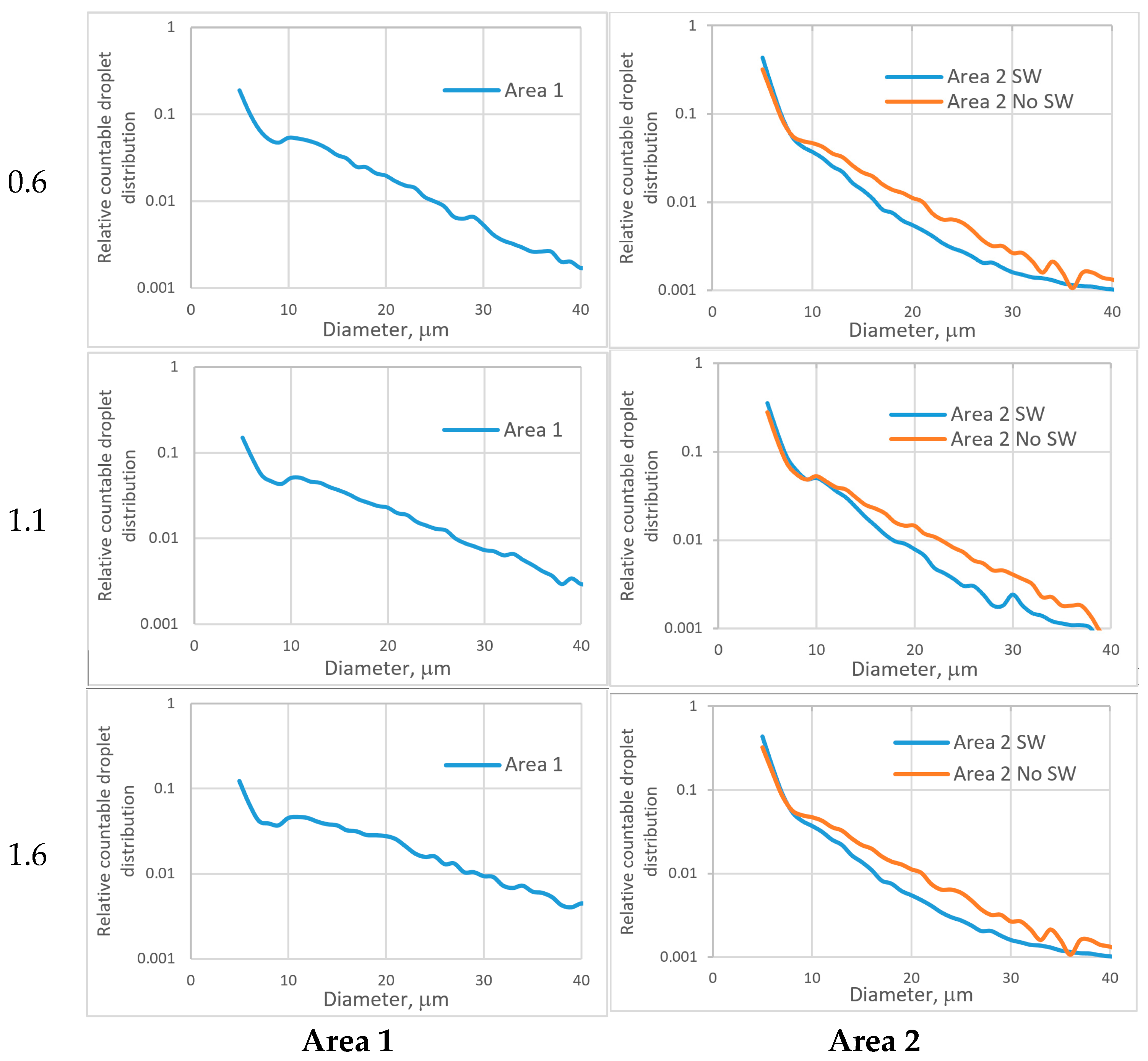
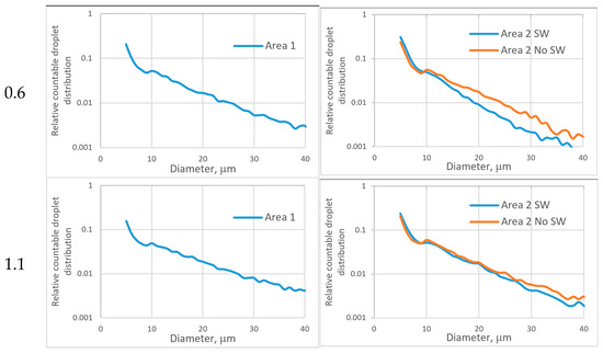
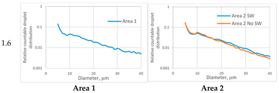
Figure A2.
Relative countable droplet distribution by diameters, gas flow Mach number M = 2.5. The left column shown water injection pressure pl, MPa.
Figure A2.
Relative countable droplet distribution by diameters, gas flow Mach number M = 2.5. The left column shown water injection pressure pl, MPa.
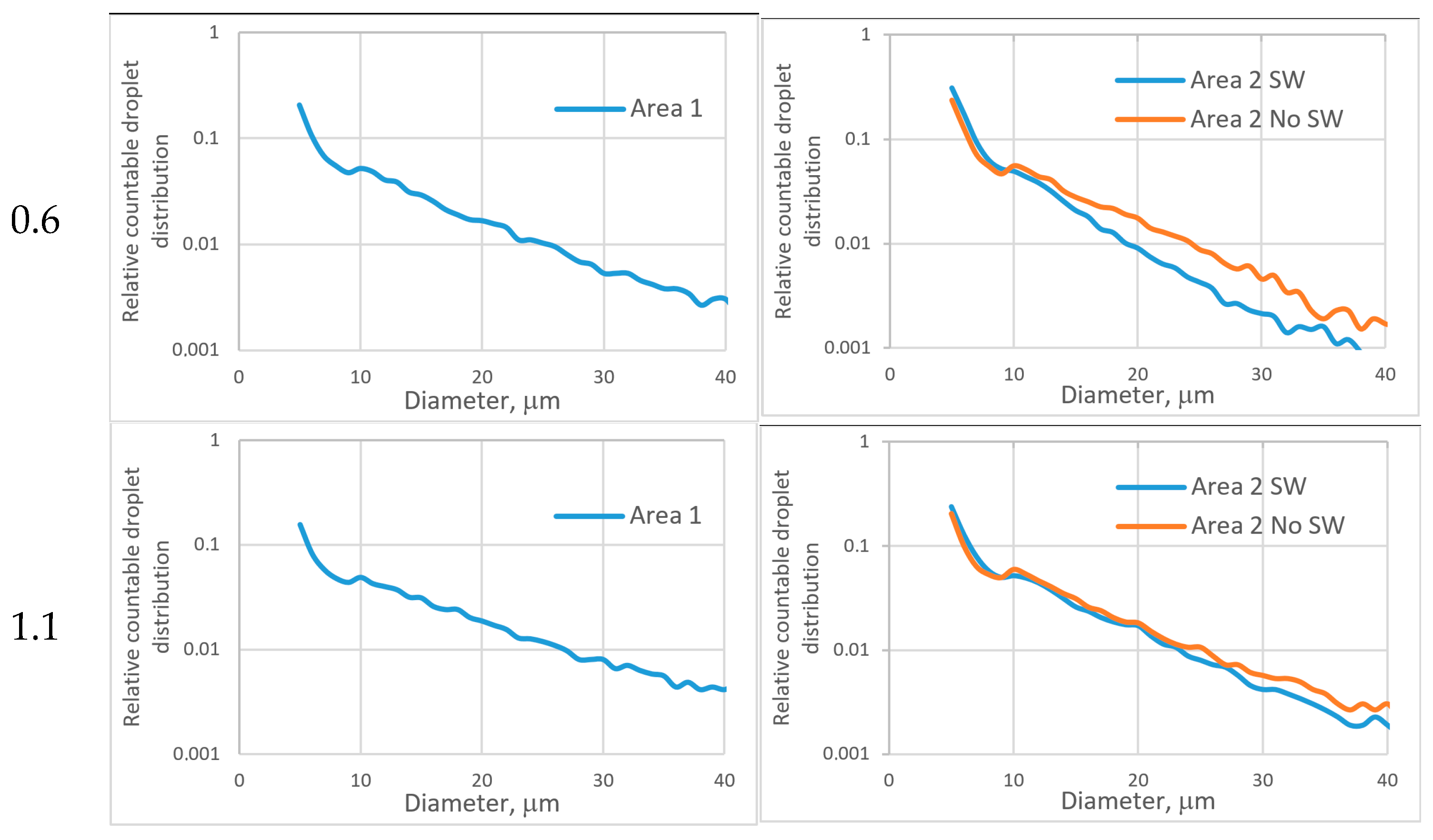

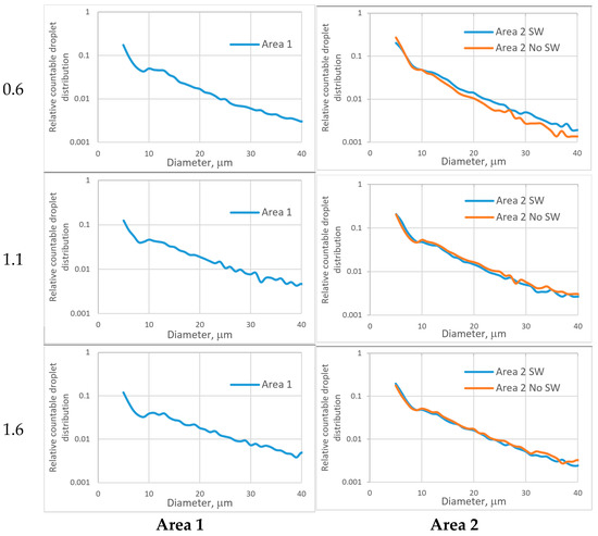
Figure A3.
Relative countable droplet distribution by diameters, gas flow Mach number M = 3. The left column shown water injection pressure pl, MPa.
Figure A3.
Relative countable droplet distribution by diameters, gas flow Mach number M = 3. The left column shown water injection pressure pl, MPa.
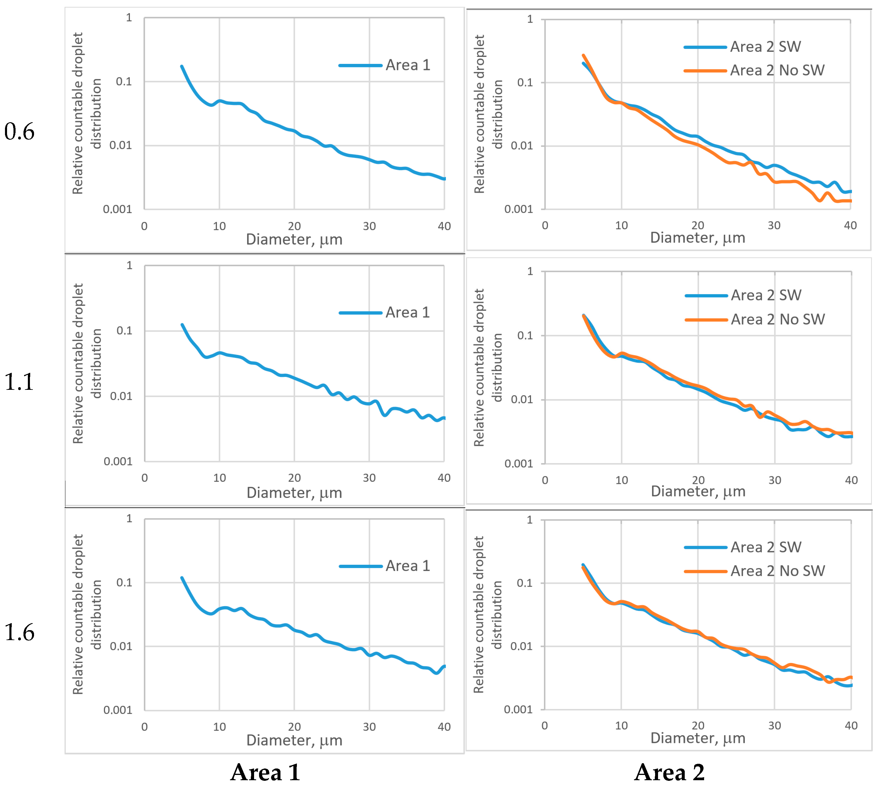
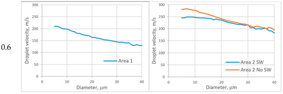
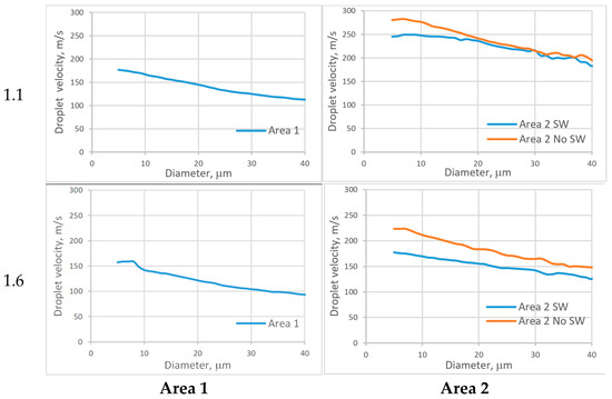
Figure A4.
Velocity distribution by droplet diameters, gas flow Mach number M = 2. The left column shown water injection pressure pl, MPa.
Figure A4.
Velocity distribution by droplet diameters, gas flow Mach number M = 2. The left column shown water injection pressure pl, MPa.
Figure A5.
Velocity distribution by droplet diameters, gas flow Mach number M = 2.5. The left column shown water injection pressure pl, MPa.
Figure A5.
Velocity distribution by droplet diameters, gas flow Mach number M = 2.5. The left column shown water injection pressure pl, MPa.
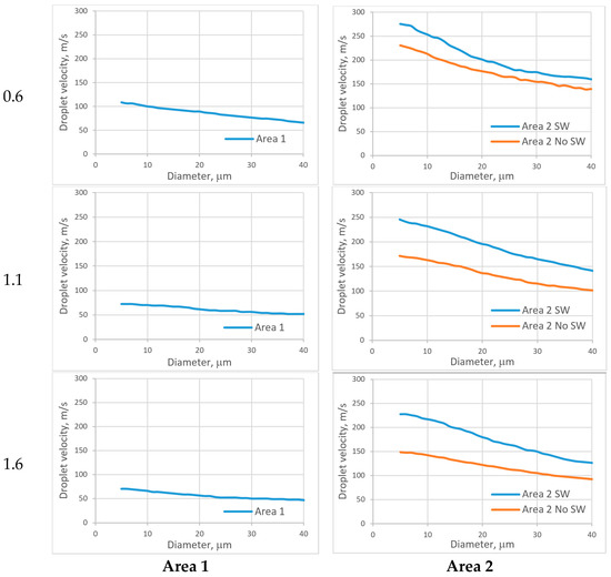
Figure A6.
Velocity distribution by droplet diameters, gas flow Mach number M = 3. The left column shown water injection pressure pl, MPa.
Figure A6.
Velocity distribution by droplet diameters, gas flow Mach number M = 3. The left column shown water injection pressure pl, MPa.
References
- Theofanous, T.G.; Li, G.J. On the Physics of Aerobreakup. Phys. Fluids 2008, 20, 052103. [Google Scholar] [CrossRef]
- Shao, C.; Luo, K.; Yang, Y.; Fan, J. Direct numerical simulation of droplet breakup in homogeneous isotropic turbulence: The effect of the Weber number. Int. J. Multiph. Flow 2018, 107, 263–274. [Google Scholar] [CrossRef]
- Shao, C.; Luo, K.; Fan, J. Detailed numerical simulation of unsteady drag coefficient of deformable droplet. Chem. Eng. J. 2017, 308, 619–631. [Google Scholar] [CrossRef]
- Wang, Z.; Hopfes, T.; Giglmaier, M.; Adams, N.A. Effect of Mach number on droplet aerobreakup in shear stripping regime. Exp. Fluids 2020, 61, 1–17. [Google Scholar] [CrossRef] [PubMed]
- Kékesi, T.; Amberg, G.; Wittberg, L.P. Drop deformation and breakup. Int. J. Multiph. Flow 2014, 66, 1–10. [Google Scholar] [CrossRef]
- Dorschner, B.; Biasiori-Poulanges, L.; Schmidmayer, K.; El-Rabii, H.; Colonius, T. On the formation and recurrent shedding of ligaments in droplet aerobrakeup. J. Fluid Mech. 2020, 904, A20. [Google Scholar] [CrossRef]
- Marcotte, F.; Zaleski, S. Density contrast matters for drop fragmentation thresholds at low Ohnesorge number. Phys. Rev. Fluids 2019, 4, 103604. [Google Scholar] [CrossRef] [Green Version]
- Giffen, E.; Muraszew, A. The Atomization of Liquid Fuels; Chapman & Hall: London, UK, 1953. [Google Scholar]
- Hinze, J.O. Fundamentals of the hydrodynamic mechanism of splitting in dispersion processes. AIChE J. 1955, 1, 289–295. [Google Scholar] [CrossRef]
- Gelfand, B.E.; Silnikov, M.V.; Takayama, K. Destruction of Liquid Droplets; Polytechnic University Press: Saint Petersburg, Russia, 2008. (In Russian) [Google Scholar]
- Girin, A.G. Hydrodynamic instability and droplet fragmentation models. Eng. Phys. J. 1985, 48, 771–776. (In Russian) [Google Scholar] [CrossRef]
- Gobyzov, O.A.; Ryabov, M.N.; Bilsky, A.V. Study of Deformation and Breakup of Submillimeter Droplets’ Spray in a Supersonic Nozzle Flow. Appl. Sci. 2020, 10, 6149. [Google Scholar] [CrossRef]
- Gelfand, B. Droplet breakup phenomena in flows with velocity lag. Prog. Energy Combust. Sci. 1996, 22, 201–265. [Google Scholar] [CrossRef]
- Guildenbecher, D.R.; López-Rivera, C.; Sojka, P.E. Secondary atomization. Exp. Fluids 2009, 46, 371–402. [Google Scholar] [CrossRef]
- Pilch, M.; Erdman, C.A. Use of breakup time data and velocity history data to predict the maximum size of stable fragments for acceleration-induced breakup of a liquid drop. Int. J. Multiph. Flow 1987, 13, 741–757. [Google Scholar] [CrossRef]
- Sichani, A.B.; Emami, M.D. A droplet deformation and breakup model based on virtual work principle. Phys. Fluids 2015, 27, 32103. [Google Scholar] [CrossRef]
- Liu, N.; Wang, Z.; Sun, M.; Wang, H.; Wang, B. Numerical simulation of liquid droplet breakup in supersonic flows. Acta Astronaut. 2018, 145, 116–130. [Google Scholar] [CrossRef]
- Arefyev, K.Y.; Voronetsky, A.V. Modelling of the process of fragmentation and vaporization of non-reacting liquid droplets in high-enthalpy gas flows. Thermophys. Aeromech. 2015, 22, 585–596. [Google Scholar] [CrossRef]
- Voronetsky, A.V.; Suchkov, S.A.; Filimonov, L.A. Peculiarities of high-temperature two-phase flow of combustion products in channels with an intentionally structured system of shock-waves. Thermophys. Aeromech. 2007, 14, 201–210. [Google Scholar] [CrossRef]
- Abramzo, В.; Sirignano, W.A. Droplet vaporization model for spray combustion calculations. Int. J. Heat Mass Trans. 1989, 32, 1605–1618. [Google Scholar] [CrossRef]
- Sula, C.; Grosshans, H.; Papalexandris, M.V. Assessment of Droplet Breakup Models for Spray Flow Simulations. Flow Turbul. Combust. 2020, 105, 889–914. [Google Scholar] [CrossRef]
- Kucharika, М.; Shashkov, M. Conservative multi-material remap for staggered multi-material Arbitrary Lagrangian—Eulerian methods. J. Comput. Phys. 2014, 258, 268–304. [Google Scholar] [CrossRef]
- Theofanous, T.G.; Chang, C.H. On the computation of multiphase interactions in transonic and supersonic flows. In Proceedings of the AIAA-2008 Conference, Reno, NV, USA, 7–10 January 2008; p. 1233. [Google Scholar]
- Arefiev, K.Y.; Voronetsky, A.V.; Suchkov, S.A.; Ilchenko, M.A. Computational and experimental study of two-phase mixture formation in a gas-dynamic ignition system. Thermophys. Aeromech. 2017, 24, 225–237. [Google Scholar] [CrossRef]
- Betelin, V.B.; Smirnov, N.N.; Nikitin, V.F.; Dushin, V.R.; Kushnirenko, A.G.; Nerchenko, V.A. Evaporation and ignition of droplets in combustion chambers modeling and simulation. Acta Astronaut. 2012, 70, 23–35. [Google Scholar] [CrossRef]
- Li, P.; Wang, Z.; Sun, M.; Wang, H. Numerical simulation of the gas-liquid interaction of a liquid jet in supersonic crossflow. Acta Astronaut. 2017, 134, 333–344. [Google Scholar] [CrossRef]
- Reinecke, W.G.; Waldman, G.D. Shock layer shattering of cloud drops in reentry flight. AIAA Pap. 1975, 152, 22. [Google Scholar]
- Arefyev, K.Y.; Prokhorov, A.N.; Saveliev, A.S. Study of the breakup of liquid droplets in the vortex wake behind pylon at high airspeeds. Thermophys. Aeromech. 2018, 25, 55–66. [Google Scholar] [CrossRef]
- Arefyev, K.Y.; Guskov, O.V.; Prokhorov, A.N.; Saveliev, A.S.; Son, E.E.; Gauthame, K.; Same, D.; Sonu, K.T.; Muruganandame, T.M. Experimental research of gasdynamic liquid drops breakup in the supersonic flow with the oblique shock wave. High Temp. 2020, 58, 884–892. [Google Scholar] [CrossRef]
- Raffel, M.; Willert, C.E.; Scarano, F.; Kähler, C.; Wereley, S.T.; Kompenhans, J. Particle Image Velocimetry: A Practical Guide; Springer International Publishing: Berlin/Heidelberg, Germany, 2018. [Google Scholar]
- Settles, G.S. Schliren and Shadowgraph Techniques, 1st ed.; Springer: Berlin/Heidelberg, Germany, 2001. [Google Scholar]
- Menter, F.R. Two-Equation Eddy-Viscosity Turbulence Models for Engineering Applications. AIAA J. 1994, 32, 1598–1605. [Google Scholar] [CrossRef] [Green Version]
- Liou, M.S.; Steffen, C.J. A New Flux Splitting Scheme; Academic Press Professional Inc.: Cambridge, MA, USA, 1993. [Google Scholar]
- Pavlenko, I.; Sklabinskyi, V.; Doligalski, M.; Ochowiak, M.; Mrugalski, M.; Liaposhchenko, O.; Skydanenko, M.; Ivanov, V.; Włodarczak, S.; Woziwodzki, S.; et al. The Mathematical Model for the Secondary Breakup of Dropping Liquid. Energies 2020, 13, 6078. [Google Scholar] [CrossRef]
- Huang, X.; Liu, J.; Liao, S.; Wu, J. Experimental investigation of the deformation and breakup of a droplet in high-speed flow. Sci. Sin. Phys. Mech. Astron. 2018, 48, 054701. [Google Scholar] [CrossRef]
- Han, J.; Tryggvason, G. Secondary breakup of axisymmetric liquid drops. I. Acceleration by a constant body force. Phys. Fluids 1999, 11, 3650–3667. [Google Scholar] [CrossRef]
- Han, J.; Tryggvason, G. Secondary breakup of axisymmetric liquid drops. II. Impulsive acceleration. Phys. Fluids 2001, 13, 1554–1565. [Google Scholar] [CrossRef]


Publisher’s Note: MDPI stays neutral with regard to jurisdictional claims in published maps and institutional affiliations. |
© 2021 by the authors. Licensee MDPI, Basel, Switzerland. This article is an open access article distributed under the terms and conditions of the Creative Commons Attribution (CC BY) license (https://creativecommons.org/licenses/by/4.0/).