Research on Alarm Reduction of Intrusion Detection System Based on Clustering and Whale Optimization Algorithm

Abstract

With the frequent occurrence of network security events, the intrusion detection system will generate alarm and log records when monitoring the network environment in which a large number of log and alarm records are redundant, which brings great burden to the server storage and security personnel. How to reduce the redundant alarm records in network intrusion detection has always been the focus of researchers. In this paper, we propose a method using the whale optimization algorithm to deal with massive redundant alarms. Based on the alarm hierarchical clustering, we integrate the whale optimization algorithm into the process of generating alarm hierarchical clustering and optimizing the cluster center and put forward two versions of local hierarchical clustering and global hierarchical clustering, respectively. To verify the feasibility of the algorithm, we conducted experiments on the UNSW-NB15 data set; compared with the previous alarm clustering algorithms, the alarm clustering algorithm based on the whale optimization algorithm can generate higher quality clustering in a shorter time. The results show that the proposed algorithm can effectively reduce redundant alarms and reduce the load of IDS and staff.

1. Introduction

With the continuous development of computer network technology, people are more and more dependent on the convenience brought by the internet, but at the same time, the characteristics of the network, such as openness and complexity, also lead to the complexity and diversity of network security threats. In order to avoid the damage caused by network threats, many network security technologies are widely used, such as firewall, intrusion detection system (IDS), vulnerability scanning program and so on [1]. This study mainly focuses on the IDS, especially on how to improve the efficiency and performance of the IDS when dealing with network security events.

IDSs can be divided into two categories: the signature-based IDS and anomaly-based IDS [2]. The signature-based IDS determines whether network traffic shows malicious or normal behavior by maintaining a knowledge base [3]. The anomaly-based IDS detects whether the network traffic deviates from the normal rule state to determine malicious traffic [4]. Whether the signature-based IDS or the anomaly-based IDS can identify different types of network attacks is an important factor to judge its effectiveness. Therefore, the establishment of an intrusion detection system needs a network data set as the support. In past studies, many open network data sets were used by scholars as benchmark data sets, such as KDDCup99 [5] and NSL-KDD [6], which were widely used in various studies in the field of network security. However, with the rapid development of network technology and the emergence of new cyber security threats, these data sets have become outdated. In recent years, many new network data sets have been published on the internet, such as DDoS 2016 [7], UNSW-NB15 [8] and CICIDS 2017 [9]. Scholars are gradually using these relatively new data sets in their studies. Moreover, network data sets are still attracting the attention of scholars, such as LITNET-2020 [10], a new data set proposed by Damasevicius et al. based on the real network environment in 2020. These data sets usually have a fairly high-dimensional number of features, and different features may have different types, such as numerical type and categorical type. Due to the size of the data set, it is inevitable that there will be missing values in the data set. In the past, researchers proposed a series of methods, such as clustering, to deal with this problem [11,12,13].

According to literature statistics [14,15], the IDS will generate a large number of alarms in a very short period of time, 85% of which are irrelevant alarms or false alarms. In the past studies, many scholars have used different technologies to deal with the problem of redundant alarms generated by the IDS [16]. These methods can be generally divided into clustering-based methods [17,18,19], attribute-similarity-based methods [1,20], expert-system-based methods [21,22], genetic-algorithm-based methods [23,24], data-mining-based methods [25,26], etc.

Swarm intelligence optimization algorithms in recent years, as a kind of heuristic algorithm, are receiving more and more attention from researchers [27]. This kind of optimization algorithm is a good way to deal with the NP problem. The whale optimization algorithm (WOA), as an emerging swarm intelligence optimization algorithm, was proposed by Mirjalili and Lewis in 2016 [28]. Mirjalili and Lewis took inspiration from the behavior of humpback whales as they hunted their prey and modeled the process in the abstract into concrete mathematical equations. WOA is applied in many academic fields and achieves good results [29]. The specific application and theoretical background of WOA are described in detail in Section 2 and Section 3.

The main contributions and findings of this paper are as follows:

• To deal with the alarm reduction problem, we propose a coding and decoding scheme that applies WOA to hierarchical clustering and propose a new fitness function. We apply crossover and mutation operators to WOA to enhance the search capability of the algorithm.
• To solve the problems of premature convergence of clustering and the tendency of clustering algorithm to fall into the local optimum, we propose a local version of WOA applied to hierarchical clustering, namely WOAHC-L. On the basis of WOAHC-L, we further propose a global version of WOAHC to resolve the problem of the high overlap degree of the cluster center, namely WOAHC-G.
• We conducted experiments on UNSW-NB15 data set to explore the performance of WOAHC in the search of cluster centers, time consuming, clustering results, accuracy and other indicators. Compared with the alarm hierarchical clustering algorithm in the past, the proposed framework can obtain higher quality alarm clustering within the allowed time range and solves the problem of alarm redundancy well.

The structure of this paper is as follows: The second part introduces the related work. The third part provides the theoretical background and introduces the framework of hierarchical clustering and the method of alarm distance calculation. In the fourth part, we propose our new methods for alarm hierarchy clustering, named WOAHC-L and WOAHC-G. The fifth part carries on the experiment and provides the experiment result and our discussion. The sixth part is the conclusion of this paper.

2. Literature Review

In the previous section, we gave an overview of several categories of methods for dealing with redundant alarms. In this section, we mainly discuss hot approaches for dealing with alarm problems in recent years and explore the application of heuristic algorithms (such as WOA) in dealing with alarm problems in the intrusion detection domain. Firstly, we introduce the research results of scholars on alarm problems of the past few years. Wang et al. [30] proposed a framework to improve the intelligent false alarm reduction for DIDS based on edge computing devices. They built a false alarm filter by using machine learning classifiers, which can select an appropriate algorithm to maintain the filtration accuracy. Toldinas et al. [31] proposed a new image recognition method using multi-level deep learning to solve the problem of intrusion detection system identification of network attacks. They converted network features into four-channel images that were used to train and test the pre-trained deep learning model ResNet50. Kinghorst et al. [32] introduced a pre-processing step in the process of alarm flood analysis to enhance the robustness of the alarm system in dealing with the random alarm or interference alarm mode through probability calculation of alarm correlation. Fahimipirehgalin et al. [33] proposed a data-driven method, using alarm log files to detect the causal sequence of alarms. In this method, an efficient alarm clustering method based on the time distance between alarms is proposed, which is helpful to preserve adjacent alarms in a cluster. To solve the problem of a large number of redundant alarms generated by IDS, Sun and Chen [1] proposed an alarm aggregation scheme based on the combination of conditional rough entropy and knowledge granularity. Based on this scheme, the weights of different attributes in the alarms were obtained, and the similarity values of the alarms were calculated within the sliding time window to aggregate the similar alarms to reduce redundant alarms.

In recent years, the development of swarm intelligence optimization algorithms has attracted the attention of researchers. Swarm intelligence (SI) optimization algorithms can be divided into two main categories: one is the particle swarm optimization algorithm (PSO), and the other is the ant colony optimization algorithm (ACO). The emergence of SI was first used to solve optimization problems and was subsequently applied by scholars in the field of network attack detection. Alharbi et al. [34] proposed a method combining the bat algorithm and neural network to detect botnet attacks. The bat algorithm is used to select feature subsets and adjust hyperparameters in a network attack, and is used to adjust the hyperparameters and weight optimization of a neural network. In article [35], Khurma et al. combined the salp swarm algorithm and ant lion optimization algorithm to propose a wrapper feature selection model to solve the problem of high dimension of features in IDS. Zhang et al. [36] proposed an improved particle swarm optimization algorithm to solve the problems of repeated alarms and high false positive rate in IDS. In the process of reconstructing the attack path between DDoS attack victims and attackers based on an internet protocol backtracking scheme, Lin et al. [37] proposed a multi-mode optimization scheme that applied the improved locust swarm optimization algorithm to the reconstructed attack path in order to solve the problem that the traditional route search algorithm was prone to fall into local optimum. This method shows the excellent search performance of the SI algorithm. In addition, there is also a lot of research of SI in the feature selection stage of the IDS and attack target detection [38,39,40].

PSO and ACO algorithms have achieved good results in many fields. On this basis, scholars have proposed more excellent swarm intelligence optimization algorithms inspired by nature, such as the WOA [28], bat algorithm [41], wolf optimization algorithm [42], pathfinder algorithm [43], etc. Mirjalili and Lewis studied the behavior of humpback whales in preying on prey, analyzed and modeled the behavior patterns of the bubble net attack and spiral approach, and put forward the WOA. It is proved that the WOA has strong competitiveness, compared with the existing meta-heuristic algorithms and traditional algorithms. After WOA was proposed, due to its excellent problem optimization ability, it was quickly applied in various fields of research. In a review article on the application of WOA [29], the author listed the research progress of WOA, including hybridization, improvement and variation, as well as application scenarios such as engineering problems, clustering problems, classification problems, image processing, network and task scheduling and other problems. It can be seen that WOA, as a new meta-heuristic swarm intelligent optimization algorithm, has proved its reliability and good performance in handling optimization problems. However, in the field of alarm clustering, previous scholars did not carry out further research on it. Based on the proven global and local search capabilities of WOA, this paper studies the application of WOA in alarm clustering, focusing on the optimization of alarm hierarchical clustering based on WOA.

3. Theoretical Background

In this section, we introduce the relevant theoretical background of the study. Firstly, we introduce the alarm reduction algorithm based on hierarchical clustering, including the concept of generalization level, the calculation method of distance and the basic process of the algorithm. Second, we introduce the main ideas and basic process of WOA.

Table 1. Table of notations used in this paper.

Symbol	Description
$N_i$	$i\mathrm{th}$ node of a hierarchical tree
$A_i$	$i\mathrm{th}$ alarm in an alarm set
$D_{Ai-Aj}$	The distance between $i\mathrm{th}$ alarm and $j\mathrm{th}$ alarm in an alarm set
$C_i$	$i\mathrm{th}$ alarm cluster center
$\overrightarrow{X}\left(t\right)$	In WOA, the current solution at iteration t
$\overrightarrow{X^{*}}\left(t\right)$	In WOA, the best solution at iteration t
${\overrightarrow{X}}_{rand}$	In WOA, a random solution in the current solution space
$\overrightarrow{D}$	In WOA, the distance between $i\mathrm{th}$ $\overrightarrow{X}$ and $j\mathrm{th}\overrightarrow{X}$
$SearchAgents$	In WOA, the number of search agents to search solution simultaneously
$MaxIter$	In WOA, a predetermined maximum number of iterations
$C,r,a,l$	Random numbers used in WOA to control logical judgment
$E_{T}k\left(t,x\right)$	Fitness value of alarm number for cluster center k
$E_s\left(k\right)$	Fitness value of alarm distance for cluster center k
$O\left(C_i,C_j\right)$	The degree of overlap between $i\mathrm{th}$ cluster center $C_i$ and $j\mathrm{th}$ cluster center $C_j$
$E{S}_O$	Fitness value of the coincidence degree of all cluster centers in the cluster
$TP$	Number of normal network traffic clustering to normal cluster
$TN$	Number of network attack clustering to attack cluster
$FP$	Number of network attack alarms incorrectly clustering to normal cluster
$FN$	Number of normal network traffic incorrectly clustering to attack cluster

shows the list of notations used in this paper.

3.1. Alarm Reduction Algorithm Based on Hierarchical Clustering

3.1.1. Generalization Hierarchies

We first introduce the concept of generalization hierarchy. As mentioned earlier, if newly generated alarms are arranged in a meaningful cluster according to predefined rules, operators can easily understand what is happening in the network. According to this idea, we define the concept of cluster, and classify the alarms into the cluster they belong to according to the rules. We use the basic idea of hierarchical clustering proposed by Julisch [44,45]. As shown in Figure 1 below, for all the attributes in the alarm, we can use the method of hierarchical division to layer the attributes. Figure 1a shows the attribute hierarchical tree composed of IP attributes, and each leaf node of the tree represents a unique specific IP address. We can generalize it once to obtain the specific protocol using this IP, such as firewall and WWW/FTP in Figure 1a. If we continue to generalize it, we can obtain more advanced generalizations, such as DMZ and EXTERN. When we find that the generalization has reached the highest level and can no longer be generalized, we define the root of the hierarchy tree. For example, the root of the hierarchy tree to which the IP attribute belongs is ANY IP. The generalized structure of other attributes is similar, as shown in Figure 1b–d. In the past, scholars have proposed many methods for the construction of a hierarchical tree, with which we can construct a hierarchical tree for various attributes of the alarm data.

After providing the construction process of a hierarchical tree, we provide the following definitions of nodes in the hierarchical tree.

Definition 1.

A basic alarm is the alarm triggered by IDS that correspond to leaf nodes in the hierarchy tree. An abstract alarm is derived from the basic alarm by generalization and corresponds to intermediate or root nodes in the hierarchy number. Naturally, a basic alarm is also a special abstract alarm.

Definition 2.

In a hierarchical tree, if there is a path from$N_1$node to$N_2$node, then$N_1$is a generalization of$N_2$, and$N_2$is a specification of$N_1$.

Definition 3.

For both abstract alarms$A_1$and$A_2$,$A_1$is a generalization of$A_2$if each attribute in$A_1$is a generalization of the corresponding attribute in$A_2$, and at the same time,$A_2$is a specification of$A_1$.

Definition 4.

For an alarm set, the minimum cover refers to the common generalization of all alarms in the set, and the generalization is a minimum specification.

Based on the four definitions above, considering the four hierarchical trees shown in Figure 1, there is an alarm set that contains three alarms: $A_1$ (ip1,80,h1,11), $A_2$ (DMZ,80,h0,MIDDLE), and $A_3$ (DMZ, PRIVATE, WEEKEND, MIDDLE). $A_1$ is a basic alarm because all the attributes of the alarm are at leaf nodes in the hierarchical tree. $A_2$ and $A_3$ are abstract alarms because there is at least one attribute in the alarm that is the middle nodes in the hierarchy tree. $A_3$ is a generalization of $A_1$ and $A_2$ because every attribute of $A_3$ is a generalization of $A_1$ and $A_2,$ and obviously $A_3$ is a common generalization of $A_1$, $A_2$, and $A_3$.

3.1.2. Distance Definition

After obtaining the generalized alarm set, in order to cluster the alarms in the original alarm set, we need to define the distance calculation rule in the clustering problem, that is, defining the distance between two alarms to judge whether they belong to the same cluster. In fact, it is easy to calculate the distance between attributes of a numeric type, but there is a problem if the alarm property is a category, time, or string property using the same distance calculation method. We give the following definition to calculate the distance between two alarms in a hierarchical tree.

Definition 5.

The distance between any two nodes in the same hierarchical tree depends on the number of edges between them. If two nodes have directly linked edges, the distance between them is 1.

Definition 6.

If there is a generalization–specification relationship between two alarms, the distance between the two alarms is defined as the average distance between their attributes.

Definition 7.

The distance of an alarm set is defined as the average distance between the minimum coverage in the set and each alarm.

Consider the alarm sets $A_1$ (ip1,80,h1,11), $A_2$ (DMZ,80,h0,MIDDLE), and $A_3$ (DMZ, PRIVATE, WEEKEND, MIDDLE) mentioned above, where the minimum coverage in the alarm set is $A_3.$ The distance between $A_1$ and $A_2$ is (2 + 0 + 2 + 1)/4 = 1.25. The distance between the minimum coverage and alarm sets is (1.5 + 0.75 + 0)/3 = 0.75.

3.1.3. Definition of the Clustering Problem

The clustering method is now described as the following: among all triggered alarms, a group of generalized alarms is found; the number of alarms within each generalized alarm exceeds or is equal to a given threshold; and the distance between the alarms is as small as possible. This method is proved to be an NP complete problem, that is, the exact solution cannot be obtained in feasible time. Julisch presented an approximate algorithm [44] as shown in Algorithm 1.

Algorithm 1 Julisch’s alarm hierarchical clustering algorithm

Input: a set of events; a threshold T; a set of trees of all the attributes considerer; Output: an alarm/ /an abstract event 1: select an arbitrary alarm A, each member of which is a leaf in a tree 2: while the number of events A covers is less than T do 3:   select an arbitrary member of A, and replace the member with its direct parent 4: end while

3.2. Whale Optimization Algorithm

Mirjalili and Lewis proposed the whale optimization algorithm based on abstract modeling of the hunting strategies of humpback whales; it mimics the bubble-net feeding in the foraging behavior of humpback whales [28]. Humpback whales hunt close to the surface while trapping the prey in a net of bubbles. They create this net when swimming on a ‘6′-shaped path. The algorithm mimics two phases: the first phase (exploitation phase) is to encircle the prey and attack with spiral bubble nets, and the second phase (exploration phase) is searching randomly for prey. Figure 2 shows a series of behaviors of humpback whales as they hunt prey. Figure 2a shows the movement of the whale toward the prey, during which the whale can choose to move toward the lead whale or in a random direction. Figure 2b illustrates the shrinking encircling mechanism used by whales to capture prey. Besides the shrinking encircling mechanism, the whale also moves further toward the prey in a spiral shape, during which the whale emits a bubble attack to surround the prey, as shown in Figure 2c. The details of each phase are presented in the following subsections.

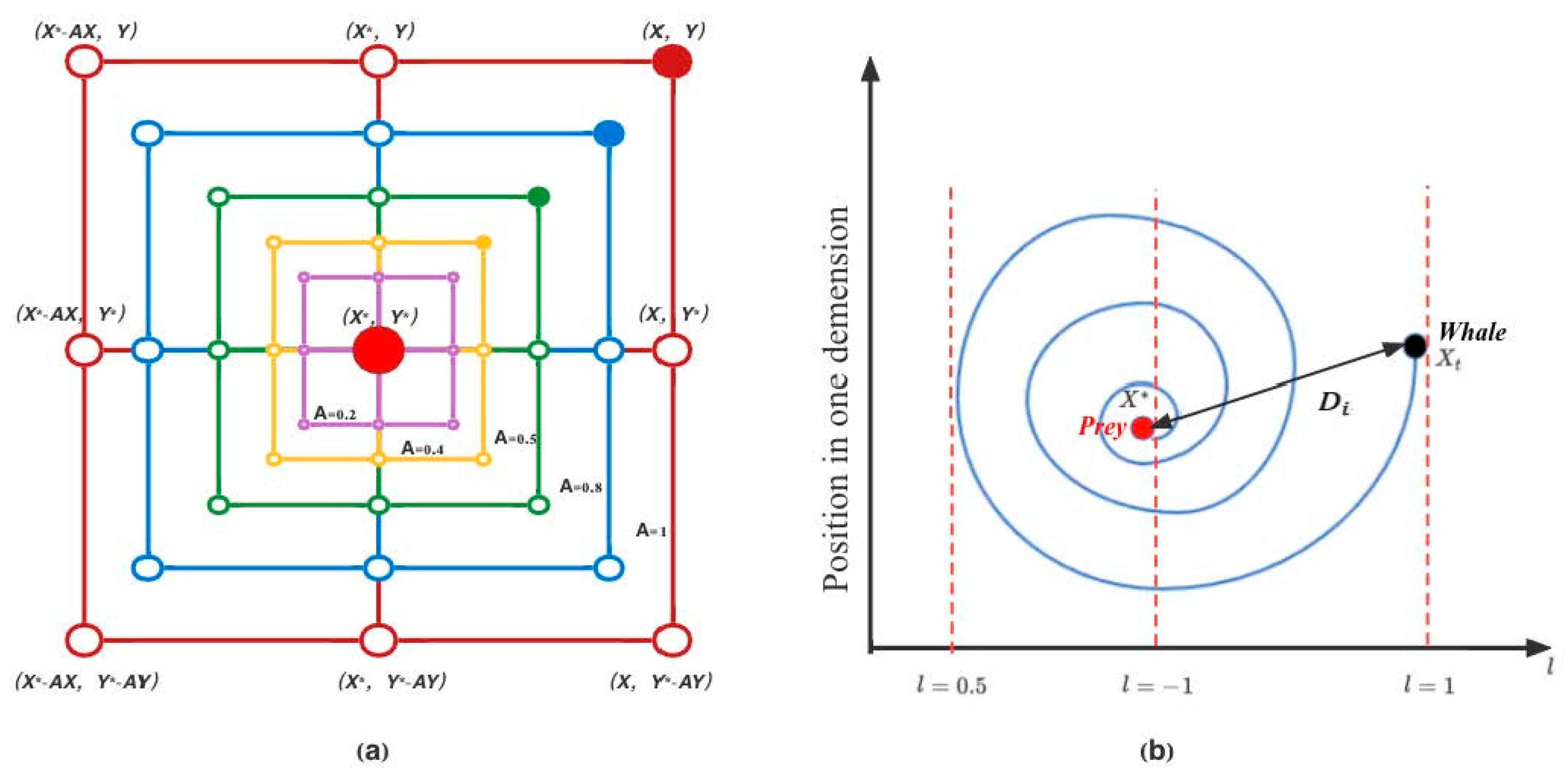
3.2.1. Exploitation Phase (Encircling Prey/Bubble-Net Attacking Method)

Mirjalili et al. designed two methods to mathematically model the bubble-net behavior of humpback whale, one of which is the shrinking encircling mechanism and the other is the spiral updating position. We then analyze the concrete implementation of these two processes from a mathematical point of view.

In the shrinking encircling mechanism, WOA applies the following two formulas to update the problem solution to model the movement of a whale toward a prey.

$$\overrightarrow{D}=\left|\overrightarrow{C.}\overrightarrow{X^{*}}\left(t\right)-\overrightarrow{X}\left(t\right)\right|$$

(1)

$$\overrightarrow{X}\left(t+1\right)=\left|\overrightarrow{X^{*}}\left(t\right)-\overrightarrow{A}.\overrightarrow{D}\right|$$

(2)

where $t$ represents the number of current iterations, $\overrightarrow{X^{*}}$ represents the optimal solution obtained so far, $\overrightarrow{X}$ is the current solution scheme, $|⬚|$ is the absolute value, and $.$ is the dot product operation between the elements. $\overrightarrow{A}$ and $\overrightarrow{C}$ are the coefficient vectors, which can be obtained from Equations (3)–(5):

$$\overrightarrow{A}=2\overrightarrow{a}.\overrightarrow{r}-\overrightarrow{a}$$

(3)

$$\overrightarrow{C}=2.\overrightarrow{r}$$

(4)

$$a=t\frac{2}{MaxIter}$$

(5)

where the value of $A$ decreases linearly from 2 to 0 and its value is in the interval [−$a$, $a$]. $r$ is a random vector between [0, 1]. $a$ increases linearly from 0 to 2 depending on the number of iterations. $t$ is the number of the current iteration, and $Maxiter$ is the maximum number of pre-set iterations.

According to Equation (2), the current solution updates the position of the current solution according to the optimal solution obtained so far. Through the two vectors $A$ and $C$, the search range of the current solution can be controlled to be fixed within the neighborhood range of the optimal solution. In order to imitate the behavior of whales hunting prey in Figure 2b, we use the mathematical model shown in Figure 3a for modeling and analysis. It is assumed that $\left(X^{*},Y^{*}\right)$ is the current global optimal solution, and the solid dots in the figure, such as $\left(X,Y\right)$, are the current solution. Figure 3a shows the possible positions from $\left(X,Y\right)$ toward $\left(X^{*},Y^{*}\right)$ that can be achieved by $0\le A\le 1$ in a 2D space.

As mentioned above, whales also use a spiral motion to move toward prey as shown in Figure 2c. WOA uses the following formula to model this behavior.

$$\overrightarrow{X}\left(t+1\right)=D^{\prime }.e^{bl}.cos\left(2\pi l\right)+\overrightarrow{X^{*}}\left(t\right)$$

(6)

where $\overrightarrow{X^{*}}$ represents the optimal solution obtained so far, $\overrightarrow{X}$ is the current $i\mathrm{th}$ solution, $D^{\prime }$ = |$\overrightarrow{X^{*}}\left(t\right)-\overrightarrow{X}\left(t\right)\vee$ and indicates the distance of the $i\mathrm{th}$ whale to the prey (best solution obtained so far), $b$ is a constant for defining the shape of the spiral, and $l$ is a random variable between [−1, 1].

The approximate figure of Equation (6) and Figure 2c is shown in Figure 3b. In this 1D space, $X_t$ represents the current $i\mathrm{th}$ solution (i.e., the whale), $X^{*}$ represents the current optimal solution (i.e., the prey), and the distance between $X_t$ and $X^{*}$ is $D_i.$ The x-coordinate of the coordinate axis represents a random number $l$, which is used to control the movement direction of the whale, and the y-coordinate represents the next position $X_{\left(t+1\right)}$ of the current solution $X_t$. In order to simulate the behavior of humpback whales swimming around prey while following a spiral-shaped track in a shrinking circle, the authors consider the contraction and spiral rise processes to occur equally with probability, and the mechanism is defined in Equation (7).

$$\overrightarrow{X}\left(t+1\right)=\{\begin{array}{c}\left|\overrightarrow{X^{*}}\left(t\right)-\overrightarrow{A}.\overrightarrow{D}\right|if\left(p<0.5\right)\\ D^{\prime }.e^{bl}.cos\left(2\pi l\right)+\overrightarrow{X^{*}}\left(t\right)if\left(p\ge 0.5\right)\end{array}$$

(7)

where $p$ is a random variable between [0, 1].

3.2.2. Exploration Phase (Search for Prey)

As mentioned above, besides moving toward the lead whale, the whale can also move in a random direction, as shown in Figure 2a. This is called the exploration phase in WOA. In this phase, we no longer require a random search of the solution based on the position of the optimal solution found so far, but instead update the position with randomly selected solutions. Thus, a vector with a random value greater than 1 or less than −1 is used to force a solution away from the optimal search agent. This mechanism can be expressed in mathematical models as Equations (8) and (9).

$$\overrightarrow{D}=\left|\overrightarrow{C.}{\overrightarrow{X}}_{rand}-\overrightarrow{X}\right|$$

(8)

$$\overrightarrow{X}\left(t+1\right)=\left|{\overrightarrow{X}}_{rand}-\overrightarrow{A}.\overrightarrow{D}\right|$$

(9)

where ${\overrightarrow{X}}_{rand}$ is a random solution of the current solution vector set. The meanings of the other notations are mentioned above.

In WOA, the author uses $A$ to control whether the algorithm specifically executes the exploitation phase or exploration phase. When the absolute value of $A$ is greater than 1, WOA chooses to execute the exploration phase; when the absolute value of A is less than 1, WOA chooses to execute the exploitation phase. As mentioned in the previous paper, the value range of $A$ is $\left[-a,a\right]$, and the value of $A$ decreases linearly with the increase in the number of iterations. Therefore, in the general trend, WOA has more chances to jump out of the current optimal solution and choose the random solution at the early stage of implementation. With the increase in the number of iterations, the range of $A$ will gradually shrink, and the WOA will gradually converge to the optimal solution.

4. Proposed Method

In this section, we introduce our proposed algorithm in detail. First, in Section 4.1, we introduce two different coding schemes corresponding to the local and global versions of the WOA applied to hierarchical clustering. In Section 4.2, we describe the fitness function that generates alarm clustering using the WOA. In Section 4.3, we combine the WOA with the crossover and variation factors of the genetic algorithm and propose the pseudo-codes of the local and global versions of the WOA alarm hierarchical clustering algorithm.

4.1. Encoding and Decoding

We first introduced the encoding and decoding scheme of the local version of the WOA applied to hierarchical clustering. In this scheme, a search agent in the WOA corresponds to a cluster center of hierarchical clustering. As mentioned above, a cluster center is composed of a basic alarm or an abstract alarm, so we can obtain the data structure encoded by the search agent. Each attribute in the alarm corresponds to a binary string in the encoded data structure, represented by 0 or 1, as shown in Figure 4.

Figure 5a shows the coding scheme of the cluster center in binary form, and Figure 5b shows the attribute values of the cluster center corresponding to this coding. Figure 4 shows an alarm with four attributes (A, B, C, and D) with decimal values of 3, 6, 1, and 5. The four attribute fields of the alarm are located in their respective hierarchical trees, as shown in Figure 5.

We can find the location of the node corresponding to the binary-encoded attribute in the hierarchical tree. At the same time, we can easily obtain the binary fragment corresponding to the alarm through the hierarchical tree. This coding scheme indicates that a search agent corresponds to a cluster center. The goal of the WOA is to find the best search agent for the fitness function over multiple iterations, output its corresponding cluster center, and categorize the alarms that belong to that cluster.

In this encoding and decoding scheme, a WOA search agent corresponds to a cluster center, assuming that the cluster center is composed of $N$ attributes and the binary length of each attribute is $K$, then the encoding length of a search agent is $N\ast K$, corresponding to $N$ hierarchical trees.

After giving the encoding and decoding scheme of the local version WOA–hierarchical tree, we introduce the encoding and decoding schemes of the global version WOA–hierarchical tree. In the coding scheme of the global version, a WOA search agent is composed of a group of cluster centers. Assuming that WOA eventually obtains $C$ cluster centers, each of which is composed of $N$ attributes with length $K$, the coding length of the global version WOA–hierarchical tree is $C\ast N\ast K$. Let us take the example shown in Figure 6 for illustration.

In Figure 6, there are three hierarchical trees corresponding to the three attributes of an alarm, respectively. If we need to finally obtain three cluster centers for this alarm set, which are $\left(\mathrm{A}4,\mathrm{B}2,\mathrm{C}3\right)$, $\left(\mathrm{A}1,\mathrm{B}1,\mathrm{C}2\right)$ and $\left(\mathrm{A}3,\mathrm{B}2,\mathrm{C}4\right)$, then one of our search agents can be encoded as shown in Figure 7a in the second coding method. Figure 7b shows the three cluster centers corresponding to this coding scheme.

4.2. Fitness Function

The core of WOA is to find the best solution set in a finite solution set space through a finite number of iterations. The fitness function is the standard to evaluate whether a solution set is excellent. Therefore, how to set up an appropriate fitness function is the key to solve the problem of hierarchical clustering using WOA. The selection of the fitness function in this paper mainly considers the following three factors: the number of alarms contained in the cluster center, the distance between alarms belonging to the same cluster, and the coincidence degree between clusters. We believe that, given a fixed threshold of alarm distance, the more alarms that a cluster contains, the greater the fitness value will be. In addition, when the similarity of alarms belonging to the same cluster is higher (the distance is smaller), the fitness value is higher. If the coincidence degree of cluster center is higher, we believe that the meanings of the two clusters are closer, and the overall fitness value will be smaller.

For a given alarm cluster center, $S=\left(N_1,N_2,N_{3,}{N}_4,\dots N_m\right)$, where the value of m corresponds to the number of hierarchical trees used in the alarm cluster. If the alarm distance meets the number of alarms within the given threshold, we believe that the fitness of the alarm cluster center is higher. In Refs. [45,46,47], the setting of the fitness function is to determine whether the number of alarms belonging to a certain alarm cluster center exceeds the given threshold. If the number exceeds, the fitness is set to 1, and if not, the fitness is set to 0. This processing method has a simple idea and can well distinguish the alarms that do not meet the clustering requirements from those that meet the clustering requirements. However, the problem is that the method cannot reflect the quality of the cluster centers which exceed the threshold value. For example, if the threshold value is set to 500, the existing two clusters $C_1$ and $C_2$ contain alarm numbers of 2000 and 5000, respectively. We intuitively feel that $C_2$ is better than $C_1$ but their fitness values are set to the same value, which does not achieve a good distinction. In this paper, a new calculation method of alarm number fitness is adopted, as shown in Equation (10).

$$E_{T}k\left(t,x\right)=\{\begin{array}{c}0,if\left(x<t\right)\\ ln\left(\frac{x}{t}\right),if\left(x\ge t\right)\end{array}$$

(10)

where $t$ represents the threshold of the number of alarms that the cluster should contain, and $x$ represents the number of alarms belong to the cluster center.

When $x<t$, we think that the cluster contains too few alarms, and the cluster center should not be selected; when $x>t$, we think that the fitness value of the cluster center increases with the increase in $x$, and taking $t=500$ as an example, the image of the fitness function is shown in Figure 8.

For a cluster center, only considering the number of alarms contained in the cluster center as an evaluation index cannot indicate the quality of the cluster center. Only when the number of alarms contained in the cluster center is large enough and the difference between alarms is small enough do we believe that the selection of the cluster center is reasonable. Therefore, we define a fitness function for the internal differences in the alarm cluster center, as shown in Equation (11). The average depth of the four hierarchical trees as shown in Figure 1 is (3 + 2 + 3 + 2)/4 = 2.5.

$$E_S\left(k\right)=\frac{1}{n}{\displaystyle \sum }_{i=1}^n\left(1-\frac{D\left(C_i\right)}{M_d}\right)$$

(11)

where $i=\left(1,2,3,\dots ,n\right)$ represents $n$ alarms belonging to a cluster center k, $D\left(C_i\right)$ represents the sum of the distances between the alarm and each attribute of the cluster center in its attribute tree, and $M_d$ represents the average depth of all attribute hierarchy trees.

4.3. Crossover and Mutation Operator

One of the difficulties of the WOA in solving hierarchical clustering problems is how to apply Equations (2), (6) and (9) to transform search agent positions for different types of attributes. If an attribute is a continuous variable, the use of the above formula is not affected, but if an attribute is a discrete variable then using the formula is difficult. Because we use the attributes of the hierarchical tree structure and type of binary coding structure, we can easily transform the attributes into a hierarchical tree. Here, we use crossover and mutation operators of the genetic algorithm to solve this problem. Another advantage of using these two operators is that the WOA is combined with crossover and genetic operators to further improve the algorithm’s ability to search for local and global optimal solutions. This conclusion is mentioned in Ref. [48].

Now, we present the application of crossover operator based on the WOA coding scheme. Taking an alarm with four attributes as an example, the binary identity of the attribute field with two alarms is shown in Figure 9.

As can be seen from Figure 10, the attributes of the two coded alarms are $Alarm1 \left(A_3{B}_6{C}_1{D}_5\right)$ and $Alarm2 \left(A_3{B}_{10}{C}_2{D}_3\right).$ Starting with 6 bit, cross transposition of the attributes of the two alarms can be carried out so that two new alarms can be obtained after operation, as shown in Figure 10.

From Figure 10, we can see that the two new alarms, $Alarm{1}^{\prime } \left(A_3{B}_6{C}_2{D}_3\right)$ and $Alarm{2}^{\prime } \left(A_3{B}_{10}{C}_1{D}_5\right)$, are generated after crossing. Looking at the changes in the attribute fields of the two alarms, we find that, except for the change in the attribute of the exchange location, the other attributes only changed the location.

After introducing the application of crossover operator in alarm clustering, we introduce the use of the mutation operator in alarm clustering. Taking the alarm shown in the left figure of Figure 9 as an example, the change of the alarm after a mutation operation is performed on a bit of the alarm attribute is shown in the right figure of Figure 11. By changing the value of the sixth bit in the binary from 1 to 0, the alarm changes from $Alarm \left(A_1,B_5,C_6\right)$ to $Alar{m}^{⬚}\left(A_1,B_4,C_6\right)$. Observing the change in the alarm, we can find that the mutation operation only makes a certain attribute of the alarm field change, while the other attributes remain unchanged.

4.4. WOA-Based Alarm Hierarchical Clustering Process

After introducing the coding and decoding scheme, fitness function and crossover and mutation operator of the WOA applied to hierarchical clustering, in this section, we present the processing of the local and global versions of WOA applied to the alarm hierarchical clustering process. In order to express clearly, the WOA hierarchical clustering of the local version and global version are respectively called WOAHC-L and WOAHC-G. Compared with the traditional alarm hierarchical clustering algorithm, which can only generate one random generalization alarm at a time, WOA uses multiple search agents to search the solution set space of the generalization alarm simultaneously, which can improve efficiency and obtain more possibilities of solution sets. The random agent selection stage of WOA provides a higher possibility to jump out of the local optimum to find a better solution set. The use of crossover operators and mutation operators can help WOA deal with various types of data and enhance the ability of local search and global search.

We first provide the algorithm flow of WOAHC-L. The process of WOAHC-L can be described as follows: the algorithm first initializes several search agents, each representing a cluster center of the alarm. Then, we calculate the fitness value of each search agent according to the fitness function. The cluster center represented by the search agent with the best fitness value is the optimal solution. After that, according to WOA’s search mechanism, the remaining search agents explore the solution set space around the optimal solution through exploitation phase and exploration phase and update the value of the optimal solution whenever there is a better solution. After several iterations, the cluster center represented by the search agent with the optimal fitness value is output, and alarms belonging to that cluster are added to the cluster and removed from the original alarm set. Each time the algorithm is executed, a cluster center is output and the alarms belonging to the cluster are deleted from the original alarm set. When the remaining alarms no longer meet the clustering rules after several times of algorithm execution, the algorithm is finished. The alarm clustering process based on WOAHC-L is shown in Figure 12.

The algorithm pseudocode of WOAHC-L is shown in Algorithm 2.

Algorithm 2 WOA for alarm hierarchical clustering (local version)

Input: threshold, N, maxIteration, mutation rate, t = 0, k = 0 Output: alarm_center[], alarms after clustering 1: while the number of current alarms is bigger than threshold do 2:   Randomly generate initial population Xi (i = 1, 2, …, N) 3:   Calculate the fitness value of each solution 4:   Get the best Xi that has the largest fitness value, mark it as X* 5:   while t < MaxIterationr do 6:     for population Xi(i = 1, 2, …, N) do 7:      Use Equations (3)–(5) to update a,A,C 8:      Generate values for random numbers 1 and P 9:      if p < 0.5 then 10:       if |A| < 1 then 11:        Use Equations (1) and (2) to update the position of Xi 12:        Apply mutation operation on X* (best solution) given mutation rate (r) to get Xmut 13:        Perform crossover operation between Xmut and Xi 14:        Set the new position of Xi to the output of crossover operation 15:       else if |A| ≥ 1 then 16:        Select a random search agent (Xrand) 17:        Use Equations (8) and (9) to update the position of Xi 18:        Apply mutation operation on Xrand given mutation rate(r) to get Xmut 19:        Perform crossover operation between Xmut and Xrand 20:        Set the new position of Xi to the output of crossover operation 21:       end if 22:      else if p ≥ 0.5 then 23:       Use Equation (6) to update the position of the current solution Xi 24:       Apply mutation operation on X* (best solution) given mutation rate (r) to get Xmut 25:       Perform crossover operation between Xmut and Xi 26:       Set the new Position of Xi to the output of crossover operation 27:      end if 28:     end for 29:     Calculate the ftness value of each solution, check if any solution goes beyond the search space 30:     If there is a better solution Xi update Xi as X* 31:     t = t + 1 32:   end while 33:   Mark X* as cluster k 34:   Put alarms which belong to the cluster k to the alarm_center[k] 35:   Remove alarms from the original alarms set 36:   k = k + 1 37: end while

Based on the excellent local and global search capabilities and the group search mechanism of WOAHC-L algorithm, we can find excellent alarm cluster centers. However, the problem of WOAHC-L is that there may be a high degree of overlap between the cluster centers obtained by executing WOAHC-L several times, so that the alarm sets originally belonging to the same cluster may be divided into multiple clusters. In other words, WOAHC-L only focuses on the generation of single cluster centers and does not consider the overlap between the finally obtained cluster centers. In order to solve the above problem of the WOAHC-L algorithm, we propose a global version based on WOA hierarchical clustering, namely WOAHC-G, which uses the second encoding scheme of the search agent mentioned in Section 4.1 above.

The process of WOAHC-G can be described as follows: the algorithm initializes several search agents, each of which is composed of $N$ cluster centers and represents the final clustering result. According to the fitness function, each search agent calculates a fitness value. The search agent with the best fitness value is the optimal search agent, and the cluster center represented by the agent is the final cluster center set. Based on the WOA exploitation phase and exploration phase, the cluster center set represented by the search agent with the optimal fitness value is finally obtained after several iterations. WOAHC-G differs from WOAHC-L in that WOAHC-G only needs to execute once to obtain all cluster centers, while WOAHC-L needs to execute several times until the number of remaining alarms is insufficient for the next algorithm execution. In addition, WOAHC-G considers the problem of coincidence degree between different cluster centers and takes the coincidence degree as an important indicator of fitness value. Therefore, the fitness function of the algorithm needs to be changed to add the coincidence degree of cluster centers, as shown in Equation (12).

$$\mathit{O}\left({\mathit{C}}_{\mathit{i}},{\mathit{C}}_{\mathit{j}}\right)=\{\begin{array}{c}\mathbf{1},{\mathit{C}}_{\mathit{i}}{{\displaystyle \cap }}^{}{\mathit{C}}_{\mathit{j}}=\varnothing \\ \mathbf{0},{\mathit{C}}_{\mathit{i}}{{\displaystyle \cap }}^{}{\mathit{C}}_{\mathit{j}}\ne \varnothing \end{array}$$

(12)

where ${\mathit{C}}_{\mathit{i}},{\mathit{C}}_{\mathit{j}}$ represent two cluster centers. If each attribute of the two cluster centers has no intersection, the coincidence degree is considered to be 0; otherwise, it is 1.

After the calculation function of clustering coincidence degree is given, the evaluation equation of clustering coincidence degree is given as Equation (13).

$$E{S}_o=\frac{2}{k\left(k-1\right)}{\displaystyle \sum }_{0\le i<j\le k}O\left(C_i,C_j\right)$$

(13)

where $k$ represents the number of cluster centers. When there are $k$ cluster centers, $\frac{k\left(k-1\right)}{2}$ times are needed to calculate the coincidence degree between them. Therefore, the coefficient in the calculation formula of $E{S}_o$ is set as $\frac{2}{k\left(k-1\right)}$ to ensure that the value of $E{S}_o$ is within the interval [0, 1].

The alarm clustering process based on WOAHC-G is shown in Figure 13.

The algorithm pseudocode of WOAHC-G is shown in Algorithm 3

Algorithm 3 WOA for alarm hierarchical clustering (global version)

Input: N, maxIteration, mutation rate, t = 0, k = 0 Output: alarm_center[], alarms after clustering  1: Randomly generate initial population Xi (i = 1, 2, …, N)  2: Calculate the fitness value of each solution  3: Get the best Xi that has the largest fitness value, mark it as X*  4: while t < MaxIteration do  5:   for population Xi (i = 1, 2, …, N) do  6:    Use Equations (3)–(5) to update a,A,C  7:    Generate values for random numbers 1 and p  8:    if p < 0.5 then  9:     if |A| < 1 then  10:      Use Equations (1) and (2) to update the position of Xi  11:      Apply mutation operation on X* (best solution) given mutation rate (r) to get Xmut  12:      Perform crossover operation between Xmut and Xi  13:      Set the new position of Xi to the output of crossover operation  14:     else if |A| ≥ 1 then  15:      Select a random search agent (Xrand)  16:      Use Equations (8) and (9) to update the position of Xi  17:      Apply mutation operation on Xrand given mutation rate (r) to get Xmut  18:      Perform crossover operation between Xmut and Xrand  19:      Set the new position of Xi to the output of crossover operation  20:     end if  21;    else if p ≥ 0.5 then  22:     Use Equation (6) to update the position of the current solution Xi  23:     Apply mutation operation on X* (best solution) given mutation rate (r) to get Xmut  24:     Perform crossover operation between Xmut and Xi  25:     Set the new position of Xi to the output of crossover operation  26:   end if  27:   end for  28:   Calculate the fitness of each solution, check if any solution goes beyond the search space  29:   If there is a better solution Xi, update Xi as X*  30:   t = t + 1  31 end while  32: return X*

5. Experiments and Results

5.1. Experiment Data Set

In this section we describe the data sets used in the experiment. We use UNSW-NB15 as the experimental data set [8]. The UNSW-NB15 data set was developed by Ixia Perfectstorm. It is used to simulate and generate real and contemporary attack models. This is a tool called Tcpdump, which contains up to 100 GB of PCAP files and is used to simulate nine different types of attacks. These include DOS, Shellcode, worms, Fuzzers, backdoors, exploits, analytics, generality, and scouts. In addition, the data set consists of 12 algorithms for generating 49 features belonging to class tags. The following

Table 2. UNSW-NB15 Features with their data type and category.

Category	No	Name	Data Type	Category	No	Name	Data Type
Flow	1	srcip	Nominal	Content	25	trans_depth	Integer
	2	sport	Integer		26	res_bdy_len	Integer
	3	dstip	Nominal	Time	27	Sjit	Float
	4	dsport	Integer		28	Djit	Float
	5	proto	Nominal		29	Stime	Timestamp
Basic	6	state	Nominal		30	Ltime	Timestamp
	7	dur	Float		31	Sintpkt	Float
	8	sbytes	Integer		32	Dintpkt	Float
	9	dbytes	Integer		33	Tcprtt	Float
	10	sttl	Integer		34	Synacj	Float
	11	dttl	Integer		35	Ackdat	Float
	12	sloss	Integer	General	36	Is_sm_ips_ports	Binary
	13	dloss	Integer	Purpose	37	Ct_state_ttl	Integer
	14	service	Nominal		38	Ct_flw_http_mthd	Integer
	15	Sload	Float		39	Is_ftp_login	Binary
	16	Dload	Float		40	Ct_ftp_cmd	Integer
	17	Spkts	Integer	Connection	41	Ct_srv_src	Integer
	18	Dpkts	Integer		42	Ct_srv_dst	Integer
Content	19	swin	Integer		43	Ct_dst_ltm	Integer
	20	dwin	Integer		44	Ct_src_ltm	Integer
	21	stcpb	Integer		45	Ct_src_dport_ltm	Integer
	22	dtcpb	Integer		46	Ct_dst_sport_ltm	Integer
	23	smeansz	Integer		47	Ct_dst_src_ltm	Integer
	24	dmeansz	Integer		48	Attack_cat	Nominal
					49	Class	Binary

shows a set of features in UNSW-NB15, along with the corresponding groups and data types.

The UNSW-NB15 data set has a total of 2,540,044 records, which are stored in four files respectively. In order to better conduct the experiment, the data set provides the training set and test set that have removed the missing values, with 175,341 records and 82,332 records respectively. As can be seen from the above table, the 49 fields in the data set include fields of different types, such as Flow, Basic, Content, Time, Content, etc., and each attribute belongs to either the discrete or continuous types.

5.2. Experimental Setup

The experimental operating environment used Intel Core i5-7500CPU 3.40 GHz and 8 GB memory. The configuration of the software environment is as follows: the operating system is Microsoft Windows 10, the experimental program is written in Python, and the development version is Python 3.7.3. We use PyCharm and Juptyer Notebook as the integrated development environment for Python. In addition, we use WEKA as an auxiliary tool for data processing and analysis. WEKA is an open-source machine learning and data mining software based on Java environment [49]. It is one of the most complete data mining tools today.

5.3. Experimental Results

As mentioned above, we use the UNSW-NB15 data set as our experimental data set. A total of 50,801 data were randomly selected from the training set and test set to carry out the clustering calculation of the alarm. The extracted alarm label distribution is shown in

Table 3. Distribution of alarm labels in 50,801 pieces of data.

	Attack_Catgory	Number		Attack_Catgory	Number
1	Null	44,387	6	Reconnaissance	289
2	Generic	4257	7	Backdoor	53
3	Exploits	913	8	Analysis	52
4	Fizzers	463	9	Shellcode	29
5	DoS	355	10	Worms	3

.

Attack types marked 2–10 in the table represent specific types of attacks, while the type marked 1 is normal network traffic. It is not difficult to see that this data set contains a large number of normal network traffic, which is identified by IDS as a malicious alarm, resulting in a large number of false alarms. Our goal is to use clustering methods to correctly identify normal network traffic and eliminate it from alarms.

We analyze the source IP address and destination IP address in the experimental data set as follows. The data set contains two types of IP addresses: Class B and Class C (such as Class C IP addresses 149.171.126.43 and 149.171.126.50). We can extract the same fields and classify the IP addresses, and the uncertain part is represented by X. The statistics of each type of IP address and its number are shown in

Table 4. Distribution of source and destination IP addresses.

Source_IP	Number	Destination_IP	Number
59.166.0.X	38,817	149.171.126	46,051
175.45.176.X	7234	175.45.176	4284
149.171.126.X	4338	10.40.X.X	298
10.40.X.X	412	224.0.0.X	108
		59.166.0.X	55
		192.168.241	5

.

After analyzing the experimental data, we first explore the performance of WOAHC-L in looking for a single alarm cluster center. The specific parameters of WOAHC-L are set as follows: $SearchAgents$ = 10 and $MaxIter$ = 50, respectively, which means that we use 10 search agents to search the solution space of the clustering at the same time, and the maximum number of iterations of the algorithm is 50. Other parameters in WOAHC-L, such as $r,a,p$, etc., are generated by random numbers or are related to $MaxIter$ so we do not have to set it up. The fitness function is set as the equation mentioned in Section 4.2.

According to the mechanism of WOAHC-L, the cluster center obtained by calling the algorithm for the first time has the best fitness value. In order to explore the performance of WOA in hierarchical clustering, we independently perform WOAHC-L four times and record the change in the optimal fitness value with the number of iterations during each algorithm execution. The performance of WOAHC-L is shown in Figure 14. The X axis is the number of iterations and the Y axis is the fitness value of the currently found optimal cluster center.

As can be seen from Figure 14, WOAHC-L constantly seeks the most excellent cluster center in the search space through its exploitation phase and exploration phase. It can be seen from the figure that WOAHC-L has an excellent ability to break through the local optimum, which can be clearly seen from the stage of 20–50 iteration times.

After verifying that WOAHC-L has excellent global search capability in alarm clustering, we continue to explore the use of WOAHC-L to solve the local clustering problem of alarm hierarchical clustering, that is, every time we call the WOAHC-L, an alarm cluster is obtained, which is obtained through the iterative search of WOAHC-L, according to the fitness function. Taking $MaxIter$ of 50 as the maximum number of iterations and the number of search agents of 10 as an example, we perform WOAHC-L four times and obtain four cluster centers successively from 50,801 alarms. The number of alarms contained in the four cluster centers varies with the number of iterations as shown in Figure 15.

According to the experimental statistics, the number of alarms contained in each cluster obtained by calling WOAHC-L four times is as follows. By analyzing the obtained cluster center, we find that the tag field in the cluster center obtained by the first, second and fourth calls to WOAHC-L is $\left(null,0\right)$, and the tag field in the cluster center obtained by the third calls to WOAHC-L is $\left(Generic,1\right)$. In other words, these four calls to WOAHC-L distinguish the generic attacks from the normal traffic in the original data set by clustering. We add up the number of alarms generated by the first, second and fourth calls to WOA to 45,469, which is within the allowable range when compared with the number of normal network traffic 44,387 in the table. The third call to the WOAHC-L cluster is 3819, which is within an acceptable distance of the 4257 alarms for the generic attacks in the table. This experiment proves that hierarchical clustering using WOAHC-L can well distinguish the type of alarm.

After proving WOAHC-L’s excellent local and global search ability and clustering ability, we next explore statistical analysis of WOAHC-L on time consumption and clustering results. Based on the algorithm flow of WOAHC-L in Figure 12, when the number of remaining alarms no longer meets the clustering threshold, the algorithm ends, and the clustering result is output. Therefore, we constantly call WOAHC-L to obtain new clustering until the condition of the algorithm ending is met. The experimental results are shown in Figure 16.

As can be seen from Figure 16, as the number of algorithm executions increases, the time of each algorithm execution gradually decreases, and the number of alarms contained in the cluster obtained by each invocation of the algorithm also decreases. The reason is obviously that every time the algorithm is called to obtain the cluster center, the alarms belonging to the cluster in the alarm set are removed from the alarm set, so the next time the algorithm is called, the alarm items scanned by the algorithm are fewer and fewer, and the time and number of alarms are also reduced.

In order to verify the robustness of WOAHC-L, we conduct five experiments. In each experiment, WOAHC-L is called several times to obtain multiple cluster centers, until the amount of remaining data in the data set are less than the requirement of alarm clustering.

As can be seen from

Table 5. The results of the number of alarms contained in the cluster and the number of algorithms calls in five experiments.

Time Rounds	1	2	3	4	5	6	7	8	9	10	11	Time Consuming
1	18,433	14,870	3219	6553	4170	745	421	921	31	29	51	66.3 s
2	38,923	4331	3490	993	671	210	78	32				52.0 s
3	36,544	4370	4921	2008	719	198	43	23	104	97		56.5 s
4	24,003	18,995	4109	529	899	32	390	241	45	122		55.3 s
5	15,023	30,901	2104	2233	920	320	429	290	102			63.4 s

, except the first row, there are five rows in the table, representing five experiments. Except the first column, from a total of 12 columns, the top 11 columns represent each experiment that invokes the WOAHC-L to obtain cluster center containing the number of alarms. What we need to pay attention to is that in the table there are some gaps, such as the third line 10 columns; these blanks show that the experiments, after several WOAHC-L calls, have met the conditions of the end of the algorithm, such as the second experiment. We find that WOAHC-L is called eight times and then stops executing. The last column of the table represents the total time of the experiment. Compared with the five experiments, the average time and standard deviation of the total time spent in our calculation algorithm are 58.7 s and 5.3, which are within the allowable range of the experiment. In addition, we should also note that although the number of cluster centers generated by each experiment is different (the five experiments are 11, 8, 10, 10, and 9, respectively), as we mentioned before, cluster centers generated by this kind of local clustering method will cause the problem of a too high coincidence degree of cluster centers. However, we can study the experimental data in the first experiment of two previous cluster centers containing the sum of the number of alarms for 33,303. For the properties of alarm analysis, we find that they all belong to the normal network traffic, so we can combine the two-cluster center as a cluster center, representing the clustering of normal network traffic. Excluding the problem of clustering overlap, we have reason to believe that the robustness of the algorithm is relatively excellent.

Meanwhile, in order to compare with other algorithms, we repeat the alarm clustering algorithm mentioned in the references [45,46,47] and compare it with WOAHC-L. In order to more intuitively feel the results of clustering, we use the number of alarms contained in the cluster center as the Y axis to compare the four algorithms. Please note that it is not accurate to rely only on the number of clusters contained in the cluster center to evaluate the quality of the clustering results. The quality of the clustering results is also greatly related to the distance between the alerts contained in the cluster center (called difference in some works), that is, the fitness function mentioned in the formula. The experimental results are shown in Figure 17.

As can be seen from Figure 17, compared with Julisch’s algorithm, SA and GA, WOAHC-L can well jump out of the local optimum in the process of clustering search, while other algorithms begin to converge at the beginning or middle of the iteration and no longer search for a better cluster center. We need to emphasize that the purpose of this experiment is to intuitively show that compared with the other three algorithms, WOAHC-L can better jump out of the local optimal and achieve better results when carrying out hierarchical clustering. A more detailed comparison of experimental results with other algorithms is presented in the following experiments. We use the following formula to calculate the values of these indicators.

$$Accuracy=\frac{TP+TN}{TP+FP+TN+FN}$$

(14)

$$Precision=\frac{TP}{TP+FP}$$

(15)

$$Recall=\frac{TP}{TP+FN}$$

(16)

where $TP$ represents the number of normal network traffic clustering to normal cluster, $TN$ represents the number of network attack clustering to attack cluster, $FP$ represents the number of network attack alarms incorrectly clustering to normal cluster, $FN$ represents the number of normal network traffic incorrectly clustering to the attack cluster. $Accuracy$ represents the accuracy of the clustering; $Precision$ represents how much of the data clustered as normal traffic are really normal traffic; and $Recall$ represents how much of the normal traffic is correctly clustered.

Table 6. A detailed comparison of experimental results between WOA and Julisch’s method, GA and SA.

	Cluster Numbers	Time Consuming	Remaining Alarms	Accuracy	Precision	Recall
Julisch’s method	16	43.2	831.4	91.8%	97.6%	92.9%
GA-based	10	31.5	432.4	93.5%	97.1%	95.4%
SA-based	13	25.5	913.0	91.7%	96.7%	93.7%
WOAHC-L	10	68.3	322.5	95.2%	98.4%	96.1%

shows the comparison of various indicators of different algorithms. These indicators have specific meanings, introduced in Table 1.

As can be seen from Table 6, WOAHC-L is obviously superior to other algorithms in terms of the number of clustering, number of remaining alarms, accuracy, precision and recall. It should be noted that recall refers to the rate of aggregation of false alarms, or reduction in redundant alarms. However, WOAHC-L has obvious deficiencies in terms of time consumption, which is caused by the multi-search agent mechanism of the WOA and the calculation of the fitness value.

As the excellent performance of WOAHC-L in alarm reduction is proved by comparing with other algorithms, we explore the stability of WOAHC-L in clustering and the rule analysis of clustering results. In order to avoid the contingency of experimental results, we conduct eight experiments, where each experiment performs several WOAHC-L times until the number of remaining alarms no longer meets the clustering requirements. The results of the experiment are shown in Figure 18. The X axis represents the number of cluster centers, that is, the number of WOAHC-L calls, and the Y axis represents the number of remaining alarms in the original alarm set.

According to Figure 18, we find that in the eight experiments, WOAHC-L generates cluster centers with more alarms in the previous calls. According to the output of the code, we can find that these cluster centers are all clusters related to redundant alarms, which is consistent with our expected assumption: WOAHC-L first clusters redundant false alarms that account for a higher proportion in the alarm data set, and then clusters the remaining real alarms. We set the alarm number threshold of algorithm end condition as 500 and observe that the times of calling WOAHC-L are different in the eight groups of experiments (10, 6, 10, 7, 8, 6, 10, and 7, respectively). In Section 4.4, we explained the reason for this, that is, there may be an overlap between the cluster centers generated by WOAHC-L, and it is confirmed in our experiment.

Through a series of experiments above, we prove the superiority of WOAHC-L in the process of alarm reduction, but its disadvantages are also exposed: the algorithm is time consuming, the results obtained by multiple executions of the algorithm have certain differences (also known as idempotency), and the high degree of overlap between some cluster centers lead to an increase in algorithm calls. To solve this problem, we propose a global clustering version of WOAHC, namely WOAHC-G, and explore the performance of WOAHC-G in the following experiments.

As mentioned in Section 4.4, WOAHC-G only needs to be called once to obtain all the cluster centers, provided that the number of cluster centers need to be specified, which is a difficult problem. However, with the experimental results of WOAHC-L as a reference, we can choose an appropriate number of cluster centers as a parameter. Here, we set the number of cluster centers as eight, which is based on the above experimental results of the comprehensive consideration. Meanwhile, our search agent code is 72 dimensions (each cluster center contains nine attributes, a total of eight cluster centers). We still select 10 search agents to search for the cluster space. Other parameters of WOAHC-G are set as above, and the fitness function of the global version is selected, adding the influence of clustering coincidence degree. Under the same data set configuration, we conduct eight experiments and use a boxplot to represent the number of alarms in each cluster, as shown in Figure 19.

In each boxplot in Figure 19, the blue line at the top represents the maximum, the blue line at the bottom represents the minimum, the upper edge of the square represents the upper quartile, the lower edge represents the lower quartile, the red line represents the median, the green dot represents the average, and the white dots represent outliers. As can be seen from Figure 19, when we fix the number of clustering as 8, the experimental results generated by the eight experiments are basically not significantly different. As can be seen from the number of alarms in cluster 1 to cluster 3, the global clustering version using WOAHC-G can effectively eliminate the problem of excessive cluster repetition. However, the problem of the global clustering version is that it is difficult to determine an appropriate number of cluster centers. In this round of experiments, we set the number of cluster centers to 8 according to the experience of WOAHC-L to eliminate the impact of this problem. However, how to determine an appropriate number of cluster centers requires further research and analysis in the future.

Finally, we discuss the time complexity of the proposed algorithm framework. It is assumed that WOAHC eventually generates $C$ clusters, with a total of $M$ alarms to be clustered, the maximum iteration time of the algorithm is $T$, there are $N$ search agents searching the solution set space at the same time, and each hierarchical tree has $m$ nodes. For WOAHC-L, the time complexity of calculating the fitness value is $O\left(M+lo{g}_{2}m\right)$, so the total time complexity of the algorithm is $O\left(C\ast T\ast N\ast \left(M+lo{g}_{2}m\right)\right)$. During our experiment, $N$ threads are used to search $N$ search agents at the same time, so the time complexity can be optimized to $O\left(C\ast T\ast \left(M+lo{g}_{2}m\right)\right)$. For WOAHC-G, the time complexity of calculating the fitness value is $O\left(lo{g}_{2}m+M+C^2\right)$, so the overall time complexity is $O\left(T\ast N\ast \left(lo{g}_{2}m+M+C^2\right)\right)$, and the time complexity after multithreading optimization is $O\left(T\ast \left(lo{g}_{2}m+M+C^2\right)\right)$.

6. Conclusions and Future Work

In previous studies, in order to solve the problem of a large number of redundant alarms generated by IDS, some scholars proposed the hierarchical alarm clustering algorithm. With the development of the swarm intelligence optimization algorithm, the WOA has been widely used to solve various optimization problems. In this paper, we propose two new methods to solve the problem of alarm reduction by applying the WOA to hierarchical clustering, namely WOAHC-L and WOAHC-G. Through experiments on the UNSW-NB data set, we prove that WOAHC-L can solve the problems of the clustering falling into the local optimum and the poor clustering quality well. Experimental results show that WOAHC-L can achieve 95.2% clustering accuracy and reduce redundant alarms by 96.1%. Compared with WOAHC-L, which generates more than 11 clusters, WOAHC-G reduces the problem of clustering overlap by generating 8 accurate clusters.

Although our new method achieves good results in dealing with redundant alarms, it still has some limitations. For example, WOAHC-L can solve the problem of premature convergence in the clustering process well, but it is easy to produce an excessive number of repeated clusters. WOAHC-G solves this problem well, but it requires the space size of multiple orders of magnitude to encode the hierarchical tree. Meanwhile, WOAHC-G requires a prior number of clusters to ensure that the clustering is not repeated, which will make it difficult to deal with real network problems.

Future work will consider shifting the focus of work to the processing of security events in the real network environment and studying how to adjust a more excellent fitness function to obtain more accurate clustering. In addition, the adaptive setting of the clustering number of WOAHC-G will also be a key point of future work.

References

1. Sun, J.; Gu, L.; Chen, K. An Efficient Alert Aggregation Method Based on Conditional Rough Entropy and Knowledge Granularity. Entropy 2020, 22, 324. [Google Scholar] [CrossRef] [Green Version]
2. Hindy, H.; Brosset, D.; Bayne, E.; Seeam, A.K.; Tachtatzis, C.; Atkinson, R.; Bellekens, X. A taxonomy of network threats and the effect of current datasets on intrusion detection systems. IEEE Access 2020, 8, 104650–104675. [Google Scholar] [CrossRef]
3. Masdari, M.; Khezri, H. A survey and taxonomy of the fuzzy signature-based Intrusion Detection Systems. Appl. Soft Comput. 2020, 92, 106301. [Google Scholar] [CrossRef]
4. Aldweesh, A.; Derhab, A.; Emam, A. Deep learning approaches for anomaly-based intrusion detection systems: A survey, taxonomy, and open issues. Knowl.-Based Syst. 2019, 189, 105124. [Google Scholar] [CrossRef]
5. Siddique, K.; Akhtar, Z.; Khan, F.A.; Kim, Y. KDD Cup 99 Data Sets: A Perspective on the Role of Data Sets in Network Intrusion Detection Research. Computer 2019, 52, 41–51. [Google Scholar] [CrossRef]
6. Ingre, B.; Yadav, A. Performance analysis of NSL-KDD dataset using ANN. In Proceedings of the 2015 International Conference on Signal Processing and Communication Engineering Systems, Guntur, India, 2–3 January 2015; pp. 92–96. [Google Scholar]
7. Alkasassbeh, M.; Al-Naymat, G.; Hassanat, A.B.; Almseidin, M. Detecting Distributed Denial of Service Attacks Using Data Mining Techniques. Int. J. Adv. Comput. Sci. Appl. 2016, 7, 436–445. [Google Scholar] [CrossRef] [Green Version]
8. Moustafa, N.; Slay, J. UNSW-NB15: A comprehensive data set for network intrusion detection systems (UNSW-NB15 network data set). In Proceedings of the 2015 Military Communications and Information Systems Conference (MilCIS), Canberra, ACT, Australia, 10–12 November 2015; pp. 1–6. [Google Scholar]
9. Sharafaldin, I.; Lashkari, A.H.; Ghorbani, A.A. A detailed analysis of the cicids2017 data set. In Proceedings of the International Conference on Information Systems Security and Privacy, Funchal-Madeira, Portuga, 22–24 January 2018; Springer: Cham, Switzerland, 2018; pp. 172–188. [Google Scholar]
10. Damasevicius, R.; Venckauskas, A.; Grigaliunas, S.; Toldinas, J.; Morkevicius, N.; Aleliunas, T.; Smuikys, P. LITNET-2020: An Annotated Real-World Network Flow Dataset for Network Intrusion Detection. Electronics 2020, 9, 800. [Google Scholar] [CrossRef]
11. Dinh, D.T.; Huynh, V.N.; Sriboonchitta, S. Clustering mixed numerical and categorical data with missing values. Inf. Sci. 2021, 571, 418–442. [Google Scholar] [CrossRef]
12. Pattanodom, M.; Iam-On, N.; Boongoen, T. Clustering data with the presence of missing values by ensemble approach. In Proceedings of the 2016 Second Asian Conference on Defence Technology (acdt), Chiang Mai, Thailand, 21–23 January 2016; pp. 151–156. [Google Scholar]
13. Boluki, S.; Dadaneh, S.Z.; Qian, X.; Dougherty, E.R. Optimal clustering with missing values. BMC Bioinform. 2019, 20, 321. [Google Scholar] [CrossRef] [PubMed] [Green Version]
14. Ahmed, T.; Siraj, M.M.; Zainal, A.; Mat Din, M. A taxonomy on intrusion alert aggregation techniques. In Proceedings of the 2014 International Symposium on Biometrics and Security Technologies (ISBAST), Kuala Lumpur, Malaysia, 26–27 August 2014; pp. 244–249. [Google Scholar]
15. Husák, M.; Čermák, M.; Laštovička, M.; Vykopal, J. Exchanging security events: Which and how many alerts can we aggregate? In Proceedings of the 2017 IFIP/IEEE Symposium on Integrated Network and Service Management (IM), Lisbon, Portugal, 8–12 May 2017; pp. 604–607. [Google Scholar]
16. Milan, H.S.; Singh, K. Reducing false alarms in intrusion detection systems—A survey. Int. Res. J. Eng. Technol. 2018, 5, 9–12. [Google Scholar]
17. Tian, W.; Zhang, G.; Liang, H. Alarm clustering analysis and ACO based multi-variable alarms thresholds optimization in chemical processes. Process. Saf. Environ. Prot. 2018, 113, 132–140. [Google Scholar] [CrossRef]
18. Hachmi, F.; Boujenfa, K.; Limam, M. Enhancing the Accuracy of Intrusion Detection Systems by Reducing the Rates of False Positives and False Negatives Through Multi-objective Optimization. J. Netw. Syst. Manag. 2018, 27, 93–120. [Google Scholar] [CrossRef]
19. Liu, L.; Xu, B.; Zhang, X.; Wu, X. An intrusion detection method for internet of things based on suppressed fuzzy clustering. EURASIP J. Wirel. Commun. Netw. 2018, 2018, 113. [Google Scholar] [CrossRef] [Green Version]
20. Zhang, R.; Guo, T.; Liu, J. An IDS alerts aggregation algorithm based on rough set theory. IOP Conf. Ser. Mater. Sci. Eng. 2018, 322, 062009. [Google Scholar] [CrossRef]
21. Li, W.; Meng, W.; Su, C.; Kwok, L.F. Towards False Alarm Reduction Using Fuzzy If-Then Rules for Medical Cyber Physical Systems. IEEE Access 2018, 6, 6530–6539. [Google Scholar] [CrossRef]
22. Hu, Q.; Lv, S.; Shi, Z.; Sun, L.; Xiao, L. Defense against advanced persistent threats with expert system for internet of things. In Proceedings of the International Conference on Wireless Algorithms, Systems, and Applications; Guilin, China, 19–21 June 2017; Springer: Cham, Switzerland, 2017; pp. 326–337. [Google Scholar]
23. Zaeri-Amirani, M.; Afghah, F.; Mousavi, S. A feature selection method based on shapley value to false alarm reduction in icus a genetic-algorithm approach. In Proceedings of the 2018 40th Annual International Conference of the IEEE Engineering in Medicine and Biology Society (EMBC), Honolulu, HI, USA, 18–21 July 2018; pp. 319–323. [Google Scholar]
24. Sabino, S.; Grilo, A. Routing for Efficient Alarm Aggregation in Smart Grids: A Genetic Algorithm Approach. Procedia Comput. Sci. 2018, 130, 164–171. [Google Scholar] [CrossRef]
25. Mannani, Z.; Izadi, I.; Ghadiri, N. Preprocessing of Alarm Data for Data Mining. Ind. Eng. Chem. Res. 2019, 58, 11261–11274. [Google Scholar] [CrossRef]
26. Hashim, S.H. Intrusion detection system based on data mining techniques to reduce false alarm rate. Eng. Technol. J. 2018, 36 Pt B, 110–119. [Google Scholar]
27. Mavrovouniotis, M.; Li, C.; Yang, S. A survey of swarm intelligence for dynamic optimization: Algorithms and applications. Swarm Evol. Comput. 2017, 33, 1–17. [Google Scholar] [CrossRef] [Green Version]
28. Mirjalili, S.; Lewis, A. The whale optimization algorithm. Adv. Eng. Softw. 2016, 95, 51–67. [Google Scholar] [CrossRef]
29. Gharehchopogh, F.S.; Gholizadeh, H. A comprehensive survey: WOA and its applications. Swarm Evol. Comput. 2019, 48, 1–24. [Google Scholar] [CrossRef]
30. Wang, Y.; Meng, W.; Li, W.; Liu, Z.; Liu, Y.; Xue, H. Adaptive machine learning based alarm reduction via edge computing for distributed intrusion detection systems. Concurr. Comput. Pract. Exp. 2019, 31, e5101. [Google Scholar] [CrossRef]
31. Toldinas, J.; Venčkauskas, A.; Damaševičius, R.; Grigaliūnas, Š.; Morkevičius, N.; Baranauskas, E. A Novel Approach for Network Intrusion Detection Using Multistage Deep Learning Image Recognition. Electronics 2021, 10, 1854. [Google Scholar] [CrossRef]
32. Weiß, I.; Kinghorst, J.; Kröger, T.; Pirehgalin, M.F.; Vogel-Heuser, B. Alarm flood analysis by hierarchical clustering of the probabilistic dependency between alarms. In Proceedings of the 2018 IEEE 16th International Conference on Industrial Informatics (INDIN), Porto, Portugal, 18–20 July 2018; pp. 227–232. [Google Scholar]
33. Fahimipirehgalin, M.; Weiss, I.; Vogel-Heuser, B. Causal inference in industrial alarm data by timely clustered alarms and transfer entropy. In Proceedings of the 2020 European Control Conference (ECC), St. Petersburg, Russia, 12–15 May 2020; pp. 2056–2061. [Google Scholar]
34. Alharbi, A.; Alosaimi, W.; Alyami, H.; Rauf, H.; Damaševičius, R. Botnet Attack Detection Using Local Global Best Bat Algorithm for Industrial Internet of Things. Electronics 2021, 10, 1341. [Google Scholar] [CrossRef]
35. Abu Khurma, R.; Almomani, I.; Aljarah, I. IoT Botnet Detection Using Salp Swarm and Ant Lion Hybrid Optimization Model. Symmetry 2021, 13, 1377. [Google Scholar] [CrossRef]
36. Zhang, J.; Yu, B.; Li, J. Research on IDS Alert Aggregation Based on Improved Quantum-behaved Particle Swarm Optimization. In Proceedings of the Computer Science and Technology(CST2016), Shenzhen, China, 8–10 January 2016; pp. 293–299. [Google Scholar]
37. Lin, H.C.; Wang, P.; Lin, W.H.; Chao, K.M.; Yang, Z.Y. Identifying the Attack Sources of Botnets for a Renewable Energy Management System by Using a Revised Locust Swarm Optimisation Scheme. Symmetry 2021, 13, 1295. [Google Scholar] [CrossRef]
38. Ibrahim, N.M.; Zainal, A. A Feature Selection Technique for Cloud IDS Using Ant Colony Optimization and Decision Tree. Adv. Sci. Lett. 2017, 23, 9163–9169. [Google Scholar] [CrossRef]
39. Osanaiye, O.; Cai, H.; Choo, K.-K.R.; Dehghantanha, A.; Xu, Z.; Dlodlo, M. Ensemble-based multi-filter feature selection method for DDoS detection in cloud computing. EURASIP J. Wirel. Commun. Netw. 2016, 2016, 130. [Google Scholar] [CrossRef] [Green Version]
40. Lu, X.; Du, X.; Wang, W. An Alert Aggregation Algorithm Based on K-means and Genetic Algorithm. IOP Conf. Ser. Mater. Sci. Eng. 2018, 435, 012031. [Google Scholar] [CrossRef]
41. Yang, X.S.; Gandomi, A.H. Bat algorithm: A novel approach for global engineering optimization. Eng. Comput. 2012, 29, 464–483. [Google Scholar] [CrossRef] [Green Version]
42. Mirjalili, S.; Mirjalili, S.M.; Lewis, A. Grey wolf optimizer. Adv. Eng. Softw. 2014, 69, 46–61. [Google Scholar] [CrossRef] [Green Version]
43. Yapici, H.; Cetinkaya, N. A new meta-heuristic optimizer: Pathfinder algorithm. Appl. Soft Comput. 2019, 78, 545–568. [Google Scholar] [CrossRef]
44. Julisch, K. Clustering intrusion detection alarms to support root cause analysis. ACM Trans. Inf. Syst. Secur. 2003, 6, 443–471. [Google Scholar] [CrossRef]
45. Julisch, K. Using Root Cause Analysis to Handle Intrusion Detection Alarms. Ph.D. Thesis, University of Dortmund, North Rhine-Westphalia, Germany, 2003. [Google Scholar]
46. Wang, J.; Wang, H.; Zhao, G. A GA-based Solution to an NP-hard Problem of Clustering Security Events. In Proceedings of the 2006 International Conference on Communications, Circuits and Systems, Guilin, China, 25–28 June 2006; pp. 2093–2097. [Google Scholar]
47. Wang, J.; Xia, Y.; Wang, H. Minining Intrusion Detection Alarms with an SA-based Clustering Approach. In Proceedings of the 2007 International Conference on Communications, Circuits and Systems, Kokura, Japan, 11–13 July 2007; pp. 905–909. [Google Scholar]
48. Mafarja, M.; Mirjalili, S. Whale optimization approaches for wrapper feature selection. Appl. Soft Comput. 2018, 62, 441–453. [Google Scholar] [CrossRef]
49. Frank, E.; Hall, M.; Trigg, L.; Holmes, G.; Witten, I. Data mining in bioinformatics using Weka. Bioinformatics 2004, 20, 2479–2481. [Google Scholar] [CrossRef] [PubMed] [Green Version]
Figure 1. Hierarchical tree structure of four attributes: (a) IP address attribute; (b) time attribute measured in weeks; (c) port number attribute; (d) time attribute measured in months.
Applsci 11 11200 g001
Figure 2. The process of humpback whales hunting prey: (a) the whales move toward the lead whale or in random directions; (b) whales reach their prey by the shrinking encircling mechanism; (c) whales reach their prey in a spiral shape.
Applsci 11 11200 g002
Figure 3. Bubble-net search mechanism implemented in WOA. ( X * represents the best solution obtained so far): (a) shrinking encircling mechanism; (b) spiral updating position.
Applsci 11 11200 g003
Figure 4. A cluster center (A3,B6,C1,D5) and its corresponding coding scheme: (a) the coding scheme of the cluster center; (b) the cluster center (A3,B6,C1,D5).
Applsci 11 11200 g004
Figure 5. Hierarchical tree structure for attributes A, B, C and D. (a) three-layer tree structure of attribute A; (b) four-layer tree structure of attribute B; (c) three-layer tree structure of attribute C; (d) four-layer tree structure of attribute D.
Applsci 11 11200 g005
Figure 6. Hierarchical tree structure for attributes A, B and C.
Applsci 11 11200 g006
Figure 7. Three cluster centers and its corresponding coding scheme: (a) the coding scheme of the three cluster centers; (b) three cluster centers (A4,B2,C3), (A1,B1,C2) and (A3,B2,C4).
Applsci 11 11200 g007
Figure 8. Figure of fitness function E T k ( t , x ) for t = 500.
Applsci 11 11200 g008
Figure 9. Property fields for the two alarm records waiting for a crossover operation.
Applsci 11 11200 g009
Figure 10. Two new alarm records after a crossover operation.
Applsci 11 11200 g010
Figure 11. An alarm record before/after mutation operation.
Applsci 11 11200 g011
Figure 12. Alarm reduction framework flow chart based on WOAHC-L.
Applsci 11 11200 g012
Figure 13. Alarm reduction framework flow chart based on WOAHC-G.
Applsci 11 11200 g013
Figure 14. Comparison of fitness values of the best search agent obtained by four calls to WOAHC-L.
Applsci 11 11200 g014
Figure 15. Alarm clustering result of 4 consecutive calls to WOAHC-L.
Applsci 11 11200 g015
Figure 16. Time consuming and alarm clustering results versus the execution times of WOAHC-L.
Applsci 11 11200 g016
Figure 17. Comparison of experimental results between WOAHC-L and Julisch’s method, SA and GA.
Applsci 11 11200 g017
Figure 18. Comparison of the final results of eight experiments.
Applsci 11 11200 g018
Figure 19. Boxplots of the number of alarms in 8 clusters.
Applsci 11 11200 g019