Combinational Optimization of the WRF Physical Parameterization Schemes to Improve Numerical Sea Breeze Prediction Using Micro-Genetic Algorithm

Abstract

This study aims to improve the performance of the Weather Research and Forecasting (WRF) model in the sea breeze circulation using the micro-Genetic Algorithm (micro-GA). We found the optimal combination of four physical parameterization schemes related to the sea breeze system, including planetary boundary layer (PBL), land surface, shortwave radiation, and longwave radiation, in the WRF model coupled with the micro-GA (WRF-μGA system). The optimization was performed with respect to surface meteorological variables (2 m temperature, 2 m relative humidity, 10 m wind speed and direction) and a vertical wind profile (wind speed and direction), simultaneously for three sea breeze cases over the northeastern coast of South Korea. The optimized set of parameterization schemes out of the WRF-μGA system includes the Mellor–Yamada–Nakanishi–Niino level-2.5 (MYNN2) for PBL, the Noah land surface model with multiple parameterization options (Noah-MP) for land surface, and the Rapid Radiative Transfer Model for GCMs (RRTMG) for both shortwave and longwave radiation. The optimized set compared with the various other sets of parameterization schemes for the sea breeze circulations showed up to 29 % for the improvement ratio in terms of the normalized RMSE considering all meteorological variables.

1. Introduction

Sea breeze is a local atmospheric circulation caused by differential heating between the sea and land surfaces in coastal regions. This thermal contrast creates a pressure gradient force that causes airflow from sea to land during the daytime [1,2]. Thus, the sea breeze circulation exerts significant impacts on local weather and meteorological conditions through inland transport of moist and cool air, often bringing about development of coastal thunderstorms [3]. Moreover, it plays a critical role in dispersion of low-level atmospheric pollutants by changing low-level winds and boundary layer structures [4,5]. Therefore, precise forecast of the sea breeze circulation is crucial because it affects air temperature, humidity, precipitation, and air quality in coastal regions.

Surrounded by the sea on three sides (see Figure 1a), South Korea is constantly affected by sea breezes [6,7,8]. Its northeastern coastal region, called Yeongdong, forms a narrow and long coastline, surrounded by the steep Taebaek Mountains and the East Sea/Sea of Japan (see

Table 1. Main attributes of meteorological stations used for optimization and validation. See the station locations on the map in Figure 1b.

Station	Latitude (°N)	Longitude (°E)	Altitude (m)
CheongHo (CH)	38.19	128.60	3.65
YangYang (YY)	38.09	128.63	4.31
JuMunjin (JM)	37.90	128.82	8.94
GangMun (GM)	37.79	128.93	6.61
Gangneung-Seongsan (GS)	37.73	128.78	455.97
OkGye (OG)	37.61	129.03	58.41
SamCheok (SC)	37.45	129.17	68.48
GungChon (GC)	37.33	129.27	14.07
BukGangNeung (BGN)	37.81	128.86	75.24

); thus, this region experiences diverse and complex weather conditions due to the combined effect of orography, coastline structure, sea breezes, and synoptic systems, especially when the landward low-level inflows, called the Kor’easterlies [9], are enhanced under certain synoptic environment [6,9,10,11,12,13]. According to a climatological study on sea breezes in Yeongdong [14], prominent sea breezes appeared for 268 days during April, May, and June from 2009 to 2018. Therefore, sea breezes play a vital role in local weather as it affects weather elements, e.g., temperature, humidity, and wind, in Yeongdong. Thus, various studies are needed to improve the prediction skill of the numerical simulation of the sea breeze in Yeongdong.

Recently, various numerical sensitivity experiments of the sea breeze circulations have been conducted using mesoscale models, mainly on the performance of several parameterization schemes in a specific physical process (e.g., cumulus, land surface, or planetary boundary layer (PBL)). For example, among several PBL schemes widely used in the Fifth-Generation NCAR/Penn State Mesoscale Model (MM5), Srinivas et al. [15] showed that the Blackadar scheme had the best performance in simulating sea breezes over a southeastern coastal area in India. Using the Weather Research and Forecasting (WRF) model, Steele et al. [16] confirmed that the wind speed and offshore extent of sea breezes are sensitive to the adopted PBL scheme at scales similar to the southern North Sea. Impact of three land surface models (LSMs), coupled to WRF, in simulating the sea breeze circulation was also investigated, showing the most realistic simulations by the Noah LSM with multiple parameterization options (Noah-MP), followed by the Noah LSM and the 5-layer soil thermal diffusion scheme [17]. Other studies examined the combined effect of the PBL schemes and LSMs on the thermal internal boundary layer formed under sea-breeze conditions [5,18] and showed that better performance was evident for different sets of PBL and LSM schemes for different coastal environments. Various WRF physical parameterizations, including the cumulus, microphysics, and PBL schemes, had been also assessed in simulating sea breeze and their associated convective events over Florida [19], which showed diversified results in the intensity and duration of precipitation as well as the location and duration of the sea breeze events. Most of these sensitivity studies, however, were limited to experiments with only a few physical parameterization schemes due to the huge computational resources required to find the physical parameterization schemes for improving the sea breeze prediction.

Although numerical sensitivity studies provide useful information on model responses to different parameterization schemes, they do not guarantee optimal solutions for accurate numerical forecast of the sea breeze circulation and its associated local weather phenomena. The use of numerical models for scientific understanding of sea breezes, including the onset and intensification of sea breeze front and the mechanisms of initiation and development of the sea breeze-induced convection and precipitation systems, should be preceded by optimization of model performance in simulating such phenomena, potentially through optimal parameter estimation [20,21] and/or optimal selection of parameterization schemes [22,23,24]. Recently, an artificial intelligence-based optimization tool, called the genetic algorithm (GA) [25,26], has been widely used in optimization problems in meteorology and hydrology [20,21,22,23,24,27,28].

In this study, we couple the WRF model with micro-GA to obtain an optimal combination of physical parameterization schemes for more accurate simulation of the sea breeze system in Yeongdong, Korea, focusing on near-surface weather elements and PBL winds in the mountainous coastal region. We employed the micro-GA [29], an efficient GA method, and developed the WRF-μGA system for the purpose of optimization experiments. We overcame the limited experiments of previous sensitivity studies by finding the optimal combination of the physical parameterization scheme without limiting the number of physical parameterization schemes using the WRF-μGA system.

Section 2 describes the observational data and the sea breeze cases used in this study, and Section 3 provides a detailed description of methodology. Section 4 presents the results of simulations and optimizations. Conclusions are given in Section 5.

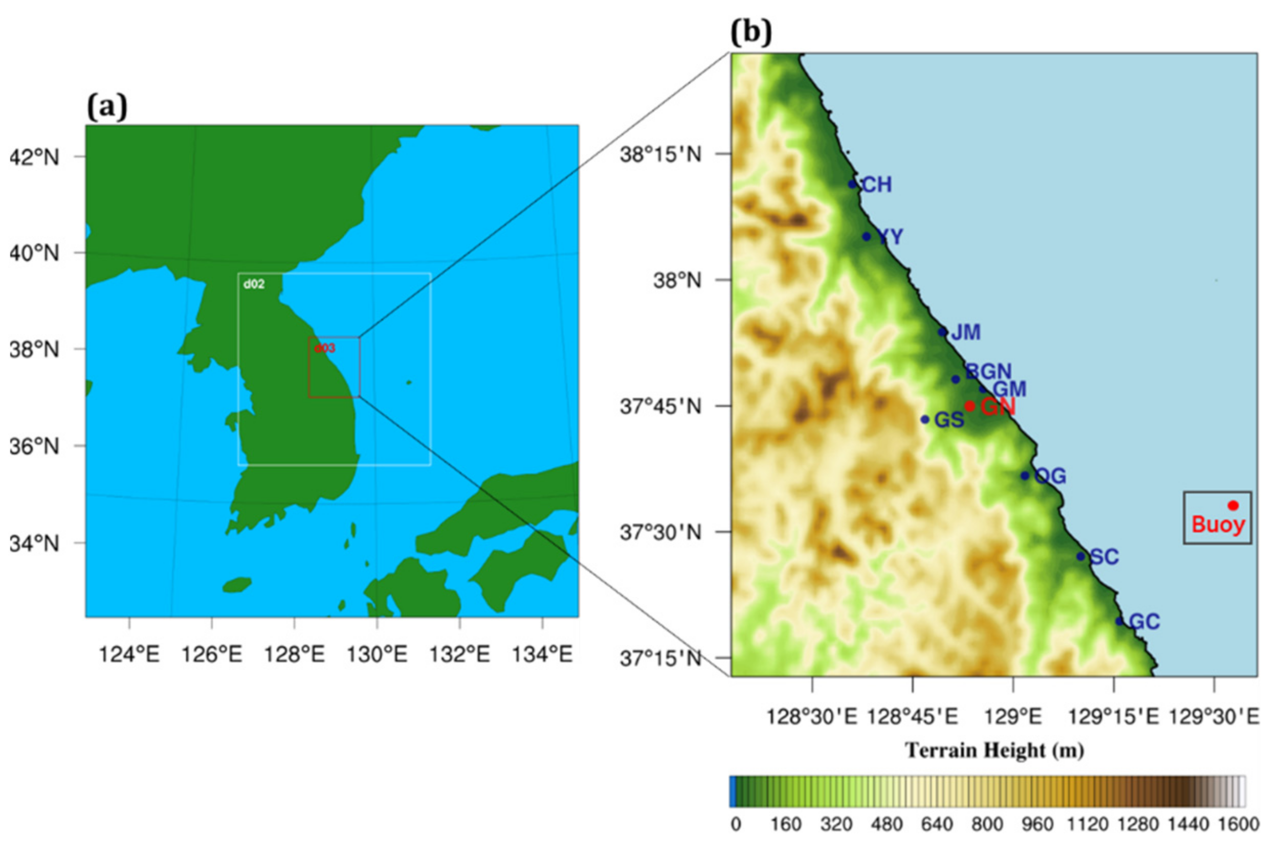
2. Data and Sea Breeze Cases

The meteorological data observed by the Korea Meteorological Administration (KMA) are provided to users after data processing in the quality control (QC) system. The Automatic Weather Station (AWS) measures temperature, pressure, humidity, wind, and precipitation every minute. The Wind Profiler Radar (WPR) is an operating device that uses electromagnetic signals to remotely sense wind speed and direction at various altitudes above the ground every 10 min. In Yeongdong region, Bukgangneung (BGN) has the only WPR operating station. We employed 1 h interval data from 8 AWS and 1 WPR of the KMA near the coast of Yeongdong for optimization and validation (see Figure 1b). Table 1 describes the main attributes of the stations. The meteorological variables used in this study are 2 m temperature, 2 m relative humidity, and 10 m wind (speed and direction) of the AWSs, and the vertical wind structure from the WPR.

We used the sea breeze selection algorithm of Hwang et al. [14] to select the sea breeze cases in the Yeongdong region. For the selection of the sea breeze cases, several meteorological variables at Gangneung (GN) and a buoy station over the sea near Okgye and Samcheok are used, including precipitation, wind direction, air temperature, and sea level pressure. Station GN is an Automated Surface Observing System (ASOS) station located about 5.2 km inland from the coast (Figure 1b). The buoy station is located approximately 70 km seaward from the coast between Okgye and Samcheok.

Based on a data set from 2009 to 2018, Hwang et al. [14] reported that GN had a total of 595 days of sea breezes, which occurred most frequently in April—June with a total of 268 days. As the initial and boundary conditions for WRF are provided by the high-resolution global final analysis (FNL) data, which have been produced since July 2015 by the National Centre for Environmental Prediction (NCEP)’s Global Forecast System (GFS), we have selected our sea breeze cases for the period of April—June from 2016 to 2021. This period depicted the lowest monthly precipitation and the largest difference in surface temperature between sea and land.

Although sea breeze is a day-by-day phenomenon routinely observed in coastal areas, it is hard to be discerned from the synoptic scale winds. Thus, we applied strict rules to select the sea breeze cases for this study, first by excluding the days with precipitation to reduce the impact of synoptic fields, and then by including the following days: (1) when the wind direction is sustained between 0° and 110° for more than 6 h during the daytime, considering the north-northwest–south-southeast orientation of the coastline in Yeongdong; (2) when the wind direction is sustained between 110° and 360° for more than 6 h during the nighttime; (3) when the land surface temperature is higher than the sea surface temperature for more than 6 consecutive h during the daytime; and (4) when the sea level pressure over the sea is 0.5 hPa higher than that over the land. Through this procedure, we have selected the following sea breeze cases for this study: 16 April 2018, 12 April 2019, and 3 May 2019 for optimization, and 17 April 2018, 11 April 2020, and 15 April 2021 for validation.

3. Methods

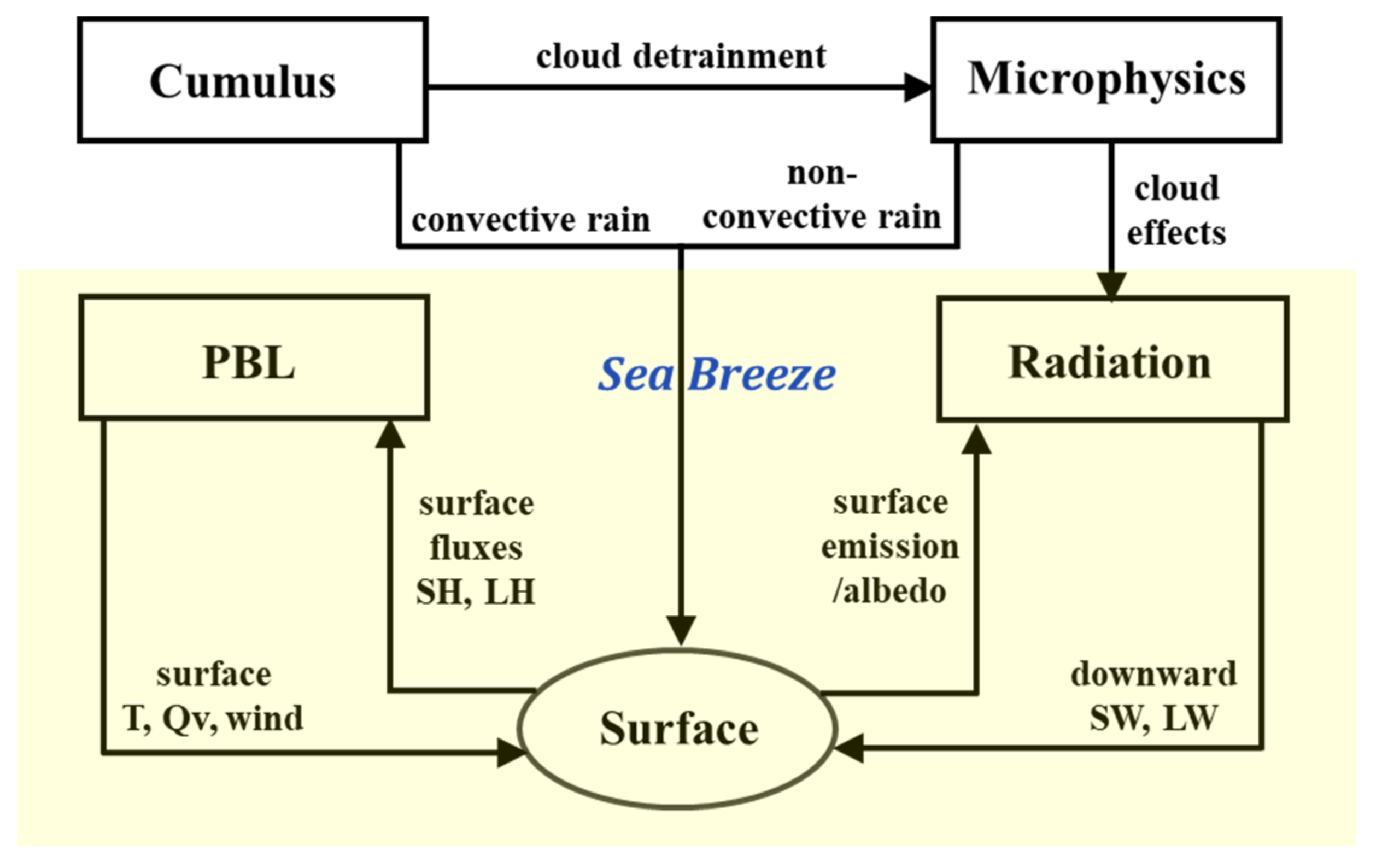
3.1. WRF Physical Parameterization Schemes

Numerical simulations of sea breezes rely on the subgrid-scale physical processes of the given model, including the PBL, land surface, radiation physics, etc. [5,15,16,17,18]. They significantly affect the sea breeze circulation through the interaction between the sea/land surface and the lower atmosphere. Figure 2 shows the schematic diagram of direct interactions among the physical processes and their parameters in WRF [30].

To search for the optimal combination of physical parameterization schemes that fits best the observed sea breeze circulations, we selected a total of 18 parameterization schemes out of four categories of physical processes in WRF: eight schemes in PBL process, four schemes in land surface physics, three schemes in shortwave radiation, and three schemes in longwave radiation (see

Table 2. Physical parameterization schemes of the WRF model used for the optimization with the option numbers the same as in the WRF namelist. The non-local closure schemes are YSU, ACM2, and TEMF scheme. The local closure schemes are MYJ, QNSE, MYNN2, BouLac, and UW scheme.

PBL Schemes			Land Surface Schemes		Radiation Schemes
Option	Scheme	Surface Layer Scheme	Option	Scheme	Option	Shortwave
1	YSU	MM5 similarity	1	TD	1	Dudhia
2	MYJ	ETA similarity	2	Noah	3	CAM
4	QNSE	QNSE	3	RUC	4	RRTMG
5	MYNN2	MYNN	4	Noah-MP	Option	Longwave
7	ACM2	MM5 similarity			1	RRTM
8	BouLac	MM5 similarity			3	CAM
9	UW	MM5 similarity			4	RRTMG
10	TEMP	TEMF

). Each PBL scheme is related to one or more surface layer schemes. We selected a frequently used surface layer scheme with each PBL based on PBL sensitivity studies [31,32,33]. The five PBL schemes (YSU, MYJ, ACM2, BouLac, and UW) use the MM5 and ETA surface-layer schemes based on the Monin–Obukhov similarity theory. The other three PBL schemes (QNSE, MYNN2, and TEMP) use their own special surface layer schemes. The shortwave and longwave radiation schemes are optimized using the pairs of same option numbers in WRF (see Table 2). The option numbers in Table 2 are the same as those in the WRF namelist.

3.1.1. Planetary Boundary Layer Scheme

For the PBL schemes, we selected three non-local and five local closure schemes. The non-local closure schemes are YonSei University (YSU) scheme [34], Asymmetrical Convective Model version 2 (ACM2) scheme [35], and Total Energy-Mass Flux (TEMF) scheme [36]. The local closure schemes are Mellor–Yamada–Janjic (MYJ) scheme [37], Quasi-Normal Scale Elimination (QNSE) scheme [38], Mellor–Yamada–Nakanishi–Niino level-2.5 (MYNN2) scheme [39], Bougeault–Lacarrere (BouLac) scheme [40], and University of Washington (UW) scheme [41].

Local schemes only consider vertical levels that are immediately adjacent in the model, whereas non-local schemes can consider deeper layers containing multiple levels when exhibiting the effect of vertical mixing through PBL.

The YSU scheme [34] is a 1.0-order non-local scheme with an explicit entrainment layer and a parabolic K-profile in an unstable mixed layer. It is a modified version of the Medium Range Forecast (MRF) scheme from the legacy MM5 model. The YSU scheme determines PBL height where the bulk Richardson number (Ri_b) exceeds a threshold value of 0 for the stable flow while it is 0.25 for the unstable flow.

The MYJ scheme [37] is a 1.5-order prognostic turbulent kinetic energy (TKE) scheme with local vertical mixing and has been used in the operational Eta model. It determines the PBL height by the level where TKE decreases to a prescribed small value of 0.2 m² s⁻².

The QNSE scheme [38] is a 1.5-order local closure scheme with a TKE prediction option to apply a new theory for stable boundary layers. It determines the PBL height as the height where the TKE profile decreases to a prescribed low value of 0.01 m² s⁻².

The MYNN2 scheme [39] is a 1.5-order local closure scheme that predicts the sub-grid TKE terms. Like the QNSE scheme, MYNN2 is a local scheme based on the comparison with large eddy simulations. The PBL height is defined as the height where the TKE falls below a critical value of 1.0 × 10⁻⁶ m² s⁻².

The ACM2 scheme [35] is a 1.0-order non-local closure scheme that describes non-local upward mixing and local downward mixing. It is a hybrid closure scheme that uses local closure for stable conditions and non-local closure for unstable conditions. The PBL height is determined as the height where the Ri_b exceeds a threshold value of 0.25.

The BouLac scheme [40] is a 1.5-order local closure scheme with a TKE prediction formulation designed for use with the BEP (Building Environment Parameterization) multi-layer urban canopy model [42]. It diagnoses the PBL height by a level where the prognostic TKE reaches a sufficiently low value of 0.005 m² s⁻².

The UW scheme [41] is a 1.5-order local TKE closure scheme. It is from the Community Earth System Model [43]. The PBL height is determined as the inversion between grid levels via a Ri_b critical value of 0.25 used in all stability cases, the same as the ACM2 scheme.

The TEMF scheme [36] is a 1.5-order non-local closure scheme, which has the subgrid-scale total energy prognostic variable and mass-flux type shallow convection. The PBL height is calculated through a Ri_b method with a threshold value of 0.

3.1.2. Land Surface Scheme

We selected four land surface schemes as candidates for optimal combination of physical parameterization schemes. They are the 5-layer thermal diffusion scheme (TD) [44], Rapid Update Cycle (RUC) [45], Noah scheme [46,47], and Noah land surface model with multiple parameterization options (Noah-MP) scheme [48].

The TD scheme [44] is the simplest in the land surface model, where only soil temperature is calculated in five soil layers with thicknesses of 1, 2, 4, 8, and 16 cm. Soil temperature is computed using the force–restore method to solve the thermal diffusion equation. Soil moisture is determined using a season-dependent function of land use. It does not include representations of the soil moisture, vegetation, and snow processes.

The RUC scheme [45] solves the heat diffusion and moisture transfer equations for nine layers from 0 to 300 cm, and it is well characterized by the soil temperature, soil moisture, and snow [49]. It comprises a thin layer covering the surface, including half of the first atmospheric layer and half of the topsoil layer, to adequately address energy budgets and embraces the part of canopy moisture and soil texture to account for vegetation impact on evaporation. This scheme represents different phases of the soil surface water, vegetation effects, and canopy water.

The Noah scheme [46,47] calculates soil temperature and soil moisture in four soil layers with thicknesses of 10, 30, 60, and 100 cm, including vegetation and snow processes. Soil temperature and moisture are computed using the soil thermal diffusion and hydrological equations, considering the surface energy and water budgets. In addition, it includes explicit physics for the vegetation and hydrological processes, i.e., evapotranspiration, canopy resistance, surface runoff, soil drainage, albedo, and urban canopy.

The Noah-MP scheme [48] followed most of the Noah scheme with the revision to the overall frame. The revised physics includes the dynamic vegetation and its ecological processes and descriptions of the snow and underground water processing. The Noah-MP scheme can use multiple options for each physical parameterization. In this study, we adopted the default options of each physical parameterization sub-scheme in the WRF model.

3.1.3. Radiation Scheme

We selected Dudhia [50], NCAR Community Atmospheric Model (CAM) [51], and Rapid Radiative Transfer Model for GCMs (RRMTG) [52] for the shortwave radiation scheme. The longwave radiation schemes include Rapid Radiative Transfer Model (RRTM) [53], NCAR Community Atmospheric Model (CAM) [51], and RRMTG [52] (Table 2).

The Dudhia shortwave radiation [50] scheme is taken from MM5. It includes a simple downward calculation of solar flux that accounts for clean-air scattering, water vapor absorption, cloud absorption, and reflection. The RRTM longwave radiation scheme [53] is a spectral-band scheme using the correlated-k method, with a specified ozone profile that interacts with resolved clouds.

The CAM shortwave and longwave radiation schemes [51] are spectral-band shortwave and longwave schemes used in the NCAR Community Atmosphere Model for climate simulations. The shortwave spectrum is divided into 19 bands, and the longwave spectrum is divided into 8 bands. This parameterization can interact with cloud fractions, aerosols, and trace gases.

The RRTMG shortwave and longwave radiation schemes [52] are widely used for weather and climate applications globally and regionally. The shortwave scheme includes 14 shortwave bands, and the longwave scheme contains 16 bands with specified ozone profile, CO₂, and trace gases.

3.2. Micro-Genetic Algorithm

The Genetic Algorithm (GA), developed by John Holland in the 1970s [25], is a global optimization algorithm based on Charles Darwin’s theory of natural selection. The fundamental mechanism of GA is to evaluate individuals in a generation to select an elite based on a fitness function (natural selection), bear new offspring using the genes in the chosen elite through a crossover mechanism, and then reconstitute a new generation with the offspring. While the reconstitutions with the natural selection and crossover mechanism are repeated, the generations evolve and converge to the optimum. The evolution with the natural selection and crossover process continues until the best solution is found or max generations are satisfied.

The GA needs many computing resources for searching for optimal solutions. The micro-GA effectively reduces computing resources using a smaller population than GA, applying reinitialization instead of the mutation process of GA [29].

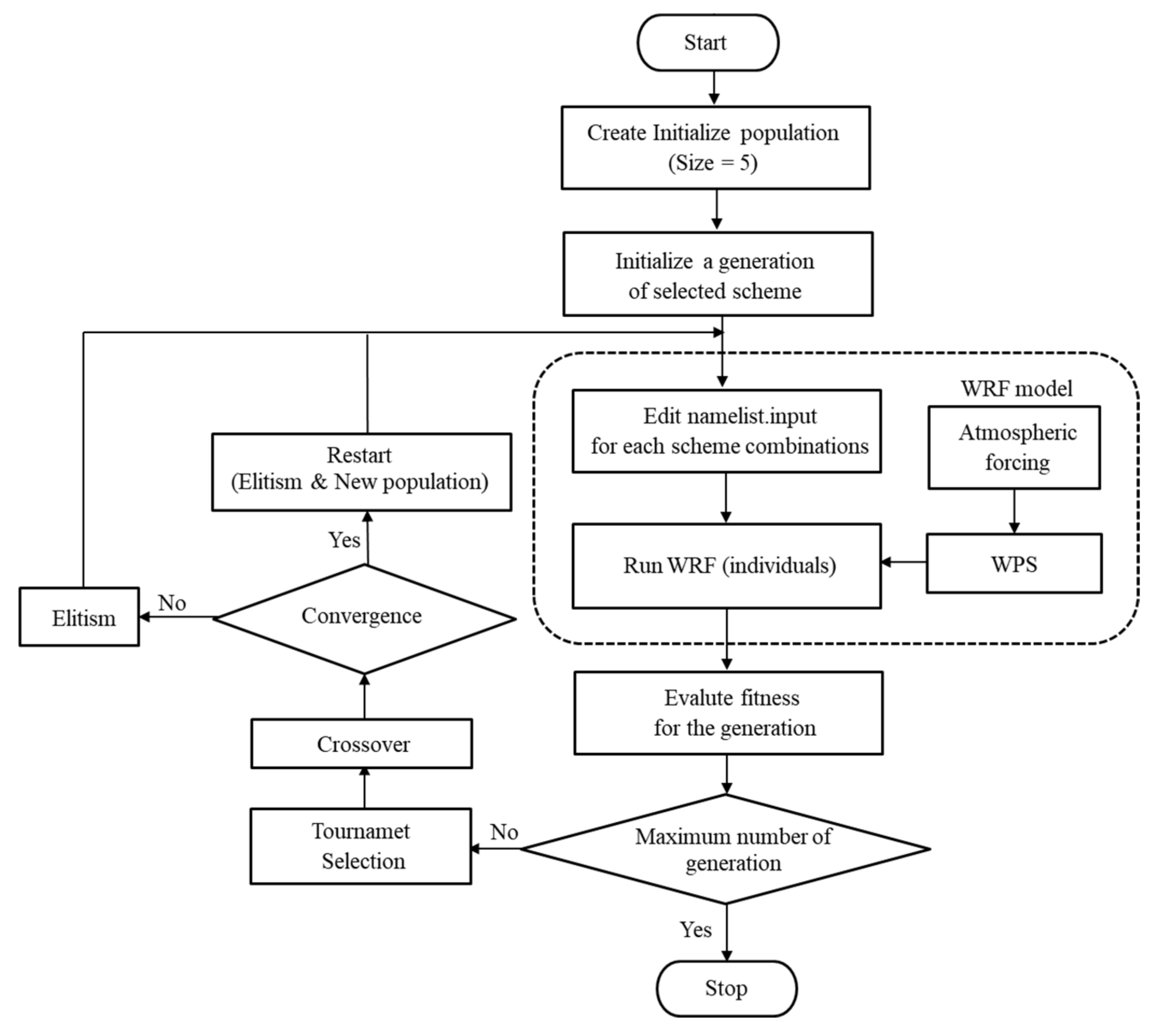
3.2.1. WRF-μGA System

In this study, we designed the model optimization system by applying the micro-GA algorithm coupled with the WRF model (WRF-μGA system) to find an optimal combination of the physical parameterization schemes for the sea breeze. The system is designed to simultaneously optimize multiple sea breeze cases, effectively performing model optimization based on the scheme for sea breeze. The WRF-μGA system is represented in the algorithm flow chart (Figure 3). A detailed description of the system is as follows: (1) The micro-GA creates a random population of the chromosomes consists of binary code when the algorithm is initialized. Here, population means the combination of physical parameterization schemes; (2) The WRF model runs with a modified namelist file by applying each scheme combination; (3) The WRF model corresponding to each individual is run and evaluated against observational data using the fitness function. Then, the selected scheme combination through tournament selection is inherited by the offspring using the crossover mechanism; (4) If the nominal convergence occurs, re-initialization is performed to generate the individuals randomly except for the elite; (5) This process continues until the maximum generation number is reached.

3.2.2. Fitness Function

In micro-GA optimization, we need to define an appropriate fitness function. Because the GA uses only one fitness function, we should be cautious about organizing a fitness function. In this study, we defined a normalized RMSE as the fitness function to obtain an appropriate assessment for variables with different scales. Since our experiments focus on sea breeze forecasting, the fitness function is based on surface meteorological variables and vertical wind profile, which are critical data for sea breeze forecasting. The fitness function is defined as follows:

$$Fitness Function=NRMS{E}_{sfc}+NRMS{E}_{ver}$$

(1)

where $NRMS{E}_{sfc}$ and $NRMS{E}_{ver}$ are defined as

$$NRMS{E}_{sfc}=NRMS{E}_{T_{2m}}+NRMS{E}_{R{H}_{2m}}+NRMS{E}_{W{S}_{10m}}+NRMS{E}_{W{D}_{10m}}$$

(2)

$$NRMS{E}_{ver}=NRMS{E}_{WS}+NRMS{E}_{WD}.$$

(3)

Here, $NRMSE$ can be calculated by normalizing $RMSE$ by the standard deviation of observations ($\sigma$) as

$$NRMSE=\frac{RMSE}{\sigma },$$

(4)

and RMSEs are given by

$$RMSE=\sqrt{\frac{1}{K\times S\times T}{\displaystyle \sum }_{k=1}^K{\displaystyle \sum }_{s=1}^S{\displaystyle \sum }_{t=1}^T{\left( F_{kst}-O_{kst} \right)}^2 }$$

(5)

for the surface variables ($T_{2m}$, $R{H}_{2m}$,$W{S}_{10m}$, and $W{D}_{10m}$) and

$$RMSE=\sqrt{\frac{1}{K\times T\times L}{\displaystyle \sum }_{k=1}^K{\displaystyle \sum }_{t=1}^T{\displaystyle \sum }_{l=1}^L{\left(F_{ktl}-O_{ktl}\right)}^2 }$$

(6)

for the vertical wind profile ($WS$ and $WD$). Here, subscripts sfc and ver indicate surface variables and wind variables at vertical levels; $K$, S, T, and L denote the number of the sea breeze cases, observational stations, observations with an interval of 1 h, and model vertical levels below 1 km, respectively (K = 3, S = 8, T = 11, L = 6); F and O indicate the prediction and observation, respectively; subscripts $T_{2m}$, $R{H}_{2m}$, $W{S}_{10m}$, and $W{D}_{10m}$ indicate 2 m temperature, 2 m relative humidity, 10 m wind speed, and 10 m wind direction, respectively; subscripts $WS$ and $WD$ mean the wind speed and direction at vertical levels, respectively. Note that the smaller fitness function indicates the higher prediction performance. To calculate RMSE for the wind direction, we applied the method by Jiménez et al. [54]. The RMSE for the wind direction is calculated using the difference $\Delta d$ between the simulated (model) and observed (obs) wind directions are given by

$$\Delta d=\left\{\begin{array}{c} d_{model}-d_{obs} if d_{model}-d_{obs} \le \left|180\right| \\ d_{model}-d_{obs}-360 if d_{model}-d_{obs }>180 \\ d_{model}-d_{obs}+360 if d_{model}-d_{obs}<-180 . \end{array}\right.$$

(7)

Therefore, the values of $\Delta d$ are in the range [−180°, 180°] and the RMSE is defined as

$$RMSE=\sqrt{\frac{{{\displaystyle \sum }}_{i=1}^n{\left(\Delta d_i\right)}^2}{n}}$$

(8)

where n is the number of pairs of simulated and observed wind directions.

4. Experimental Designs

4.1. WRF Model

In this study, we use the WRF model, version 4.1.5. The horizontal domain for this study is configured with 3 two-way nested domains (Figure 1) with resolutions of 9, 3, and 1 km and with 45 eta vertical levels. The initial and boundary conditions are derived from the 6 h Global FNL at 0.25° × 0.25° grids generated by the NCEP’s GFS, and the boundary conditions are updated every 6 h. The model is initialized at 1800 UTC (0300 LST), and the simulations are carried out for 18 h in sea breeze cases. The first 6 h is considered the model spin-up period, and the next 11 h is the searching period for the optimal combination of the physical parameterization schemes in three sea breeze cases. The dynamics and physics schemes used in the study are given in

Table 3. Overview of the WRF model configuration.

	Domain 1	Domain 2	Domain 3
Horizontal resolution	9 km × 9 km	3 km × 3 km	1 km × 1 km
Vertical layers	45 eta levels
Cumulus physics	Kain-Fritsch	Kain-Fritsch	-
Microphysics	WDM 5	WDM 5	WDM 5
Initial and Boundary conditions	NCEP FNL Global Analysis Data (0.25° × 0.25°)
Initial time	2018/04/15 1800UTC	2019/04/11 1800UTC	2019/05/02 1800UTC
Forecast time	18 h (6 h spin-up)

. The default physics schemes are the Kain–Fritsch (KF) convective parameterization scheme [55], and WRF Double Moment 5-class (WDM5) [56] microphysics scheme except for the PBL, land surface, shortwave radiation, and longwave radiation scheme. The land use and land cover distribution use the 15 s Moderate Resolution Imaging Spectroradiometer (MODIS) data with the International Geosphere-Biosphere Programme (IGBP) modified 21 categories. The simulations were simultaneously initiated on 1800 UTC 15 April 2018, 1800 UTC 11 April 2019, and 1800 UTC 2 May 2019.

4.2. Optimization

The settings of the population size and evolutionary generation in the micro-GA are important for the optimization results. Thus, the population size was set to 5 and the evolutionary generation was set to 100, following Yu et al. [21] and Zhu et al. [57]. These values are typically used in micro-GA optimization. The uniform crossover method is applied with the rate of 0.5 for conserving the variety in the genetic information.

To find the optimal combination of the physical parameterization schemes, we performed the WRF-μGA on three sea breeze cases simultaneously (16 April 2018, 12 April 2019, and 3 May 2019). To focus on the sea breeze, we optimized from 0000 UTC (0900 LST) to 1000 UTC (1900 LST), considering from the average onset time of the sea breeze to the start time of the land breeze at Gangneung (see Figure 1b).

5. Results and Discussion

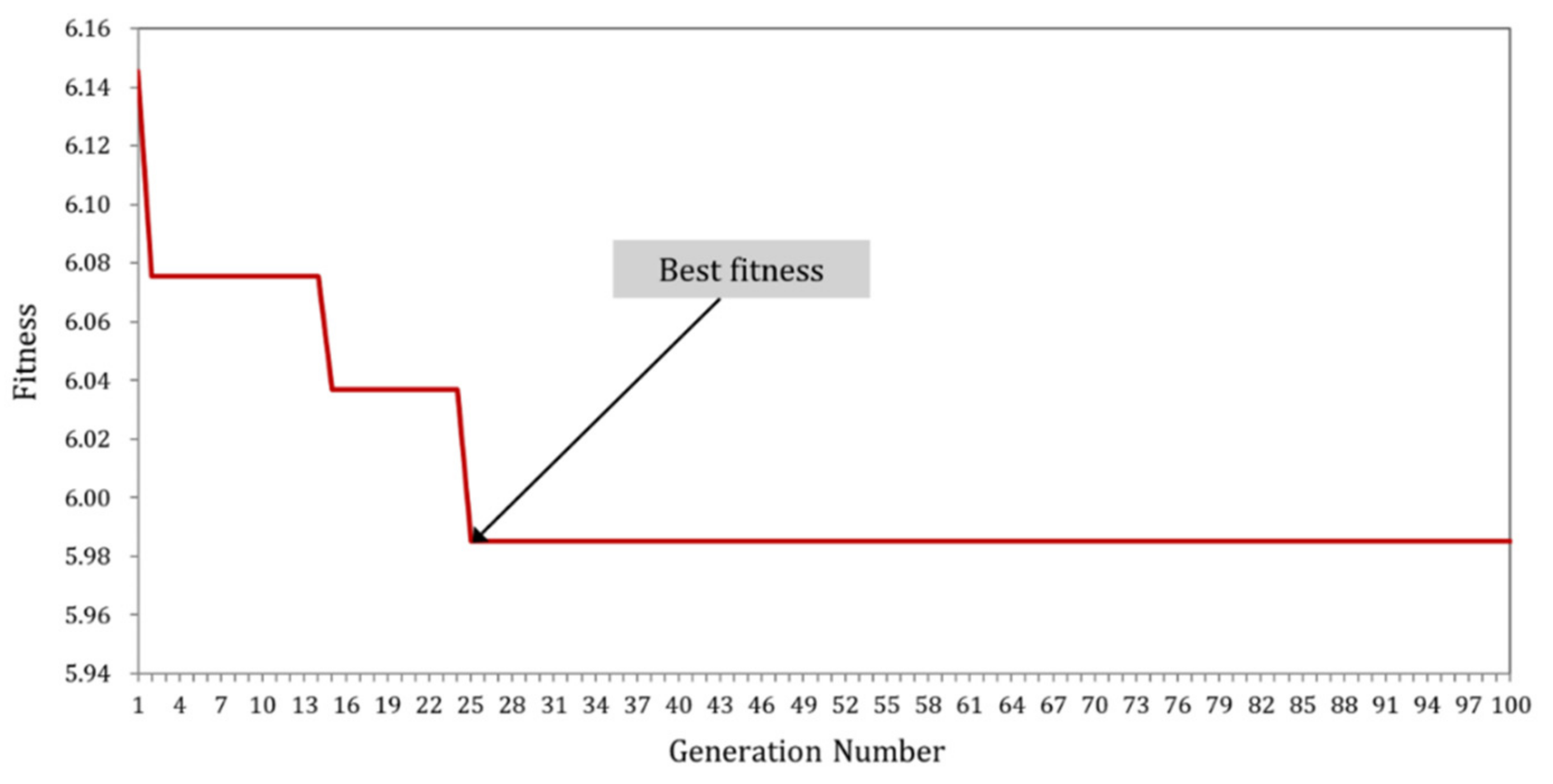
5.1. Applications of WRF-μGA System

The optimization results showed that the fitness function converged to the minimum in the 25th generation (Figure 4). The resulting optimal combination of physical parameterization schemes consisted of the MYNN2 PBL scheme, Noah-MP surface scheme, RRTMG shortwave radiation scheme, and RRTMG longwave radiation scheme. The theoretical evidence for the optimal combination of the physical parameterization schemes in coastal regions is as follows: (1) The Noah-MP scheme better represented the land-surface variables leading to more realistic simulations of the sea breeze and boundary layer characteristics at coastal regions [17,58]; (2) The MYNN2 PBL scheme has been shown to more accurately reproduce the PBL structure in coastal regions [59,60,61].

5.2. Validation

We selected three sea breeze cases for the validation: 17 April 2018, 11 April 2020, and 15 April 2021. The verification duration is 11 h at 1 h intervals from the onset time of the sea breeze to the onset time of the land breeze, which is the same as the optimization period. The surface meteorological variables, including $T_{2m}$, $R{H}_{2m}$, $W{S}_{10m}$, and $W{D}_{10m}$, and vertical wind profile variables, are compared between the model outputs and the observational data for the validation. We compared the optimal combination of the physical parameterization schemes with the combination of physical parameterization schemes mainly used in numerical simulations of the general sea breeze research [18,58,62,63].

Table 4. List of the experiments.

	Land Surface Scheme	PBL Scheme	Shortwave Radiation Scheme	Longwave Radiation Scheme	References
OPTM	Noah-MP	MYNN2	RRTMG	RRTMG	-
EXP1	Noah-MP	YSU	Dudhia	RRTM	[58]
EXP2	Noah	YSU	Dudhia	RRTM	[62]
EXP3	Noah	MYJ	Dudhia	RRTM	[18]
EXP4	TD	MYJ	Dudhia	RRTM	[63]

summarizes the combinations of the physical parameterization schemes including optimal combination scheme for the comparison experiments.

We used Equations (1)–(3) to evaluate the prediction performance in terms of all variables, surface meteorological variables, and winds at vertical levels, respectively, for different combinations of physical parameterization schemes (see Figure 5). The best performances were obtained by OPTM in terms of all variables (Figure 5a) and surface variables (Figure 5b), followed by EXP1. For the vertical wind profile variables (Figure 5c), the combination of physical parameterization schemes with the best performance differed for each sea breeze case: EXP1 on 11 April 2020 and EXP2 on 15 April 2021, respectively, outperformed OPTM. Overall, OPTM produced the best performance for the sea breeze circulations. Compared to EXP4, the largest improvement rates by OPTM, with regard to NRMSE, were as follows: 29 % for all variables on 11 April 2020 (see Figure 5a); 38 % for the surface meteorological variables on 15 April 2021 (see Figure 5b); and 24 % for the vertical wind profile variables on 11 April 2020 (see Figure 5c). Both OPTM and EXP1 showed good performances, possibly due to the influence of Noah-MP that is shown to simulate well the PBL height and heat flux associated with formation of a shallow unstable boundary layer near the coast during the sea breeze time [17].

Table 5. Statistics of surface variables (sfc) and winds at vertical levels (ver) from the experiments. Statistical indicators include bias, root mean square error (RMSE), and Pearson’s correlation coefficient (PCC).

		OPTM			EXP1			EXP2			EXP3			EXP4
		Bias	RMSE	PCC	Bias	RMSE	PCC	Bias	RMSE	PCC	Bias	RMSE	PCC	Bias	RMSE	PCC
20180417
sfc	$T_{2m}$ (°C)	−0.37	1.20	0.76	−0.97	1.48	0.78	−1.21	1.63	0.77	−0.97	1.47	0.77	−1.20	1.66	0.75
	$R{H}_{2m}\left(\%\right)$	−5.68	12.34	0.59	−3.99	13.02	0.56	−4.90	13.00	0.53	−1.53	11.37	0.58	1.44	11.99	0.58
	$W{S}_{10m}$ (m/s)	0.40	1.23	0.53	0.39	1.17	0.62	0.50	1.18	0.64	1.12	1.66	0.63	0.61	1.32	0.63
	$W{D}_{10m}$ (°)	8.58	37.85	0.44	0.56	34.27	0.56	3.55	35.62	0.54	8.39	33.19	0.55	1.15	31.48	0.57
ver	$WS$ (m/s)	−2.07	2.82	0.20	−2.17	2.92	0.12	−2.20	2.92	0.16	−1.97	2.82	0.13	−2.04	2.88	0.19
	$WD$ (°)	−1.67	80.39	0.50	−13.83	82.91	0.37	−0.31	86.78	0.49	0.38	90.07	0.32	4.5	88.64	0.14
20200411
sfc	$T_{2m}$ (°C)	−0.86	1.29	0.80	−1.10	1.55	0.79	−1.71	1.95	0.75	−1.35	1.70	0.77	−2.06	2.36	0.74
	$R{H}_{2m}\left(\%\right)$	−2.50	11.69	0.36	−1.46	12.71	0.34	−0.09	11.24	0.34	1.30	12.83	0.25	7.81	15.82	0.22
	$W{S}_{10m}$ (m/s)	0.52	1.58	0.25	0.39	1.54	0.22	0.49	1.62	0.23	1.30	2.04	0.27	0.63	1.99	0.16
	$W{D}_{10m}$ (°)	8.24	55.74	0.35	8.74	58.61	0.33	15.15	66.61	0.26	11.23	64.62	0.29	13.93	83.79	0.23
ver	$WS$ (m/s)	−0.51	1.73	0.45	−0.49	1.62	0.56	−0.99	1.98	0.35	−0.10	1.87	0.45	−1.28	2.37	−0.01
	$WD$ (°)	16.64	76.16	0.50	6.28	64.30	0.48	12.05	66.54	0.61	18.39	75.21	0.41	42.18	96.63	0.33
20210415
sfc	$T_{2m}$ (°C)	−0.55	1.10	0.76	−0.85	1.31	0.74	−1.31	1.63	0.72	−1.06	1.43	0.73	−1.62	1.98	0.62
	$R{H}_{2m}\left(\%\right)$	5.91	12.36	0.46	6.96	13.51	0.35	8.07	13.64	0.35	10.71	15.98	0.37	19.89	25.14	0.19
	$W{S}_{10m}$ (m/s)	0.87	2.03	0.39	0.78	1.93	0.41	0.91	1.86	0.48	2.21	2.83	0.57	1.12	2.038	0.49
	$W{D}_{10m}$ (°)	1.04	20.83	0.72	0.03	23.73	0.70	3.03	22.94	0.69	4.85	24.29	0.67	13.41	36.21	0.48
ver	$WS$ (m/s)	−1.52	3.32	−0.25	−1.35	3.11	−0.20	−1.11	2.92	−0.17	−1.14	3.35	−0.23	−1.44	3.15	−0.19
	$WD$ (°)	1.60	61.71	0.47	15.00	67.26	0.43	16.35	63.65	0.40	7.14	64.16	0.44	22.80	71.53	0.25

summarizes the statistical results of the model performances in surface meteorological variables and wind variables at vertical levels. The results of RMSE and Bias are as follows: the OPTM showed the best results in all sea breeze cases for $T_{2m}$ and indicated good performance of $W{D}_{10m}$ and $WD$. In $T_{2m}$, all experiments showed underestimation with a cold bias, and OPTM showed the best performance. In $R{H}_{2m}$, OPTM, EXP2, and EXP3 performed well in each case. In $W{S}_{10m}$, EXP1 simulated the closest to observation while the performance of OPTM is moderate. $W{S}_{10m}$ was overestimated, which was consistent with various studies using WRF [33,61].

The overestimation is partly caused by the uncertainty in the sub-grid surface roughness and its associated turbulence at low atmospheric levels [54]. In $W{D}_{10m}$, OPTM showed good performance. In $WS$ and $WD$, OPTM and EXP1 showed good performance, and OPTM performance was better in $WD$. The Pearson’s correlation coefficient (PCC) was used to identify the correlation between simulation and observation for each meteorological variable. Generally, a value of PCC greater than 0.7 is considered a strong correlation, and anything less than 0.4 is considered a weak or no correlation. In most experiments of the three cases, $T_{2m}$ showed a strong correlation greater than 0.7. However, all experiments showed weak correlations less than 0.4 in $R{H}_{2m}$, $W{S}_{10m}$, and $W{D}_{10m}$ on 11 April 2020. The $WS$ showed a weak negative correlation in all experiments on 15 April 2021. Overall, OPTM indicated good performance results in most sea breeze cases for $T_{2m}$, $R{H}_{2m}$, $W{D}_{10m}$, and $WD.$

Figure 6 shows the time series of surface meteorological variables averaged for 8 observation stations on 17 April 2018, 11 April 2020, and 15 April 2021. In $T_{2m}$ (Figure 6a), OPTM simulated the closest to the observations for the sea breeze circulation. In $R{H}_{2m}$ (Figure 6b), EXP3 and EXP4 were closer to observation, and all experiments showed dry bias until 0600 UTC (15 LST) when the sea breeze was the strongest: OPTM was the closest to observation after 0600 UTC, and most experiments showed dry bias on 17 April 2018. Diurnal variations in $R{H}_{2m}$ were well represented and was inversely related to $T_{2m}$, as expected. The EXP2 appeared close to observation and showed dry bias until 0500 UTC (14 LST) when the sea breeze was the strongest, whereas OPTM was the closest to observation after 0500 UTC on 11 April 2020. All the experiments except for EXP4 showed similar trends, and OPTM was closest to the observation on 15 April 2021.

However, moist bias became large after 0400 UTC (13 LST) when the sea breeze was strong. In $W{S}_{10m}$ (Figure 6c), OPTM and EXP1 were closest to observation: compared to other meteorological variables, the pattern of overestimation was more significant, especially on 15 April 2021, which is common in the wind speed prediction using WRF [61,64]. In $W{D}_{10m}$ (Figure 6d), at the onset time of the sea breeze, the observations showed a change in the wind direction, from south-southwest to east at 0000 UTC (0900 LST) on 17 April 2018, from southwest to southeast at 0800 LST on 11 April 2020, and from southwest to southeast at 0000 UTC on 15 April 2021. The OPTM simulated well the onset time of the sea breeze on 17 April 2018 and 15 April 2021; however, on 11 April 2020, the sea breeze onset time was delayed by 1 h in OPTM and by 2 h in the other experiments. Therefore, OPTM captured well the timing of changing from sea breeze to land breeze in all the three cases.

5.3. Sensitivity Analysis

The development and growth of PBL depends on the surface heat and moisture fluxes and their upward mixing by the turbulent eddies and subsidence [64,65]. The advection of cold and moist air by sea breeze can lead to important modifications to the land surface fluxes, and thus have consequences on the boundary layer development. [66]. In other words, the sea breezes move cold and moist air inland, lowering the air temperature, weakening the convection structure, and eventually impeding the growth of PBL. Therefore, in this study, sensitivity analysis was performed on the wind vertical structure of the sea breeze and PBL height at Gangneung, a representative area of Yeongdong for the optimized set of the schemes and the various other sets.

Figure 7 shows the time variation of the vertical wind profile and PBL height for the experiments of OPTM and EXP1—EXP4 on 15 April 2021. In OPTM, the PBL height started to grow due to solar radiation in the morning and reached the peak at 1100 LST (Figure 7a). After that, the PBL height began to decrease as the sea breeze became stronger. In particular, the PBL height appeared lowest at 0500–0600 UTC (1400–1500 LST), which grew slightly again: this feature is strongly linked to the sea breeze circulation whose intensity was the strongest at 0500–0600 UTC, and then decreased slightly. Both OPTM and EXP1 use Noah MP and show similar features in the PBL height and horizontal wind vector: this is reasonable because LSM calculates the heat and moisture fluxes for land and provides the lower boundary conditions for vertical transport in the PBL. However, in EXP1, the peak PBL height appeared at 0300 UTC (1200 LST), 1 h later than that in OPTM (Figure 7b); this is strongly related to the delay in the sea breeze development—mainly caused by different choices of the physical parameterization schemes other than LSM (see Table 4). In EXP2, the peak of PBL height also appeared at 0300 UTC, similarly to EXP1 (Figure 7c): the only difference between EXP1 and EXP2 is in LSM where the latter employed Noah LSM. Both EXP2 and EXP3 share the same parameterization schemes except for the PBL scheme—YSU for EXP2 and MYJ for EXP3 (see Table 4)—which resulted in unreasonable PBL features in EXP3 (Figure 7d). EXP4 is different from EXP3 only in LSM, i.e., 5-Layer scheme in EXP4 vs. Noah LSM in EXP3, but it showed much unreasonable PBL evolution compared to EXP3 (Figure 7e). Overall, the PBL structure and evolution got adjusted to show better features with the optimized set of parametrization schemes.

6. Conclusions

This study aimed to improve the forecast skill of the sea breeze circulation along the east coast of Yeongdong in the Korean Peninsula by finding the optimal set of physical parameterization schemes in the Weather Research and Forecasting (WRF) using a global optimization method called the micro-Genetic Algorithm (GA). We developed a system that combines the WRF and the micro-GA (WRF-μGA) and applied it to a combinational optimization problem.

We selected nine observation stations in Yeongdong coastal region of the Korean Peninsula for the optimization and validation. The fitness function was composed of the normalized root mean squared error (RMSE) considering $T_{2m}$, $R{H}_{2m}$, $W{S}_{10m}$, $W{D}_{10m}$, $WS$, and $WD$. We simultaneously optimized three sea breeze cases selected by the sea breeze selection algorithm. Based on the WRF-μGA system, we found that the optimal combination consists of the MYNN2 (PBL), Noah-MP (land surface), RRTMG (shortwave radiation), and RRTMG (longwave radiation) schemes.

We first conducted validation tests for the variables used for optimization and confirmed that the optimized model results showed generally good matches with the observations. We then compared the optimized vs. non-optimized experiments and found that the overall performance of WRF using the optimal parameterization scheme set (OPTM) was excellent in sea breeze simulations. We noticed that an experiment with the scheme set of YSU, NoahMP, Dudhia, and RRTM also showed comparable performance. The YSU and MYNN2 schemes simulated well the PBL structure in the coastal areas and the sea breezes, respectively, in previous studies: the Noah-MP, commonly employed in the two experiments is also known as the best land surface scheme for simulating the sea breeze circulation. In the sensitivity experiments, we found that the optimized set of parameterization schemes was adjusted to show better features of the PBL structure and evolution.

We conclude that the dynamical and thermodynamical characteristics of sea breeze circulation can be analyzed more accurately using the optimal combination of the physical parameterization schemes, obtained by the WRF-μGA system; thus, this kind of combinational optimization can lay the foundation for understanding the local circulations and meteorological phenomena in the coastal areas, including the low-level air convergence, precipitation, and atmospheric pollutant.

References

1. Simpson, J.E. Sea Breeze and Local Winds; Cambridge University Press: Cambridge, UK, 1994; 234p. [Google Scholar]
2. Miller, S.T.K.; Keim, B.D.; Talbot, R.W.; Mao, H. Sea breeze: Structure, forecasting, and impacts. Rev. Geophys. 2003, 41, 31. [Google Scholar] [CrossRef] [Green Version]
3. Bhate, J.; Kesarkar, A.P.; Karipot, A.; Subrahamanyam, D.B.; Rajasekhar, M.; Sathiyamoorthy, V.; Kishtawal, C.M. A sea breeze induced thunderstorm over an inland station over Indian South Peninsula—A case study. J. Atmos. Sol. Terr. Phys. 2016, 148, 96–111. [Google Scholar] [CrossRef]
4. Lee, D.-I.; Han, Y.-H. Vertical distribution of aerosol concentrations in the boundary layer observed by a tethered balloon: Part II: Distributions of aerosol concentrations in relation to the sea breeze front. J. Korean Meteor. Soc. 1992, 28, 497–507. [Google Scholar]
5. Salvador, N.; Loriato, A.G.; Santiago, A.; Albuquerque, T.T.A.; Reis, N.C., Jr.; Santos, J.M.; Landulfo, E.; Moreira, G.; Lopes, F.; Held, G. Study of the thermal internal boundary layer in sea breeze conditions using different parameterizations: Application of the WRF model in the Greater Vitória region. Rev. Bras. Meteorol. 2016, 31, 593–609. [Google Scholar] [CrossRef] [Green Version]
6. Nam, H.G.; Kim, B.G.; Han, S.O.; Lee, C.K.; Lee, S.S. Characteristics of easterly-induced snowfall in Yeongdong and its relationship to air-sea temperature difference. Asia Pac. J. Atmos. Sci. 2014, 50, 541–552. [Google Scholar] [CrossRef]
7. Park, M.-S.; Chae, J.-H. Features of sea–land-breeze circulation over the Seoul metropolitan area. Geosci. Lett. 2018, 5, 28. [Google Scholar] [CrossRef] [Green Version]
8. Lim, H.-J.; Lee, Y.-H. Characteristics of sea breezes at coastal area in Boseong. Atmosphere 2019, 29, 41–51, (In Korean with English abstract). [Google Scholar]
9. Park, S.K.; Park, S. On a flood-producing coastal mesoscale convective storm associated with the Kor’easterlies: Multi-data analyses using remote sensing, in-situ observations and storm-scale model simulations. Remote Sens. 2020, 12, 1532. [Google Scholar] [CrossRef]
10. Lee, J.G.; Lee, J.S. A numerical study of Yeongdong heavy snowfall events associated with easterly. J. Korean Meteor. Soc. 2003, 39, 475–490, (In Korean with English abstract). [Google Scholar]
11. Park, S.K.; Lee, E. Synoptic features of orographically enhanced heavy rainfall on the east coast of Korea associated with Typhoon Rusa (2002). Geophys. Res. Lett. 2007, 34, L02803. [Google Scholar] [CrossRef] [Green Version]
12. Lee, J.G.; Kim, Y.J. A numerical simulation study using WRF of a heavy snowfall event in the Yeongdong coastal area in relation to the northeasterly. Atmosphere 2008, 18, 339–354, (In Korean with English abstract). [Google Scholar]
13. Tsai, C.-L.; Kim, K.; Liou, Y.-C.; Lee, G.; Yu, C.-K. Impacts of topography on airflow and precipitation in the Pyeongchang area seen from multiple-Doppler radar observations. Mon. Wea. Rev. 2018, 146, 3401–3424. [Google Scholar] [CrossRef]
14. Hwang, H.W.; Eun, S.H.; Kim, B.G.; Park, S.J.; Park, G.M. Occurrence characteristics of sea breeze in the Gangneung region for 2009~2018. Atmosphere 2020, 30, 221–236, (In Korean with English abstract). [Google Scholar]
15. Srinivas, C.V.; Venkatesan, R.; Singh, A.B. Sensitivity of mesoscale simulations of land–sea breeze to boundary layer turbulence parameterization. Atmos. Environ. 2007, 41, 2534–2548. [Google Scholar] [CrossRef]
16. Steele, C.J.; Dorling, S.R.; von Glasow, R.; Bacon, J. Idealized WRF model sensitivity simulations of sea breeze types and their effects on offshore windfields. Atmos. Chem. Phys. 2013, 13, 443–461. [Google Scholar] [CrossRef] [Green Version]
17. Reddy, B.R.; Srinivas, C.V.; Shekhar, S.S.; Baskaran, R.; Venkatraman, B. Impact of land surface physics in WRF on the simulation of sea breeze circulation over southeast coast of India. Meteorol. Atmos. Phys. 2020, 132, 925–943. [Google Scholar] [CrossRef]
18. Salvador, N.; Reis, N.C., Jr.; Santos, J.M.; Albuquerque, T.T.A.; Loriato, A.G.; Delbarre, H.; Augustin, P.; Sokolov, A.; Moreira, D.M. Evaluation of Weather Research and Forecasting model parameterizations under sea-breeze conditions in a North Sea coastal environment. J. Meteorol. Res. 2016, 30, 998–1018. [Google Scholar] [CrossRef]
19. Hock, N.; Pu, Z. Numerical simulations of the Florida sea breeze and its associated convection with the WRF model. In Proceedings of the 28th Conference on Weather Analysis and Forecasting/24th Conference on Numerical Weather Prediction, Seattle, WA, USA, 25 January 2017; American Meteorological Society: Boston, MA, USA, 2017; p. 1181. [Google Scholar]
20. Lee, Y.H.; Park, S.K.; Chang, D.-E. Parameter estimation using the genetic algorithm and its impact on quantitative precipitation forecast. Ann. Geophys. 2006, 24, 3185–3189. [Google Scholar] [CrossRef]
21. Yu, X.; Park, S.K.; Lee, Y.H.; Choi, Y.-S. Quantitative precipitation forecast of a tropical cyclone through optimal parameter estimation in a convective parameterization. SOLA 2013, 9, 36–39. [Google Scholar] [CrossRef] [Green Version]
22. Hong, S.; Yu, X.; Park, S.K.; Choi, Y.-S.; Myoung, B. Assessing optimal set of implemented physical parameterization schemes in a multi-physics land surface model using genetic algorithm. Geosci. Model. Dev. 2014, 7, 2517–2529. [Google Scholar] [CrossRef] [Green Version]
23. Hong, S.; Park, S.K.; Yu, X. Scheme-based optimization of land surface model using a micro-genetic algorithm: Assessment of its performance and usability for regional applications. SOLA 2015, 11, 129–133. [Google Scholar] [CrossRef] [Green Version]
24. Park, S.; Park, S.K. A micro-genetic algorithm (GA v1.7.1 a) for combinatorial optimization of physics parameterizations in the Weather Research and Forecasting model (v4.0.3) for quantitative precipitation forecast in Korea. Geosci. Model. Dev. 2021, 14, 6241–6255. [Google Scholar] [CrossRef]
25. Holland, J.H. Adaptation in Natural and Artificial System: An Introductory Analysis with Applications to Biology, Control, and Artificial Intelligence; University of Michigan Press: Ann Arbor, MI, USA, 1975; 183p. [Google Scholar]
26. Goldberg, D.E. Genetic Algorithms in Search, Optimization and Machine Learning, 13th ed.; Addison-Wesely Publishing Company: Reading, MA, USA, 1989; 412p. [Google Scholar]
27. Hu, Y.M.; Ding, Y.H.; Shen, T.L. Validation of a receptor/dispersion model coupled with a genetic algorithm using synthetic data. J. Appl. Meteorol. Climatol. 2006, 45, 476–490. [Google Scholar]
28. Bastani, M.; Kholghi, M.; Rakhshandehroo, G.R. Inverse modeling of variable-density groundwater flow in a semi-arid area in Iran using a genetic algorithm. Hydrogeol. J. 2010, 18, 1191–1203. [Google Scholar] [CrossRef]
29. Krishnakumar, K. Micro-genetic algorithms for stationary and non-stationary function optimization. In Intelligent Control and Adaptive Systems, Proceedings of SPIE 1196, 1989 Symposium on Visual Communications, Image Processing, and Intelligent Robotics Systems, Philadelphia, PA, USA, 1–3 November 1989; International Society for Optical Engineering: Bellingham, WA, USA, 1990; pp. 289–296. [Google Scholar]
30. Dudhia, J. A history of mesoscale model development. Asia-Pac. J. Atmos. Sci. 2014, 50, 121–131. [Google Scholar] [CrossRef]
31. Banks, R.F.; Tiana-Alsina, J.; Rocadenbosch, F.; Baldasano, J.M. Performance evaluation of the boundary-layer height from lidar and the Weather Research and Forecasting model at an urban coastal site in the north-east Iberian Peninsula. Bound. Layer Meteorol. 2015, 157, 265–292. [Google Scholar] [CrossRef] [Green Version]
32. Banks, R.F.; Tiana-Alsina, J.; Baldasano, J.M.; Rocadenbosch, F.; Papayannis, A.; Solomos, S.; Tzanis, C.G. Sensitivity of boundary-layer variables to PBL schemes in the WRF model based on surface meteorological observations, lidar, and radiosondes during the HygrA-CD campaign. Atmos. Res. 2016, 176, 185–201. [Google Scholar] [CrossRef]
33. Avolio, E.; Federico, S.; Miglietta, M.M.; Feudo, T.L.; Calidonna, C.R.; Sempreviva, A.M. Sensitivity analysis of WRF model PBL schemes in simulating boundary-layer variables in southern Italy: An experimental campaign. Atmos. Res. 2017, 192, 58–71. [Google Scholar] [CrossRef]
34. Hong, S.Y.; Noh, Y.; Dudhia, J. A new vertical diffusion package with an explicit treatment of entrainment processes. Mon. Wea. Rev. 2006, 134, 2318–2341. [Google Scholar] [CrossRef] [Green Version]
35. Pleim, J.E. A combined local and nonlocal closure model for the atmospheric boundary layer. Part I: Model description and testing. J. Appl. Meteorol. Climatol. 2007, 46, 1383–1395. [Google Scholar]
36. Angevine, H.J.; Mauritsen, T. Performance of an eddy diffusivity-mass flux scheme for shallow cumulus boundary layers. Mon. Wea. Rev. 2010, 138, 2895–2912. [Google Scholar] [CrossRef] [Green Version]
37. Janjić, Z.I. Nonsingular Implementation of the Mellor-Yamada Level 2.5 Scheme in the NCEP Meso Model. NCEP Office Note 437; National Centers for Environmental Prediction: College Park, MD, USA, 2002; 61p. [Google Scholar]
38. Sukoriansky, S.; Galperin, B.; Perov, V. Application of a new spectral theory of stably stratified turbulence to the atmospheric boundary layer over sea ice. Bound. Layer Meteorol. 2005, 117, 231–257. [Google Scholar] [CrossRef]
39. Nakanishi, M.; Niino, H. An improved Mellor–Yamada level-3 model: Its numerical stability and application to a regional prediction of advection fog. Bound. Layer Meteorol. 2006, 119, 397–407. [Google Scholar] [CrossRef]
40. Bougeault, P.; Lacarrere, P. Parameterization of orography-induced turbulence in a mesobeta–scale model. Mon. Wea. Rev. 1989, 117, 1872–1890. [Google Scholar] [CrossRef]
41. Bretherton, C.S.; Park, S. A new moist turbulence parameterization in the Community Atmosphere Model. J. Clim. 2009, 22, 3422–3448. [Google Scholar] [CrossRef]
42. Martilli, A.; Clappier, A.; Rotach, M.W. An urban surface exchange parameterisation for mesoscale models. Bound. Layer Meteorol. 2002, 104, 261–304. [Google Scholar] [CrossRef]
43. Hurrell, J.W.; Holland, M.M.; Gent, P.R.; Ghan, S.; Kay, J.E.; Kushner, P.J.; Marshall, S. The Community Earth System Model: A framework for collaborative research. Bull. Am. Meteorol. Soc. 2013, 94, 1339–1360. [Google Scholar] [CrossRef]
44. Dudhia, J. A multi-layer soil temperature model for MM5. In Proceedings of the Sixth PSU/NCAR Mesoscale Model Users’ Workshop, Boulder, CO, USA, 22–24 July 1996; pp. 22–24. [Google Scholar]
45. Benjamin, S.G.; Grell, G.A.; Brown, J.M.; Smirnova, T.G.; Bleck, R. Mesoscale weather prediction with the RUC hybrid isentropic-terrain-following coordinate model. Mon. Wea. Rev. 2004, 132, 473–494. [Google Scholar] [CrossRef]
46. Chen, F.; Dudhia, J. Coupling an advanced land surface–hydrology model with the Penn State–NCAR MM5 modeling system. Part I: Model implementation and sensitivity. Mon. Wea. Rev. 2001, 129, 569–585. [Google Scholar] [CrossRef] [Green Version]
47. Ek, M.B.; Mitchell, K.E.; Lin, Y.; Rogers, E.; Grunmann, P.; Koren, V.; Gayno, G.; Tarpley, J.D. Implementation of Noah land surface model advances in the National Centers for Environmental Prediction operational mesoscale Eta model. J. Geophys. Res. Atmos. 2003, 108, 8851. [Google Scholar] [CrossRef]
48. Niu, G.Y.; Yang, Z.L.; Mitchell, K.E.; Chen, F.; Ek, M.B.; Barlage, M.; Xia, Y. The community Noah land surface model with multi-parameterization options (Noah-MP): 1. Model description and evaluation with local-scale measurements. J. Geophys. Res. Atmos. 2011, 116, D12109. [Google Scholar] [CrossRef] [Green Version]
49. Smirnova, T.G.; Brown, J.M.; Benjamin, S.G.; Kenyon, J.S. Modifications to the Rapid Update Cycle Land Surface Model (RUC LSM) available in the Weather Research and Forecast (WRF) model. Mon. Wea. Rev. 2016, 144, 1851–1865. [Google Scholar] [CrossRef]
50. Dudhia, J. Numerical study of convection observed during the winter monsoon experiment using a mesoscale two-dimensional model. J. Atmos. Sci. 1989, 46, 3077–3107. [Google Scholar] [CrossRef]
51. Collins, W.D.; Rasch, P.J.; Boville, B.A.; Hack, J.J.; McCaa, J.R.; Williamson, D.L.; Kiehl, J.T.; Briegleb, B. Description of the NCAR Community Atmosphere Model (CAM 3.0); NCAR Technical Note, NCAR/TN-464+STR; Technical Report; NCAR: Boulder, CO, USA, 2004. [Google Scholar]
52. Iacono, M.J.; Delamere, J.S.; Mlawer, E.J.; Shephard, M.W.; Clough, S.A.; Collins, W.D. Radiative forcing by long-lived greenhouse gases: Calculations with the AER radiative transfer models. J. Geophys. Res. Atmos. 2008, 113, D13103. [Google Scholar] [CrossRef]
53. Mlawer, E.J.; Taubman, S.J.; Brown, P.D.; Iacono, M.J.; Clough, S.A. Radiative transfer for inhomogeneous atmospheres: RRTM, a validated correlated-k model for the long-wave. J. Geophys. Res. Atmos. 1997, 102, 16663–16682. [Google Scholar] [CrossRef] [Green Version]
54. Jiménez, P.A.; Dudhia, J. Improving the representation of resolved and unresolved topographic effects on surface wind in the WRF model. J. Appl. Meteorol. Climatol. 2012, 51, 300–316. [Google Scholar] [CrossRef] [Green Version]
55. Kain, J.S. The Kain–Fritsch convective parameterization: An update. J. Appl. Meteorol. Climatol. 2004, 43, 170–181. [Google Scholar] [CrossRef] [Green Version]
56. Lim, K.-S.S.; Hong, S.-Y. Development of an effective double-moment cloud microphysics scheme with prognostic Cloud Condensation Nuclei (CCN) for weather and climate models. Mon. Wea. Rev. 2010, 138, 1587–1612. [Google Scholar] [CrossRef] [Green Version]
57. Zhu, J.; Shu, J.; Yu, X. Improvement of typhoon rainfall prediction based on optimization of the Kain-Fritsch convection parameterization scheme using a micro-genetic algorithm. Front. Earth Sci. 2019, 13, 721–732. [Google Scholar] [CrossRef]
58. Rajeswari, J.R.; Srinivas, C.V.; Rao, T.N.; Venkatraman, B. Impact of land surface physics on the simulation of boundary layer characteristics at a tropical coastal station. Atmos. Res. 2020, 238, 104888. [Google Scholar] [CrossRef]
59. Lombardo, K.; Colle, B.A. Processes controlling the structure and longevity of two quasi-linear convective systems crossing the southern New England coast. Mon. Wea. Rev. 2013, 141, 3710–3734. [Google Scholar] [CrossRef] [Green Version]
60. Tyagi, B.; Magliulo, V.; Finardi, S.; Gasbarra, D.; Carlucci, P.; Toscano, P.; Gioli, B. Performance analysis of planetary boundary layer parameterization schemes in WRF modeling set up over southern Italy. Atmosphere 2018, 9, 272. [Google Scholar] [CrossRef] [Green Version]
61. Hariprasad, K.B.R.R.; Srinivas, C.V.; Singh, A.B.; Rao, S.V.B.; Baskaran, R.; Venkatraman, B. Numerical simulation and intercomparison of boundary layer structure with different PBL schemes in WRF using experimental observations at a tropical site. Atmos. Res. 2014, 145, 27–44. [Google Scholar] [CrossRef]
62. Dewi, D.P.R.; Fatmasari, D.; Gustari, I. Simulation of sea breeze events in gulf of Jakarta under different synoptic condition: An application of WRF model. In IOP Conf. Ser.: Earth Environ. Sci., Proceedings of the International Conference on Tropical Meteorology and Atmospheric Sciences, Bandung, Indonesia, 19–20 September 2018; IOP publishing: Bristol, UK, 2019; Volume 303, p. 012045. [Google Scholar] [CrossRef] [Green Version]
63. Papanastasiou, D.K.; Melas, D.; Lissaridis, I. Study of wind field under sea breeze conditions; an application of WRF model. Atmos. Res. 2010, 98, 102–117. [Google Scholar] [CrossRef]
64. Yerramilli, A.; Challa, V.S.; Dodla, V.B.R.; Dasari, H.P.; Young, J.H.; Patrick, C.; Swanier, S.J. Simulation of surface ozone pollution in the central gulf coast region using WRF/Chem Model: Sensitivity to PBL and Land Surface Physics. Adv. Meteorol. 2010, 2010, 319138. [Google Scholar] [CrossRef] [Green Version]
65. Jain, S. WRF model analysis of land-surface processes over Jaipur Region. Int. J. Sci. Eng. Technol. 2015, 6, 1276–1284. [Google Scholar]
66. Miao, J.-F.; Wyser, K.; Chen, D.; Ritchie, H. Impacts of boundary layer turbulence and land surface process parameterizations on simulated sea breeze characteristics. Ann. Geophys. 2009, 27, 2303–2320. [Google Scholar] [CrossRef]
Figure 1. (a) Computational domain in WRF having triple nesting with horizontal resolution of 9 km (d01), 3 km (d02), and 1 km (d03) and (b) locations of the observational stations in d03. Station GangNeung (GN; in red) is used only for selecting the sea breeze cases. Since the buoy location (37.54° N, 130.0° S) is out of the range of domain 3 (d03), the buoy site (in red) is marked with a box. The wind profiler radar is located at BukGangNeung (BGN). See Table 1 for the detailed information on the stations in blue.
Applsci 11 11221 g001
Figure 2. Schematic diagram representing direct interactions among the parameterized physical process. Acronyms SW and LW represent the shortwave and longwave radiation, respectively; SH and LH indicate the sensible heat and latent heat flux, respectively. Variables T and Qv mean temperature and water vapor mixing ratio, respectively. Reproduced with permission from Dudhia, A history of mesoscale model development [30]; published by the Korean Meteorological Society and Springer, 2014.
Applsci 11 11221 g002
Figure 3. The flow chart describing the combinational optimization process from the WRF-μGA system.
Applsci 11 11221 g003
Figure 4. Evolution of the fitness function in terms of the generations during the optimization process.
Applsci 11 11221 g004
Figure 5. Comparison of the optimized vs. non-optimized experiments using the normalized RMSE for (a) all variables based on Equation (1), (b) surface variables based on Equation (2), and (c) winds at given vertical levels based on Equation (3), on 17 April 2018, 11 April 2020, and 15 April 2021, respectively.
Applsci 11 11221 g005
Figure 6. Time series of the surface variables averaged at the eight meteorological stations for different validation dates: (a) 2 m temperature, (b) 2 m relative humidity, (c) 10 m wind speed, and (d) 10 m wind direction, on 17 April 2018, 11 April 2020, and 15 April 2021, respectively.
Applsci 11 11221 g006
Figure 7. Time variation of PBL height (black line), horizontal wind speed (shading), and vector (arrow) on 15 April 2021. (a) OPTM, (b) EXP1, (c) EXP2, (d) EXP3, and (e) EXP4.
Applsci 11 11221 g007