A Temperature-Dependent Heat Source for Simulating Deep Penetration in Selective Laser Melting Process

Abstract

Numerical methods for simulating selective laser melting (SLM) have been widely carried out to understand the physical behaviors behind the process. Numerical simulation at the macroscale allows the relationship between input parameters (laser power, scanning speed, powder layer thickness, etc.) and output results (distortion, residual stress, etc.) to be investigated. However, the macroscale thermal models solved by the finite element method cannot predict the melt pool depth correctly as they ignore the effect of fluid flow in the melting pool, especially in the case of the presence of deep penetration. To remedy this limitation, an easy-implemented temperature-dependent heat source is proposed. This heat source can adjust its parameters during the simulation to compensate for these neglected thermal effects related to the fluid flow and keyhole, and the heat source’s parameters become fixed once the temperatures of the points of interest become stable. Contrary to the conventional heat source model, parameters of the proposed heat source do not require a calibration with experiments for each process parameter. The proposed model is validated by comparing its results with those of the anisotropic thermal conductivity method and experimental measurements.

1. Introduction

SLM has attracted significant industrial attention due to the possibility of using a large range of materials and producing complex geometrical products [1,2]. However, the SLM process involves the couplings of multi-physics, such as interactions between laser and powder, fluid flow in melting pool, vaporization, and transformation of phase, etc. Experimental measurements allow the establishment of the relationship between input parameters (such as laser power, scanning speed, hatch spacing, etc.) and certain desired properties, while experimental studies are often costly and difficult.

Thanks to the strong development of computing capabilities and numerical algorithms, the numerical method has now become an essential tool to predict mechanical consequences related to the parameters of manufacturing processes. The objective of numerical simulations is to design and optimize manufacturing processes and components; meanwhile, numerical simulation allows a better understanding of the physical phenomena behind the process. According to the modeling scale, the simulations can be composed of two kinds of models: (i) multi-physical simulations; (ii) thermo-mechanical simulations.

The multi-physical models aim to compute more accurately the thermal and velocity fields by couplings of different scales of physics interactions, such as interactions between an electron or laser beam and powders [3], couplings between fluid and solid [4], etc. Numerous high-fidelity multi-physical models [5,6,7,8,9] have been proposed to model the realistic melting surface of the powder layer by tracking the solid–gas interface. Other models [10,11,12,13] present the powder layer as a continuum medium to simplify the complexity, and an effective thermal conductivity and density are defined for the powder layer. The multi-physical simulations at the micro/mesoscale are extremely computationally expensive, and bridging the gap between the grain scale (micrometers) and the part scale (millimeters) is still a big challenge. In spite of the increases in computer efficiency, multi-physical simulation, starting from laser-powder interaction until the final part-scale distortions, is currently impossible.

The current state-of-art shows that thermo-mechanical simulations have been carried out to predict residual stress and distortion in the part scale [14,15,16,17]. As we can see from Figure 1, the thermo-mechanical simulations are performed in two steps. A heat transfer simulation is first carried out to determine the temperature distributions during the process, and the laser-powder interactions are simplified by a 2D heat source or 3D heat source [18]. Then, the temperature distributions are imposed as thermal loading in a mechanical simulation to predict the distortion and residual stresses. However, as the effect of fluid flows in the melting pool and the Marangoni effect are neglected in the thermal model, the prediction of temperature distributions would not be precise enough, which can result in the less accurate prediction of mechanical distortions and residual stresses. Therefore, correctly predicting the thermal results has become one of the key steps in thermo-mechanical simulations.

Various numerical methods have been proposed to solve heat transfer equations, such as analytical solutions [19,20,21,22,23] and FE models [24,25,26,27,28,29]. The comprehensive comparison of the analytical and FEM made by Promoppatum et al. [30] shows that good correlations of the melt pool width have been observed between numerical results and experimental measurements, while the comparison of melt pool depth is neglected. Similarly, Romano et al. [27] employed the FE method to simulate the melting pool size in the selective laser melting (SLM) process, and the numerical results tended to overestimate the melt pool width, especially at high energy input. Therefore, a correction of effective absorptivity has been used to be incorporated with numerical results such that the prediction is in better agreement with measurements. Walker et al. [31] have proposed an automated inverse method to calibrate thermal finite element models, which ensure that both the thermal history data and melt pool geometry are predicted with accuracy. According to the author’s knowledge, both the analytical method and FE with a 2D heat source can simulate a half-elliptical melt-pool cross-sectional shape. However, in case of deep penetration, the existing heat source in the FEM method must be calibrated with the experimental results for each combination of parameters; therefore, a heat source that does not require calibration with experimental results and is capable of correctly predicting the melt pool’s dimension is still lacking.

In this article, a new temperature-dependent heat source is developed to simulate deep penetration in SLM. The parameters of the heat source are no longer fixed during the simulation. At the beginning of each time step, the parameter of laser penetration is adjusted according to the pre-defined criteria. Experience shows that the temperature-dependent heat source needs to be calibrated only once for each material. The FE model with the new heat source is employed to simulate the SLM AlSi10Mg and SLM Inconel 718.

The organization of paper is as follows: (i) Section 2 first expounds the FE model using the new proposed heat source; (ii) as illustrative examples, Section 3 shows the comparisons of simulation results and experimental measurements [32,33]; and (iii) conclusions and perspectives are presented in Section 4.

2. Finite Element Modeling

Figure 2 shows the dimensions of the model and schematic diagram process of thermal behavior in the SLM process. Thanks to the symmetrical plane, only half of the model is used. The powder layer (orange) is considered as a continuum medium with effective thermal conductivity and density, and the powder state can transform to a compact state once the temperature is superior to temperature fusion. This powder–compact transition is achieved by phase transformation [34,35]. The heat losses due to convection and radiation are also be taken into account.

2.1. Governing Equations

The governing equation of heat transfer in FEM [36], coupled with the change of state (powder, compact material), can be expressed as

$$\rho C\frac{\partial \mathrm{T}}{\partial \mathrm{t}}=\nabla ·(K\nabla T)+\mathrm{q}$$

(1)

where $\rho ={\displaystyle \sum _{phases}}{p}_i{\rho }_i$, $K={\displaystyle \sum _{phases}}{p}_i{K}_i$ and $C={\displaystyle \sum _{phases}}{p}_i{C}_i$. $p_i$${\rho }_i$$K_i$$C_i$ are, respectively, the proportion of each state (powder, compact material); the density, conductivity, and specific heat of state i ($i=1$ is powder state, $i=2$ is compact state); T is the temperature at the nodes; and q is the function to describe the heat generated by the laser.

Finally, the convective and radiative losses are taken into account by the following boundary conditions:

$$\begin{array}{c}{Q}_{convection}=h_{conv}(T-T_{air})\hfill \\ Q_{radiation}=\sigma ϵ(T^4-T_{air}^4)\hfill \end{array}$$

(2)

where $h_{conv}$, $\sigma$, $ϵ$ are the coefficient exchange with air, Stefan–Boltzmann constant, and the surface emissivity, respectively. T and $T_{air}$ are in degrees Kelvin.

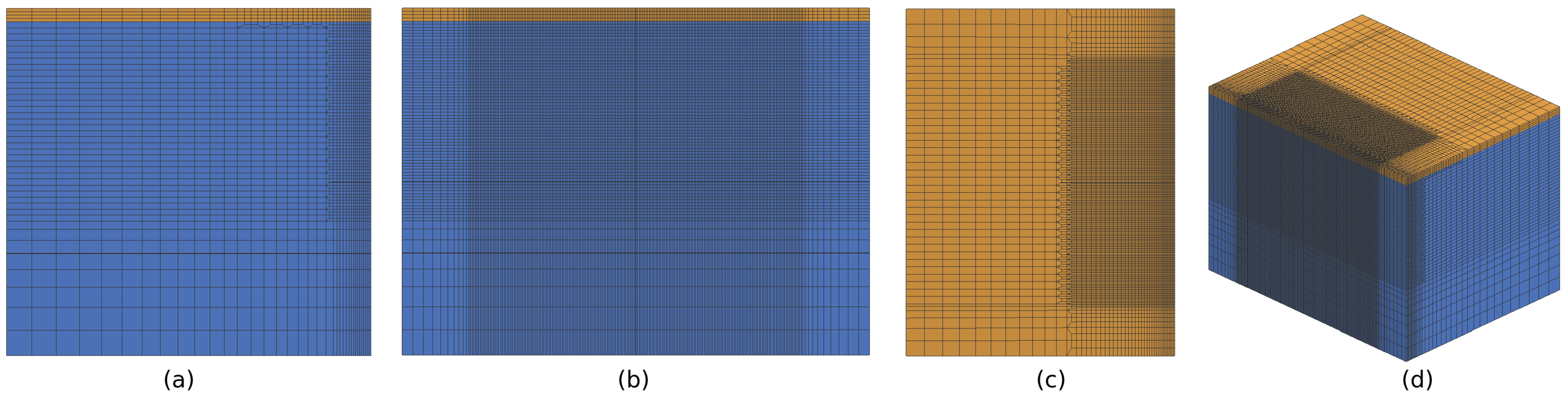
2.2. FE Models and Meshes

Figure 3 and Figure 4 show the FE meshes for SLM AlSi10Mg and SLM Inconel 718, respectively. Mesh refinement only appears along the trajectory of the heat source, and the minimum element size in the substrate is $5\left(length\right)\times 5\left(width\right)\times 9\left(depth\right)$$\mathsf{\mu }$m.

Figure 5 shows the material properties of AlSi10Mg and Inconel 718. Since the experiments of Sadowski et al. [32] and Liu et al. [33] are used as references, therefore, the thicknesses of the powder layer are 20 $\mathsf{\mu }$m for AlSi10Mg and 40 $\mathsf{\mu }$m for Inconel 718. The apparent heat capacity method is employed for Inconel 718 to incorporate the latent heat (L = 210 $\mathrm{kj}\ast {\mathrm{kg}}^{-1}$) due to the phase changing between solid and liquid [37]. The substrate material properties of Al2024 used in SLM AlSi10Mg are exactly the same as Liu et al. [33]. For the sake of convergence, the thermal conductivity of powder varies linearly from 20 degrees to temperature fusion. The thermal properties of powder at ambient temperature (20 degrees) are calculated from the technique presented by Loh et al. [11], and the effective properties of powder are described by the following equations:

$${\rho }_{powder}=(1-\Phi ){\rho }_{compact}$$

(3)

$$K_{powder}=\left\{\begin{array}{cc}{K}_{compact}{(1-\Phi )}^n\hfill & \mathrm{if}T=20\mathrm{degrees}\hfill \\ {\displaystyle \frac{K_{compact}-K_{compact}{(1-\Phi )}^n}{T_{melting}-20}}\ast (T-20)\hfill & \mathrm{otherwise}\hfill \\ K_{compact}\hfill & \mathrm{if}T>T_{melting}\hfill \end{array}\right.$$

(4)

where $\Phi$ is the porosity of powder. In this study, values of $\Phi =0.25$ and $n=4$ are taken [11].

Since the pure heat transfer model has neglected fluid flow in melt pool and multi-physics problems related to the keyhole (see Figure 6), which leads to an under-estimation of molten pool depth and over-estimation of molten pool width, in the literature, the anisotropic thermal conductivity technique has been reported to be useful to improve the precision of molten pool dimensions. This technique has been used to simulate deep penetration by multiplying thermal conductivity by an enhancement factor [33,38,39], as shown in Equation (5).

$$\begin{array}{c}{\mathrm{K}}_{\mathrm{xx}}={\lambda }_{\mathrm{xx}}·\mathrm{k}\hfill \\ {\mathrm{K}}_{\mathrm{yy}}={\lambda }_{\mathrm{yy}}·\mathrm{k}\hfill \\ {\mathrm{K}}_{\mathrm{zz}}={\lambda }_{\mathrm{zz}}·\mathrm{k}\hfill \end{array}$$

(5)

where ${\mathrm{K}}_{\mathrm{xx}},{\mathrm{K}}_{\mathrm{yy}}$, ${\mathrm{K}}_{\mathrm{zz}}$ represent the thermal conductivity in each direction. ${\lambda }_{\mathrm{xx}}$, and ${\lambda }_{\mathrm{yy}}$ and ${\lambda }_{\mathrm{zz}}$ are the temperature-dependant enhancement factors of $\mathrm{k}$ (presented in Table 5).

The depending temperature ($T_c$) and the numerical value of (M) should be estimated and validated from experiments. The enhancement factors are defined according to the following equation:

$$\begin{array}{c}{\lambda }_{\mathrm{xx}}={\lambda }_{\mathrm{yy}}={\lambda }_{\mathrm{zz}}=1,{\mathrm{T}}_1<T_c\hfill \\ {\lambda }_{\mathrm{xx}}={\lambda }_{\mathrm{yy}}=1,{\lambda }_{\mathrm{zz}}=M,{\mathrm{T}}_1\ge T_c\hfill \end{array}$$

(6)

where $T_c$ is greater than temperature fusion and M is generally set to 2–30 [40]. The melt pool depth is supposed to be in the z direction. Liu et al. [33] reported that values of $T_c=750$ degrees and $M=15$ give a good correlation with experiments in SLM AlSi10Mg; therefore, the same values are used in the present study.

However, the enhanced factors are calculated by comparing the predicted values with the experimental results, which is quite complex and time consuming. Moreover, a sharp evolution of thermal conductivity with temperature in one direction would probably lead to a difficulty in convergence.

The principle of simulating deep penetration was inspired by the 3D volumic heat source. The model we proposed is capable of increasing the parameter of penetration automatically in the heat source equation to consider the neglected transport phenomena in the melt pool, and the energy re-distribution in the depth direction related to the keyhole is represented by introducing a parameter that defines the position of maximal power in the depth direction. More details are presented in Section 2.3.

2.3. Heat Source Modeling

Considering the interactions between the powder and laser, the laser penetration depth $\eta$ is generally equal to the thickness of the powder layer. Therefore, the 3D Gaussian heat source is represented as

$$\mathrm{q}(\mathrm{x},\mathrm{y},\mathrm{z})=\left\{\begin{array}{cc}\frac{2\lambda \mathrm{P}}{\pi {r_0}^2\eta }exp\left[-2\frac{r^2}{{r_0}^2}\right]exp\left(-\frac{\left|\mathrm{z}\right|}{\eta }\right);\hfill & \mathrm{if}z\le \eta \mathrm{and}r\le r_0\hfill \\ 0;\hfill & \mathrm{otherwise}\hfill \end{array}\right.$$

(7)

where $r_0$, $\lambda$, P, r, and z are, respectively, the laser beam radius, energy absorptivity, laser power, the distance between the beam center and the point, and the distance from the top surface.

In case of deep penetration, since the governing Equation (1) neglects the fluid flow within the melt pool and the effects of the keyhole (see Figure 6), the melt pool size simulated with the Gaussian heat source described by Equation (7) will therefore under-estimate the penetration and over-estimate the width.

We can start with a comprehensive analysis related to these neglected effects.

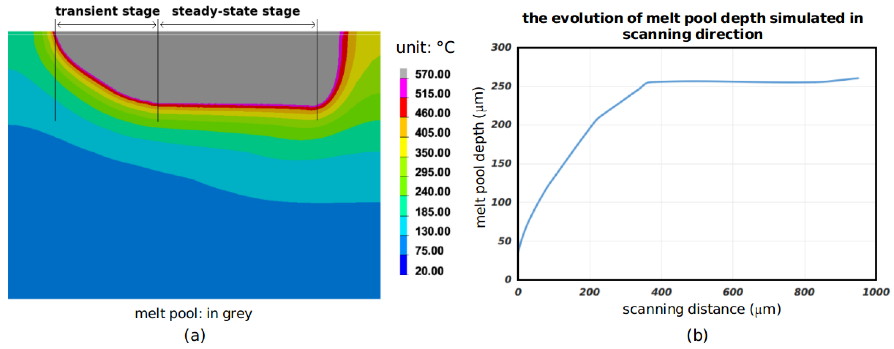
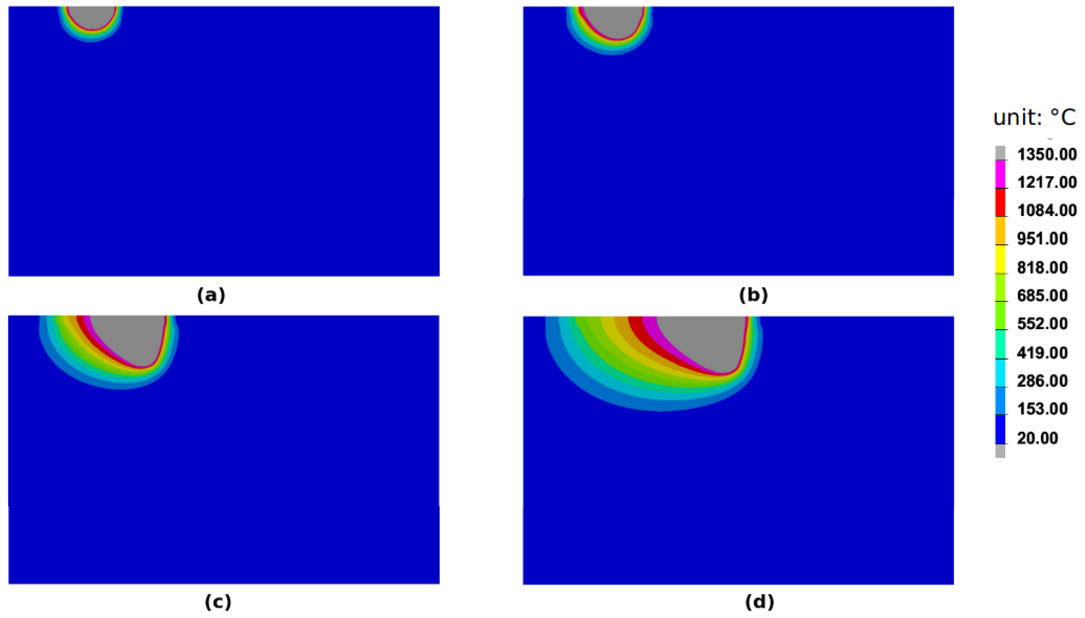
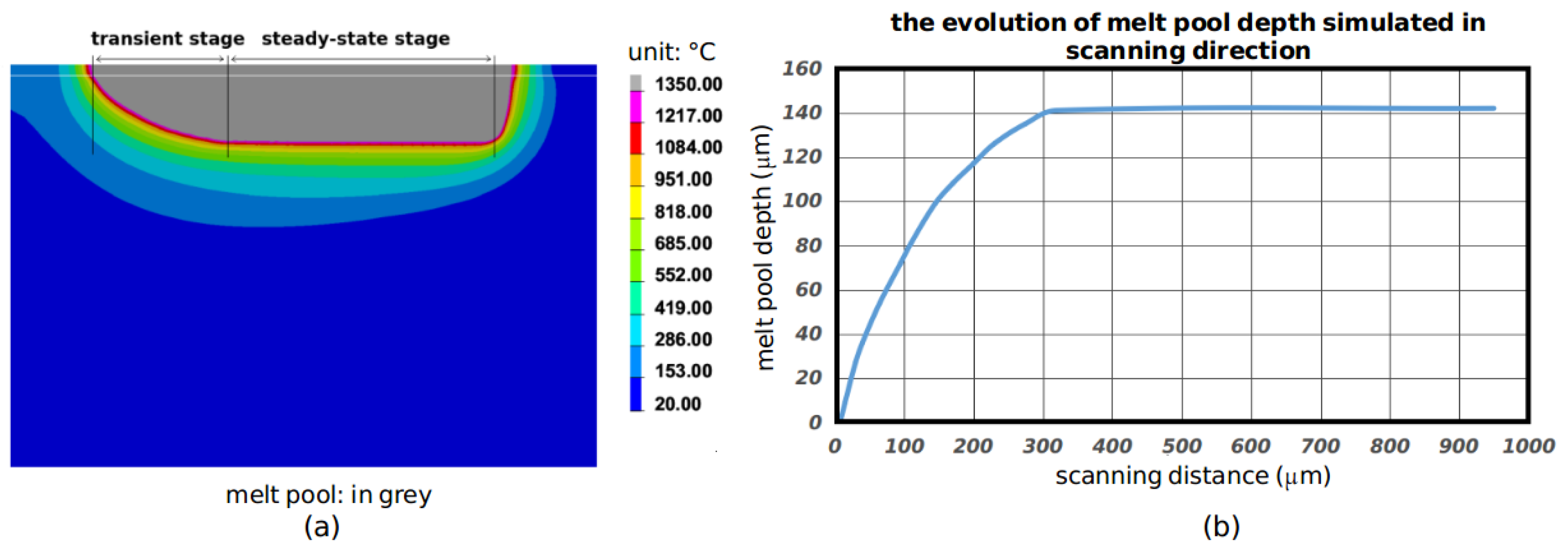
• The fluid flow within the melting pool (Figure 6a) can lead to a more homogeneous temperature distribution by transporting the received energy with the mass flow. Therefore, the anisotropic thermal conductivity technique is well suited to consider the transport effect. In case of high energy input, higher-temperature fluid from the surface heated by a laser is carried toward the bottom of the melt pool [41], which results in a deep-penetration region in the central melt pool. Thus, we propose to increase the parameter $\eta$ to simulate the penetration. Since $\eta$ evolves at each time step, ${\eta }_t$ is now used in Equation (8).
• The effect of multiple reflections on the keyhole (Figure 6b) has been studied by Han et al. [42]. This effect changes the energy distribution in depth, and the maximal power is no longer present at the top surface, which can lead to deeper penetration. One should note that this effect cannot be represented by imposing an enhancement factor for conductivity. The energy distribution described by Equation (7) should be modified by replacing $exp\left(-\frac{\left|\mathrm{z}\right|}{\eta }\right)$ by $exp\left(-\frac{|\mathrm{z}-z_0|}{{\eta }_t}\right)$, where $z_0$ represents the position of maximal power in the depth direction. This parameter is not a fixed value due to the instability of the keyhole, and it is impossible to measure this value from experiments at the moment. Therefore, we propose $z_0$, which is proportional to ${\eta }_t$, for simplicity.

To conclude, the thermal effects related to Figure 6a can be compensated by increasing the parameter of ${\eta }_t$, while ${\eta }_t$ cannot be superior to the melt pool depth. The ${\eta }_t$ is calculated in an explicit manner, where ${\eta }_t$ is updated based on the average temperature of controlled volume (see Figure 7) calculated from instant $t-dt$. The effect of multiple reflection (Figure 6b) can be represented by employing $exp\left(-\frac{|\mathrm{z}-z_0|}{{\eta }_t}\right)$ in Equation (8), and the melt pool depth will be equally enhanced.

In order to ensure a constant energy input as well as consider the variation of ${\eta }_t$ and $z_0$, Equation (7) is transformed into the following form:

$$\mathrm{q}(\mathrm{x},\mathrm{y},\mathrm{z})=\left\{\begin{array}{cc}\frac{2N\lambda \mathrm{P}}{\pi {r_0}^2{\eta }_t}exp\left[-2\frac{r^2}{{r_0}^2}\right]exp\left(-\frac{|\mathrm{z}-z_0|}{{\eta }_t}\right)\hfill & ;\mathrm{if}\mathrm{z}\mathrm{not}\mathrm{greater}\mathrm{than}\eta \hfill \\ 0\hfill & ;\mathrm{otherwise}\hfill \end{array}\right.$$

(8)

where N is recalculated at the beginning of each time step to ensure a constant energy input, and ${\eta }_t$ is also recomputed at beginning of each time step according to the average temperature calculated from selected nodes. We now focus on the procedure of calculating ${\eta }_t$, and this computation is achieved in two steps.

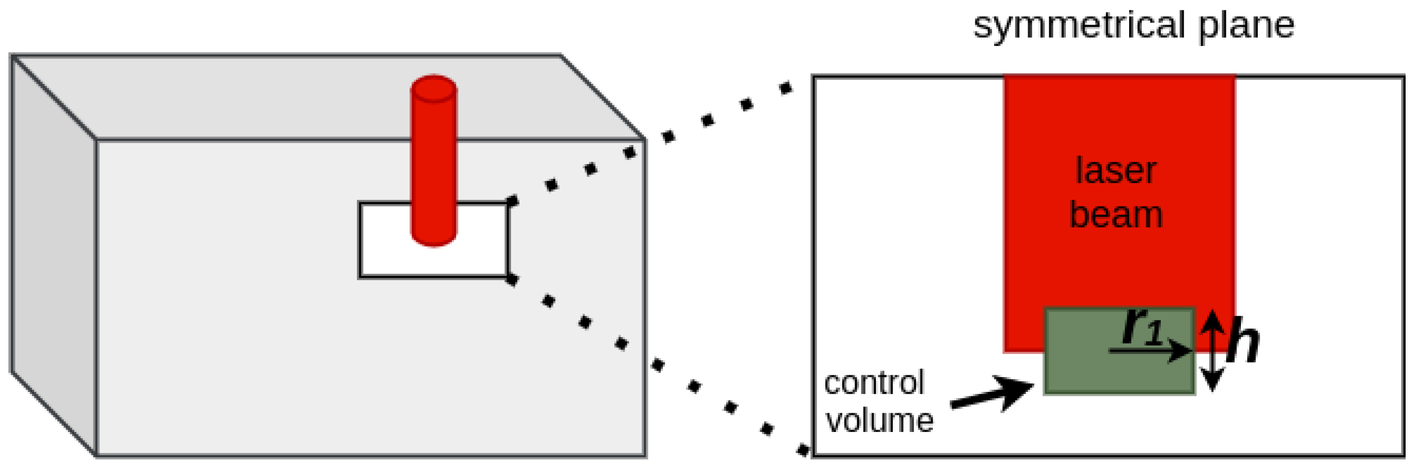
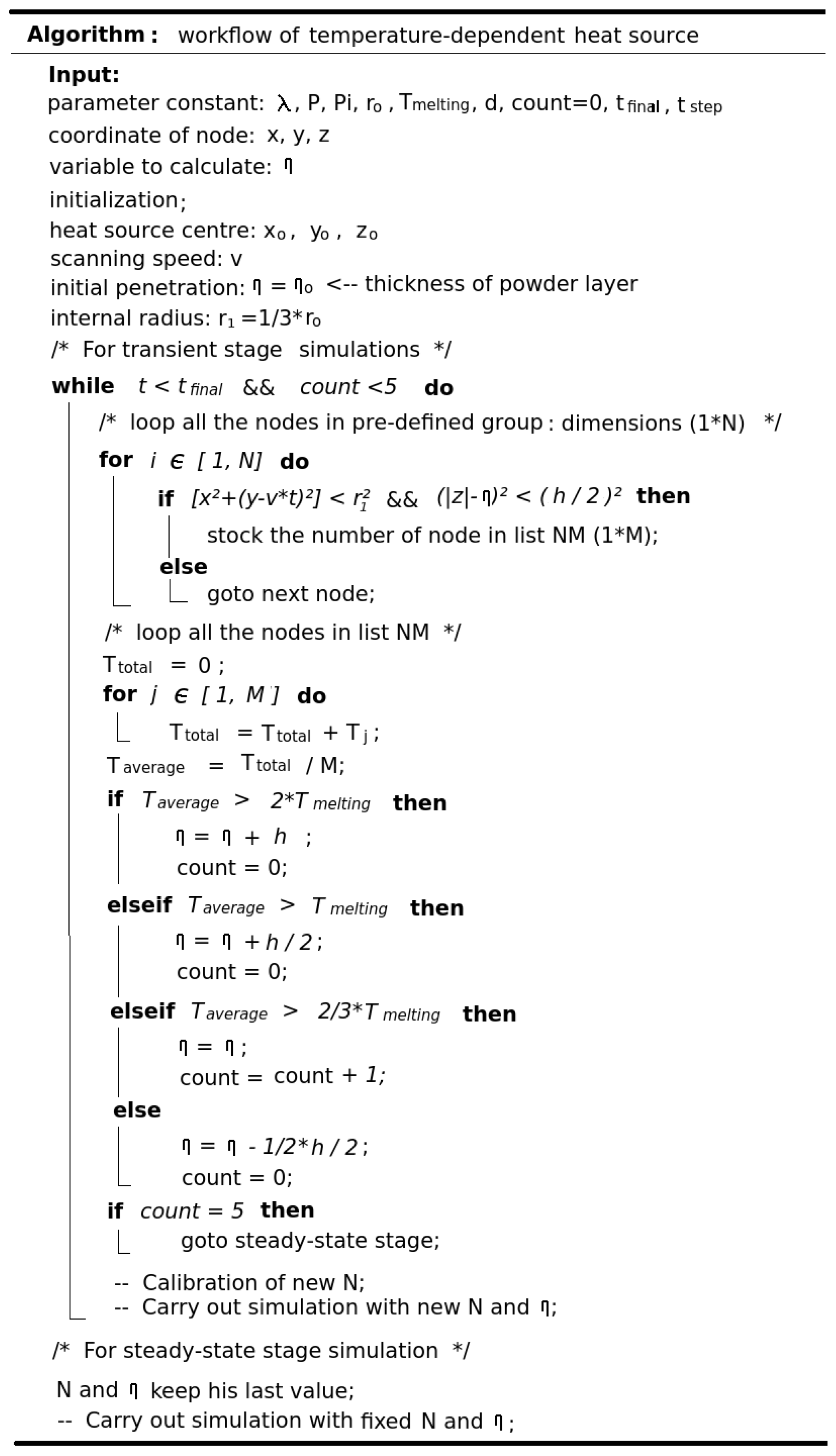
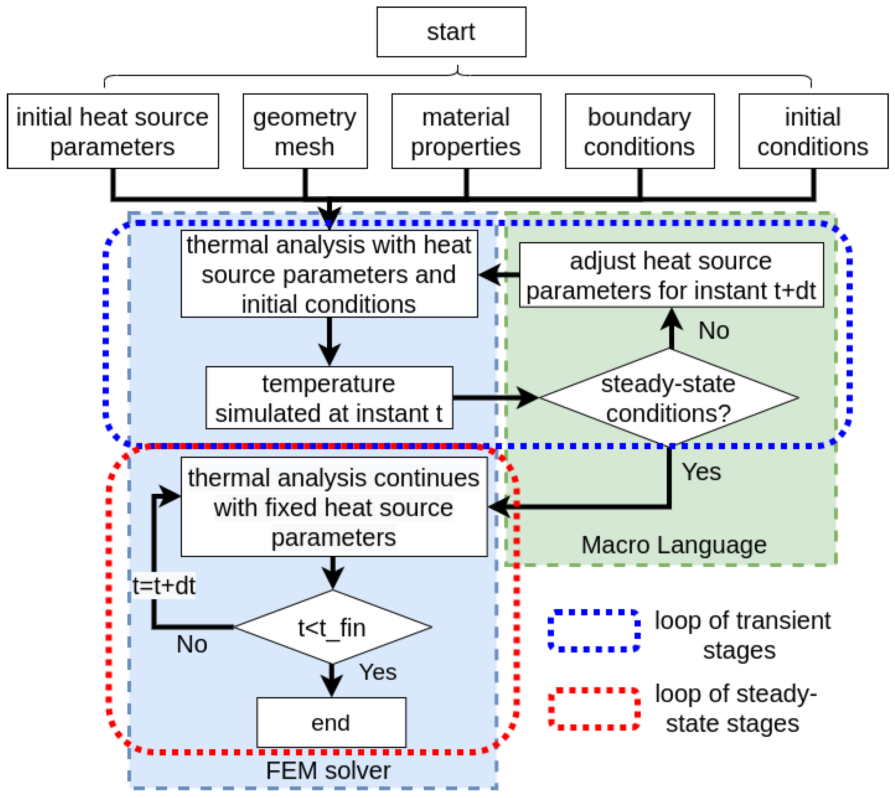
2.3.1. Step 1: Node Selection Procedure

$r_0$ represents the radius of the laser beam. $r_1$ is is set to $\frac{1}{3}{r}_0$, since more than 50% of the energy is distributed within this small area. If we take the moment $t_0$ as example, the center and height of the heat source are $(0,y_{t_0},0)$ and ${\eta }_{t_0}$. A control volume of cylindrical shape is defined by $r_1,h$ and the center of the cylinder (0, $y_{t_0}$, ${\eta }_{t_0}$), where $r_1$ is the radius and h represents the height of cylinder (see Figure 7). We calculate an average temperature from all the nodes included in control volume, and this average temperature is used as the criterion for adjusting ${\eta }_t$.

Figure 8 shows the general procedure for selecting the nodes. A program (SIL) will loop on all the nodes present on the laser path, and the selected nodes should satisfy two conditions: (i) $x^2+{(y-y_{t_0})}^2⩽r_1^2$; (ii) $\left(\right|z|-{\eta }_{t_0}{)}^2⩽{(h/2)}^2$, where $(x,y,z)$ are the coordinates of the node. One should note that $h/2$ should be larger than the minimal element size in the depth direction; otherwise, no nodes could be selected for Step 2. However, $h/2$ should not be so large as to induce the instability due to the adjustment of ${\eta }_t$. In this study, h is set to 20 $\mathsf{\mu }$m. Finally, the green nodes shown in Figure 8 are automatically selected for step 2.

Compared to the strategy of selecting only one node at the bottom center of the laser beam, selecting numerous nodes can provide more representative results, and the average temperature is supposed to be less sensitive to oscillations related to time steps.

2.3.2. Step 2: Adjusting the Heat Source Parameters

The average temperature ($T_{average}$) of selected nodes is calculated from the results of the previous time step. Since the parameter ${\eta }_t$ cannot be greater than the melting pool depth, the material melting temperature is used as a criterion.

Figure 9 presents the possible case according to the relationship between $T_{average}$ and $T_{melting}$. The possible cases at instant t are as follows:

(a)

If $T_{average}⩾T_{melting}$, ${\eta }_t$ should be increased for next time step. If $T_{average}⩾2T_{melting}$, ${\eta }_{t+1}={\eta }_t+h$; otherwise, ${\eta }_{t+1}={\eta }_t+h/2$.

(b)

If ${\displaystyle \frac{2}{3}}{T}_{melting}⩽T_{average}⩽T_{melting}$, ${\eta }_{t+1}$ keeps the same value (${\eta }_t$) for the next time step.

(c)

For the case $T_{average}<{\displaystyle \frac{2}{3}}{T}_{melting}$, which means that ${\eta }_{t+1}$ is over-estimated, ${\eta }_{t+1}={\eta }_t-{\displaystyle \frac{1}{4}}h$ for next time step.

Once a new ${\eta }_{t+1}$ is determined, N should be calibrated again to ensure a constant energy input during the process.

Figure 10 shows the pseudocode for controlling the simulation, which is also a summary of the temperature-dependent heat source. The simulations are performed in two stages: (i) the heat source’s parameters are adjusted in the transient stage, and a small time step is used; (ii) the heat source becomes stable in the steady-state stage, and a larger time step can be employed.

Figure 11 provides an overview of the flowchart of the proposed modeling flow of the SLM process. One should note that steady-state conditions require the same heat source parameters in N successive transient stages to be obtained, and we take $N=5$ in this study. In this article, $SYSWEL{D}^{TM}$ software and its Marco language $SIL$ are used to implement the proposed heat source. The same procedure can also be achieved using other software and Macro languages, such as Python for Abaqus and APDL for Ansys.

3. Results and Discussions

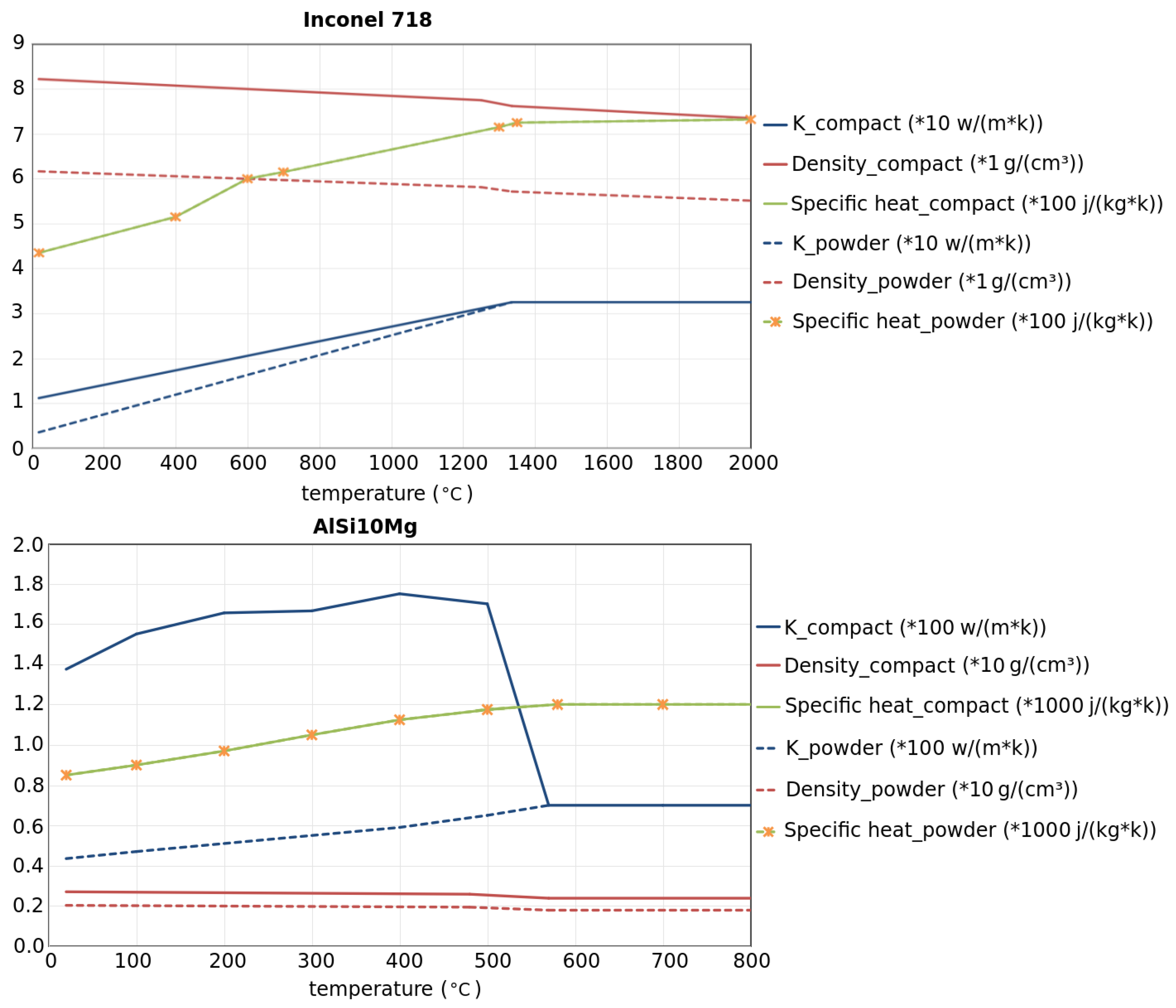
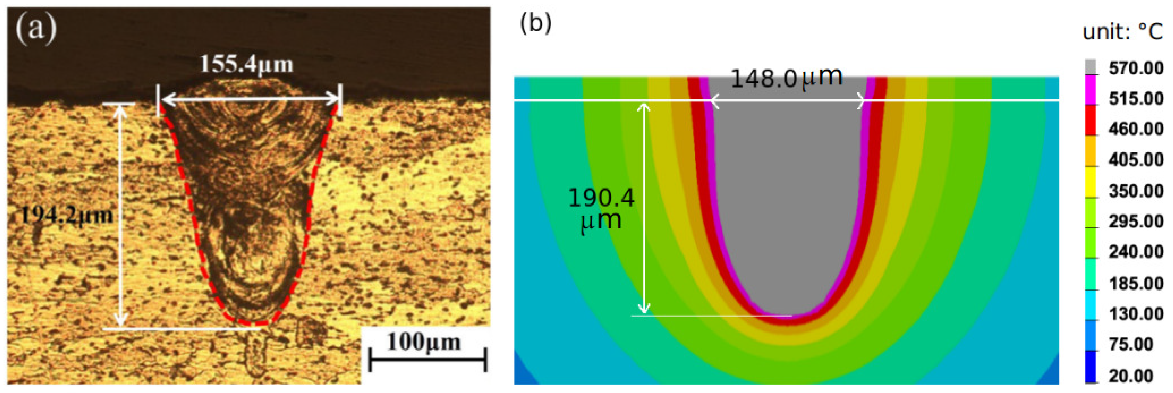
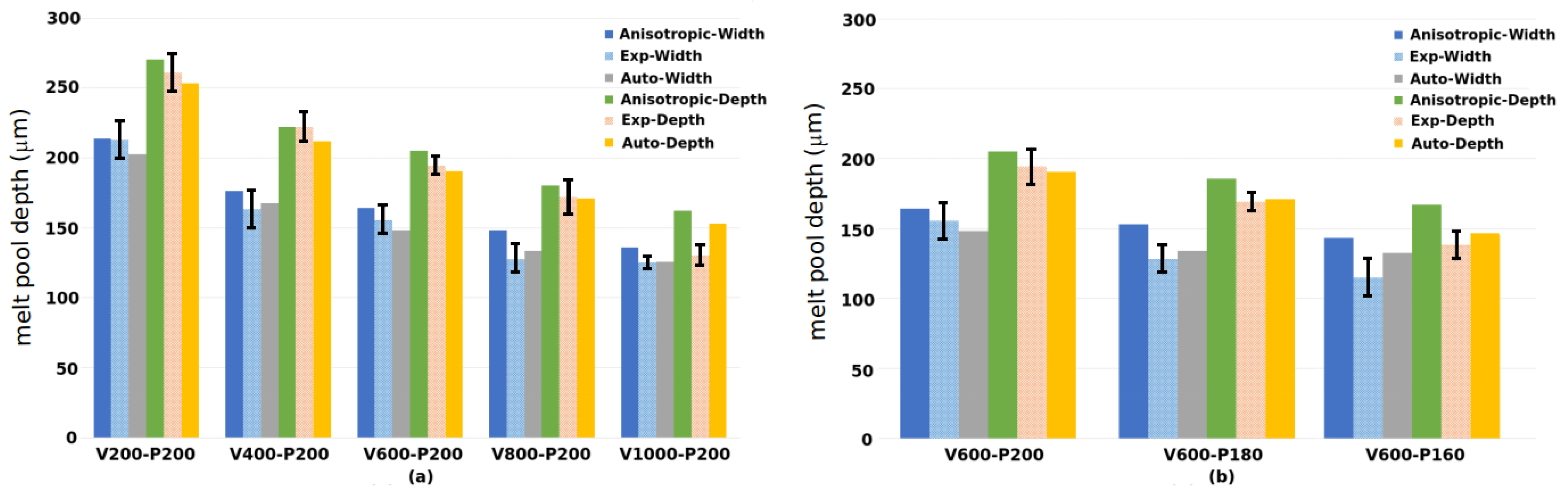
The melt pool width and depth are illustrated in Figure 12, and both experimental results and numerical results are measured in the same way. To ensure the good stability of prediction during the transient stage, a time step of smaller than ${\displaystyle \frac{r_0}{3\ast V_{scanning}}}$ is recommended. FE software $SYSWELD$ [43] was utilized to model SLM.

3.1. SLM AlSi10Mg

Table 1. Process parameters used in SLM AlSi10 Mg [33].

Sample No.	1 #	2 #	3 #	4 #	5 #	6 #	7 #
Scanning speed (mm/s)	200	400	600	800	1000	600	600
Laser power (W)	200	200	200	200	200	180	160
Beam radius ($\mathsf{\mu }$m)	50
Layer thickness ($\mathsf{\mu }$m)	20
Absortivity	0.6
Initial temperature (°C)	25

presents the scanning speed and laser power applied in SLM simulations. The other parameters, such as emissivity, coefficient exchange, initial conditions, and so on are the same as those used by Liu et al. [33]. The experimental results of sample $1\#$ are used to calibrate $z_0$ ($z_0=0.66\ast {\eta }_t$). The simulation results of V200-P200 (scanning speed labeled V: 200 mm/s and laser power labeled P: 200 Watt) are used to illustrate certain characters of the proposed heat source.

Figure 13 shows the melting pool shape at different moments during the simulation, and the contours are shown at the symmetrical plane. The melting pool depth increases progressively over time, since the heat source increases its penetration automatically.

The final simulated melt pool shape is shown in Figure 14, and two stages can be clearly identified. The melt pool depth keeps increasing in the transient stage, while the melt pool depth is almost constant in the steady-state stage. A slight increase of the melt pool depth can be observed in the steady-state stage, which is perhaps due to the boundary effect as the model is short.

Another investigation concerns the sensibility of the time step, as it is known that ${\eta }_t$ is calculated in an explicit way. Figure 15 shows the molten profiles simulated with different time steps, where the maximal recommended time step is $dt={\displaystyle \frac{r_0}{3\ast V_{scanning}}}=0.06$ ms. The comparison of the melt pool depths shows that a temperature-dependent heat source is stable and slightly sensitive to the time step. A maximum difference of $3.8\%$ is observed, and the increase of melt pool depth in dt = 0.125 ms is perhaps due to the boundary effect. Even though the time step is different in this study, the number of time steps required to achieve the steady-state stage is almost the same (about 29 transient time steps).

Figure 16 provides the comparison of the cross-section morphology of three melt pool shapes. The dimensions of the melt pool given by experiment and simulation are quite similar, and the relative error between the experimental and simulated data is $4.8\%$ for width and $2\%$ for depth. One should note that the heat source parameters are adjusted automatically without any manual intervention.

The comparison of the molten pool dimensions of the experimental and numerical results is presented in Figure 17, and good correlations among experimental results (Exp-Width and Exp-Depth) [33], numerical results with the proposed heat source (Auto-Width and Auto-Depth), and with the anisotropic conductivity method (Anisotropic-Width and Anisotropic-Depth) [33] are found. The proposed heat source is capable of predicting the melting pool dimension with different process parameters correctly. Compared to the experimental results, the average relative errors given by the proposed model are generally less than $4.8\%$ for depth and $5.2\%$ for width. A better precision of prediction than the anisotropic conductivity method is thus observed. Moreover, with fixed laser power, both the width and depth of the molten pool decrease if the scanning speed increases. When the scanning speed is fixed at 600 mm/s, the width and depth increase with increasing laser power.

3.2. SLM Inconel 718

We now apply the proposed heat source for the SLM Inconel 718, and the experimental results are taken from Sadowski et al. [32]. The initial parameter ${\eta }_{t=0}$ is equal to 40 $\mathsf{\mu }$m, and $z_0$ is $0.4\ast {\eta }_t$. The reported absorptivity of Inconel 718 varies from 0.3–0.87 [27,44]; therefore, $0.7$ is used in this study. The processing parameters (scanning speed and laser power) used are shown in

Table 2. Scanning speed and laser power in SLM Inconel 718 [32].

Scanning speed (mm/s)	200	200	200	200
Laser power (Watt)	100	150	200	300
Beam radius ($\mathsf{\mu }$m)	37.5
Layer thickness ($\mathsf{\mu }$m)	40
Absorptivity	0.7
Initial temperature (°C)	20

, and other parameters can be found in the work of Romano et al. [27].

Figure 18 presents the melting pool at different moments during the simulation. Compared to the temperature distribution in Figure 13, the heat diffuses very slowly in Inconel 718 because of its low diffusivity.

Figure 19 shows the final simulated molten pool shape (speed: 200 mm/s, power: 100 Watt). The molten pool depth increases in the transient stage and keeps constant in the steady-state stage. Boundary effects become negligible due to low diffusivity. Thus, the melt pool depth in the steady-state stage does not increase as we observed in SLM ALSi10Mg.

Similarly, the effect of the time step is studied in SLM Inconel 718. Figure 20 presents the molten profiles after the SLM process and the variation of melt pool depth in the scanning direction. In the steady-state stage, a maximum difference of $2.9\%$ is observed, and we can conclude that the precision is satisfactory.

Finally, a comparison of the molten pool dimensions given by experiments and numerical simulations is presented in Figure 21. The simulated melt pool depth gives good precision compared to experiments, while the width is slightly under-estimated. Thus, a maximal relative error of $9.6\%$ is found.

The proposed heat source is therefore validated through the comparisons of its results (melt pool morphology for two materials: AlSi10Mg and Inconel 718) with those of the existing numerical method (anisotropic thermal conductivity technique) and experimental tests. Compared to the anisotropic thermal conductivity technique, the procedure of parameter calibration in the proposed heat source (only the parameter $z_0$ must be calibrated) is easier. Moreover, numerical investigation shows that the proposed heat source is slightly sensitive to the choice of the time step. In contrast, a sharp increase of thermal conductivity induced by the anisotropic thermal conductivity technique leads to the difficulty of converging, which results in only very small time steps being applied. The difficulty of converging could be further increased if the metallurgical transformation is considered. Therefore, the proposed heat source is more efficient in terms of computation cost than the anisotropic thermal conductivity technique. Note that the proposed heat source can be subsequently used for other materials and processes (for example, laser welding by the keyhole technique).

4. Conclusions

A thermal model based on a new heat source has been developed to simulate deep penetration during the SLM process. This heat source can adjust its parameters during the simulation to compensate the neglected thermal effects related to the fluid flow and keyhole. Its parameters become fixed once the temperature distribution becomes stable. The proposed model has been validated on experimental results (for two materials: ALSI10Mg and Inconel 718) from the literature. The comparisons of melt pool morphology showed a good correlation between numerical and experimental results.

References

1. Huang, S.H.; Liu, P.; Mokasdar, A.; Hou, L. Additive manufacturing and its societal impact: A literature review. Int. J. Adv. Manuf. Technol. 2013, 67, 1191–1203. [Google Scholar] [CrossRef]
2. Singh, S.; Ramakrishna, S.; Singh, R. Material issues in additive manufacturing: A review. J. Manuf. Process 2017, 25, 185–200. [Google Scholar] [CrossRef]
3. Yan, W.; Smith, J.; Ge, W.; Lin, F.; Liu, W.K. Multiscale modeling of electron beam and substrate interaction: A new heat source model. Comput. Mech. 2015, 56, 265–276. [Google Scholar] [CrossRef]
4. Saadlaoui, Y.; Delache, A.; Feulvarch, E.; Leblond, J.B.; Bergheau, J.M. New strategy of solid/fuid coupling during numerical simulation of welding process. J. Fluids Struct. 2020, 99, 103161. [Google Scholar] [CrossRef]
5. Khairallah, S.A.; Anderson, A. Mesoscopic simulation model of selective laser melting of stainless steel powder. J. Mater. Process. Technol. 2014, 214, 2627–2636. [Google Scholar] [CrossRef]
6. Yan, W.; Ge, W.; Qian, Y.; Lin, S.; Zhou, B.; Liu, W.K.; Lin, F.; Wagner, G.J. Multi-physics modeling of single/multiple-track defect mechanisms in electron beam selective melting. Acta Mater. 2017, 134, 324–333. [Google Scholar] [CrossRef]
7. Bayat, M.; Mohanty, S.; Hattel, J.H. Multiphysics modelling of lack-of-fusion voids formation and evolution in IN718 made by multi-track/multi-layer L-PBF. Int. J. Heat Mass Transf. 2019, 139, 95–114. [Google Scholar] [CrossRef]
8. Saadlaoui, Y.; Feulvarch, E.; Leblond, J.B.; Bergheau, J.M. Numerical Simulation of the Molten Pool of a Powder Bed. In Proceedings of the 14th WCCM-ECCOMAS Congress 2020, Paris, France, 11–15 January 2021; Volume 1000. [Google Scholar] [CrossRef]
9. Saadlaoui, Y.; Feulvarch, E.; Delache, A.; Leblond, J.B.; Bergheau, J.M. A new strategy for the numerical modeling of a weld pool. Comptes Rendus Mécanique 2018, 346, 999–1017. [Google Scholar] [CrossRef]
10. Chen, Q.; Guillemot, G.; Gandin, C.A.; Bellet, M. Numerical modelling of the impact of energy distribution and Marangoni surface tension on track shape in selective laser melting of ceramic material. Addit. Manuf. 2018, 21, 713–723. [Google Scholar] [CrossRef]
11. Loh, L.-E.; Chua, C.-K.; Yeong, W.-Y.; Song, J.; Mapar, M.; Sing, S.-L.; Liu, Z.H.; Zhang, D.Q. Numerical investigation and an effective modelling on the Selective Laser Melting (SLM) process with aluminium alloy 6061. Int. J. Heat Mass Transf. 2015, 80, 288–300. [Google Scholar] [CrossRef]
12. Mukherjee, T.; Wei, H.L.; DebRoy, A.; De, T. Heat and fluid flow in additive manufacturing—Part I: Modeling of powder bed fusion. Comput. Mater. Sci. 2018, 150, 304–313. [Google Scholar] [CrossRef] [Green Version]
13. Le, T.-N.; Lo, Y.-L.; Lin, Z.-H. Numerical simulation and experimental validation of melting and solidification process in selective laser melting of IN718 alloy. Addit. Manuf. 2020, 36, 101519. [Google Scholar] [CrossRef]
14. Lu, X.; Cervera, M.; Chiumenti, M.; Li, J.; Ji, X.; Zhang, G.; Lin, X. Modeling of the Effect of the Building Strategy on the Thermomechanical Response of Ti-6Al-4V Rectangular Parts Manufactured by Laser Directed Energy Deposition. Metals 2020, 10, 1643. [Google Scholar] [CrossRef]
15. Promoppatum, P.; Yao, S.-C. Influence of scanning length and energy input on residual stress reduction in metal additive manufacturing: Numerical and experimental studies. J. Manuf. Process. 2020, 49, 247–259. [Google Scholar] [CrossRef]
16. Huang, H.; Ma, N.; Chen, J.; Feng, Z.; Murakawa, H. Toward large-scale simulation of residual stress and distortion in wire and arc additive manufacturing. Addit. Manuf. 2020, 34, 101248. [Google Scholar] [CrossRef]
17. Bock, F.E.; Herrnring, J.; Froend, M.; Enz, J.; Kashaev, N.; Klusemann, B. Experimental and numerical thermo-mechanical analysis of wire-based laser metal deposition of Al-Mg alloys. J. Manuf. Process. 2021, 64, 982–995. [Google Scholar] [CrossRef]
18. Dal, M.; Fabbro, R. An overview of the state of art in laser welding simulation. Opt. Laser Technol. 2016, 78, 2–14. [Google Scholar] [CrossRef] [Green Version]
19. Rosenthal, D. Mathematical theory of heat distribution during welding and cutting. Weld. J. 1941, 20, 220–234. [Google Scholar]
20. Ning, J.; Mirkoohi, E.; Dong, Y.; Sievers, D.E.; Garmestani, H.; Liang, S.Y. Analytical modeling of 3D temperature distribution in selective laser melting of Ti-6Al-4V considering part boundary conditions. J. Manuf. Process. 2019, 44, 319–326. [Google Scholar] [CrossRef]
21. Ning, J.; Wang, W.; Zamorano, B.; Liang, S.Y. Analytical modeling of lack-of-fusion porosity in metal additive manufacturing. Appl. Phys. A 2019, 125, 797. [Google Scholar] [CrossRef]
22. Ning, J.; Sievers, D.; Garmestani, H.; Liang, S. Analytical Modeling of Part Porosity in Metal Additive Manufacturing. Int. J. Mech. Sci. 2020, 172, 105428. [Google Scholar] [CrossRef]
23. Wang, W.; Ning, J.; Liang, S.Y. In-Situ Distortion Prediction in Metal Additive Manufacturing Considering Boundary Conditions. Int. J. Precis. Eng. Manuf. 2021, 22, 909–917. [Google Scholar] [CrossRef]
24. Lu, X.; Lin, X.; Chiumenti, M.; Cervera, M.; Hu, Y.; Ji, X.; Ma, L.; Huang, W. In situ measurements and thermo-mechanical simulation of Ti-6Al-4V laser solid forming processes. Int. J. Mech. Sci. 2019, 153, 119–130. [Google Scholar] [CrossRef]
25. Fu, C.H.; Guo, Y.B. Three-Dimensional Temperature Gradient Mechanism in Selective Laser Melting of Ti-6Al-4V. ASME J. Manuf. Sci. Eng. 2014, 136, 061004. [Google Scholar] [CrossRef]
26. Romano, J.; Ladani, L.; Sadowski, M. Thermal modeling of laser based additive manufacturing processes within common materials. Procedia Manuf 2015, 1, 238–250. [Google Scholar] [CrossRef] [Green Version]
27. Romano, J.; Ladani, L.; Sadowski, M. Laser additive melting and solidification of Inconel 718: Finite element simulation and experiment. JOM 2016, 68, 967–977. [Google Scholar] [CrossRef]
28. Lu, X.; Zhang, G.; Li, J.; Cervera, M.; Chiumenti, M.; Chen, J.; Lin, X.; Huang, W. Simulation-assisted investigation on the formation of layer bands and the microstructural evolution in directed energy deposition of Ti6Al4V blocks. Virtual Phys. Prototyp. 2021, 16, 387–403. [Google Scholar] [CrossRef]
29. Lu, X.; Chiumenti, M.; Cervera, M.; Tan, H.; Lin, X.; Wang, S. Warpage Analysis and Control of Thin-Walled Structures Manufactured by Laser Powder Bed Fusion. Metals 2021, 11, 686. [Google Scholar] [CrossRef]
30. Promoppatum, P.; Yao, S.-C.; Pistorius, P.C.; Rollett, A.D. A Comprehensive Comparison of the Analytical and Numerical Prediction of the Thermal History and Solidification Microstructure of Inconel 718 Products Made by Laser Powder-Bed Fusion. Engineering 2017, 3, 685–694. [Google Scholar] [CrossRef]
31. Walker, T.R.; Bennett, C.J. An automated inverse method to calibrate thermal finite element models for numerical welding applications. J. Manuf. Process. 2019, 47, 263–283. [Google Scholar] [CrossRef]
32. Sadowski, M.; Ladani, L.; Brindley, W.; Romano, J. Optimizing quality of additively manufactured Inconel 718 using powder bed laser melting process. Addit. Manuf. 2016, 11, 60–70. [Google Scholar] [CrossRef]
33. Liu, S.; Zhu, H.; Peng, G.; Yin, J.; Zeng, X. Microstructure prediction of selective laser melting AlSi10Mg using finite element analysis. Mater. Des. 2018, 142, 319–328. [Google Scholar] [CrossRef]
34. Feulvarch, E.; Roux, J.-C.; Bergheau, J.-M. Theoretical Framework of a Variational Formulation for Nonlinear Heat Transfer with Phase Changes. Math. Probl. Eng. 2013, 2013, 257104. [Google Scholar] [CrossRef] [Green Version]
35. Proell, S.D.; Wall, W.A.; Meier, C. On phase change and latent heat models in metal additive manufacturing process simulation. Adv. Model. Simul. Eng. Sci. 2020, 7, 1–32. [Google Scholar] [CrossRef]
36. Bergheau, J.-M.; Rol, F. Finite Element Simulation of Heat Transfer; John Wiley & Sons: Hoboken, NJ, USA, 2013. [Google Scholar]
37. Bonacina, C.; Comini, G.; Fasano, A.; Primicerio, M. Numerical solution of phasechange problems. Int. J. Heat Mass Transfer. 1973, 16, 1825–1832. [Google Scholar] [CrossRef]
38. Kamara, A.M.; Wang, W.; Marimuthu, S.; Li, L. Modelling of the melt pool geometry in the laser deposition of nickel alloys using the anisotropic enhanced thermal conductivity approach. Proc. Inst. Mech. Eng. B J. Eng. Manuf. 2011, 225, 2341–2344. [Google Scholar] [CrossRef]
39. Trapp, J.; Rubenchik, A.M.; Guss, G.; Matthews, M.J. In situ absorptivity measurements of metallic powders during laser powder-bed fusion additive manufacturing. Appl. Mater. Today 2017, 9, 341–349. [Google Scholar] [CrossRef]
40. Zhang, Z.; Huang, Y.; Kasinathan, A.R.; Shahabad, S.I.; Ali, U.; Mahmoodkhani, Y.; Toyserkani, E. 3-Dimensional heat transfer modeling for laser powder-bed fusion additive manufacturing with volumetric heat sources based on varied thermal conductivity and absorptivity. Opt. Laser Technol. 2019, 109, 297–312. [Google Scholar] [CrossRef]
41. Gan, Z.; Yu, G.; He, X.; Li, S. Surface-active element transport and its effect on liquid metal flow in laser-assisted additive manufacturing. Int. Commun. Heat. Mass Transf. 2017, 86, 206–214. [Google Scholar] [CrossRef] [Green Version]
42. Han, S.W.; Ahn, J.; Na, S.J. A study on ray tracing method for CFD simulations of laser keyhole welding: Progressive search method. Weld World 2016, 60, 247–258. [Google Scholar] [CrossRef]
43. Software SYSWELD Version 2020; ESI-Group: Lyon, France, 2020.
44. Sainte-Catherine, C.; Jeandin, M.; Kechemair, D.; Ricaud, J.P.; Sabatier, L. Study of dynamic absorptivity at 10.6 μm (CO2) and 1.06 μm (Nd-YAG) wavelengths as a function of temperature. J. Phys. IV Fr. 1991, 1, C7-151–C7-157. [Google Scholar] [CrossRef] [Green Version]
Figure 1. Example of thermo-mechanical simulation.
Applsci 11 11406 g001
Figure 2. Dimensions of model and schematic diagram of thermal behavior in SLM process.
Applsci 11 11406 g002
Figure 3. FE mesh (286,196 nodes/271,034 3D elements) for SLM AlSi10Mg: left view (a); front view (b); top view (c); global view (d).
Applsci 11 11406 g003
Figure 4. FE mesh (450,133 nodes/430,570 3D elements) for SLM Inconel 718: left view (a); front view (b); top view (c); global view (d).
Applsci 11 11406 g004
Figure 5. The temperature-dependent material properties used in this study.
Applsci 11 11406 g005
Figure 6. Thermal effects neglected by FEM: fluid flow (a); multiple reflections due to keyhole (b).
Applsci 11 11406 g006
Figure 7. Schematic diagram of the control volume.
Applsci 11 11406 g007
Figure 8. Schematic diagram of node selection.
Applsci 11 11406 g008
Figure 9. Diagram of possible cases.
Applsci 11 11406 g009
Figure 10. Pseudocode for calculation of heat source parameters.
Applsci 11 11406 g010
Figure 11. Flowchart of the proposed modeling flow.
Applsci 11 11406 g011
Figure 12. Schematic diagram to illustrate the sizes of the molten pool.
Applsci 11 11406 g012
Figure 13. Melting pool shape simulated in SLM AlSi10Mg (V200-P200) at t = 0.1 ms (a); t = 0.5 ms (b); t = 1 ms (c); t = 1.5 ms (d).
Applsci 11 11406 g013
Figure 14. Final melt pool depth simulated in SLM AlSi10Mg (V200-P200) (a) and the evolution of melt pool depth in scanning direction (b).
Applsci 11 11406 g014
Figure 15. Investigation of effect of time step (0.050 ms, 0.075 ms, 0.100 ms, 0.125 ms) in SLM AlSi10Mg (V200-P200): melt pool depth in the symmetrical plane (a) and comparison of the evolution of melt pool depth simulated for different time steps (b).
Applsci 11 11406 g015
Figure 16. The melt pool of SLM AlSi10Mg (V600-P200) experimental model (a) [33] and numerical model (b).
Applsci 11 11406 g016
Figure 17. Comparison of molten pool dimensions given by experiments [33] and numerical simulations: fixed laser power of 200 Watt (a) and fixed scanning speed of 600 mm/s (b).
Applsci 11 11406 g017
Figure 18. Melt pool shape in SLM Inconel 718 (V200-P100) at t = 0.15 ms (a); t = 0.35 ms (b); t = 1 ms (c); t = 2 ms (d).
Applsci 11 11406 g018
Figure 19. Final simulated molten pool shape in SLM Inconel 718 (V200-P100) (a) and the evolution of melt pool depth in scanning direction (b).
Applsci 11 11406 g019
Figure 20. Investigation of effect of time step (0.050 ms, 0.075 ms, 0.100 ms, 0.125 ms) in SLM Inconel 718 (V200-P100): melt pool depth in the symmetrical plane (a) and comparison of the evolution of melt pool depth simulated for different time steps (b).
Applsci 11 11406 g020
Figure 21. Comparison of molten pool dimensions given by experiments [32] and numerical simulations: fixed scanning speed of 200 mm/s.
Applsci 11 11406 g021