Abstract
The small and transparent nematode Caenorhabditis elegans is increasingly employed for phenotypic in vivo chemical screens. The influence of compounds on worm body fat stores can be assayed with Nile red staining and imaging. Segmentation of C. elegans from fluorescence images is hereby a primary task. In this paper, we present an image-processing workflow that includes machine-learning-based segmentation of C. elegans directly from fluorescence images and quantifies their Nile red lipid-derived fluorescence. The segmentation is based on a J48 classifier using pixel entropies and is refined by size-thresholding. The accuracy of segmentation was >90% in our external validation. Binarization with a global threshold set to the brightness of the vehicle control group worms of each experiment allows a robust and reproducible quantification of worm fluorescence. The workflow is available as a script written in the macro language of imageJ, allowing the user additional manual control of classification results and custom specification settings for binarization. Our approach can be easily adapted to the requirements of other fluorescence image-based experiments with C. elegans.
1. Introduction
Caenorhabditis elegans is a 1 mm sized, plain, transparent roundworm and represents a promising model for phenotype directed screening [1,2,3]. It is widely used for the identification of genes and chemicals that regulate fat storage, as key mammal fat-regulatory genes and pathways are conserved in the worm [4,5]. In recent years great efforts have been made to study the fat metabolism of C. elegans. Several methods have been described to quantify lipid content in worms [6,7]. C. elegans stores lipids differently than mammals. Nematodes have neither adipocytes nor a liver-like organ. Triacyl glycerides (TAG) are stored in the intestine and epidermis in lipid droplets, lysosome-related organelles, and the yolk [4]. The latter is transported to the germline, which also deposits a considerable amount of lipids [8].
Whole organism lipids can be extracted and later analyzed by chromatographic techniques or biochemical assays [9]. Because of the worm’s transparent body, GFP fusion proteins as markers for lipid-rich particles, like the yolk (VIT-2::GFP) and lipid droplets (DHS-3::GFP), are reported [10,11]. Label-free imaging techniques such as spectroscopic coherent Raman [12] and coherent anti-Stokes Raman scattering imaging [13,14] are important tools for C. elegans lipid-storage studies, but require expensive equipment. The most commonly used technique is histochemical staining, e.g., with Oil Red O [15,16] or the solvatochromatic dye Nile red [17,18,19]. There are controversial opinions on which stains and methodologies are best suited for lipid content quantification [4,12,15]. O’Rourke and coworkers pointed out that vital Nile red stains lysosome-related organelles of the intestine and not neutral lipid stores [15]. Because the vital Nile red fluorescence intensity increases during short-term starvation [20], Lemieux and coworkers [4] suggested that Nile-red-stained organelles function as normal lipid reservoir junctions and increase accordingly during lipid mobilization. Whole body lipid staining has also been questioned in general by the observation that most intestinal lipid particles are yolk or serve yolk production and are not energy reservoirs orthologous to mammals [12]. Despite all these considerations, Nile red staining brings several advantages, particularly its fast and easy application and its good sensitivity [4].
We have recently established a miniaturized fat accumulation assay in 96-well plates based on the staining of lipid compartments with Nile red [21]. For the efficient quantitation of lipid-derived fluorescence of worms, an image processing workflow capable of segmenting worms from fluorescence microscopy images was necessary.
In the field of image processing, assigning a pixel to either the region of interest—such as the worm—or to the background, is called segmentation. Because manual segmentation is time-consuming and dependent on researchers and their constitution [22], great efforts have been made for automating the segmentation procedures of microscopical images of C. elegans [23,24,25]. There are several well-established procedures for the segmentation of C. elegans on brightfield images. The online tool IPPOME accurately segments images of worms on agar pads by noise-reduction and the Chan–Vese algorithm [16]. The wormachine is a MATLAB-based image analysis tool which incorporates worm segmentation from agar brightfield images by auto-thresholding. Objects are then identified as worms by a size thresholding step and a convolutional neural network [26]. The wormsizer is an imageJ plugin for the segmentation and size measurement of C. elegans brightfield images. After image preprocessing to remove uneven illumination, segmentation is performed with a simple global thresholding approach refined by size-filters [27]. Fudickar, Bornhorst, and coworkers [28,29] have successfully trained machine-learning classifiers for brightfield images from agar plates obtained by do-it-yourself microscopes using smartphones or Raspberry Pi camera modules. The wormtoolbox [30], available through cellprofiler [31], can be used for static brightfield images of adult worms in liquid culture. In this process, segmentation is performed by binarization with Otus’s thresholding. Afterwards, objects are identified as worms by a model using shape descriptors retrieved from object skeletons. This tool also enables the disentanglement of touching worms for individual worm segments [30]. There are also some procedures described for the segmentation and processing of Nile red fluorescence images. Escorcia and coworkers [32] have reported a very detailed description of quantifying Nile red fluorescence from worms on microscope slide images, but their method is highly handcrafted, e.g., by manual segmentation of the worms.
Hence, to quantify the fluorescence of individual worms, it is necessary to record both brightfield as well as fluorescence images. Segmentation into region of interest (the worms) and background is calculated using the reported procedures in the brightfield channel. The segmentation results can then be used as a mask for the actual fluorescence images [30,33,34]. However, acquiring brightfield images of worms in 96-well liquid culture in addition to fluorescence images can cause problems, such as poor segmentation due to illumination variations at the well edges or fluorescence bleaching; other requirements, such as an increased amount of hard disk space and an increased recording time, must also be considered.
Our fluorescence images allowed for the easy recognition of worms by operators; they also enabled operators to manually distinguish C. elegans from background signals derived from, e.g., bacteria or precipitates. Therefore, the goal was to develop a new, simple, and automated image processing workflow which does not require brightfield images for segmentation. Our final workflow in this study is shown in Figure 1 and comprises (1) the adjustment of contrast and brightness of the fluorescence images, (2) classification into worm and background, (3) refinement by particle-size thresholding, (4) segmentation, and (5) binarization of images for quantitation.
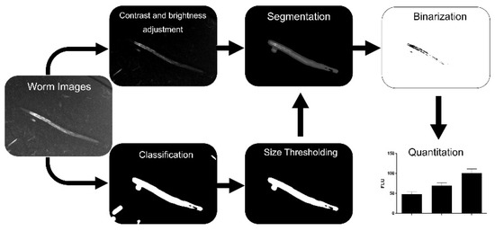
Figure 1.
Workflow of the image processing approach. After fluorescence image acquisition, machine learning classification is performed followed by size thresholding to eliminate false positive areas and manual quality control. Each resulting mask is multiplied with its respective contrast- and brightness-adjusted image. Fluorescent areas are quantified in the segmented images after binarization.
2. Materials and Methods
This section describes our approach to sample preparation, image acquisition, and image processing including classification, segmentation, and quantitation. An overview of the method is shown in Figure 1. Supplementary Material S1 offers a detailed step-by-step instruction of the presented approach. The source code, written in the imageJ macro language, a scripting language built into imageJ, can be found in Supplementary Material S2. The plugin used for image enhancement “Adjust contrast and brightness” is provided with Supplementary Material S3.
2.1. Nile Red Assay
For Nile red assay, the C. elegans mutant strain SS104 with genotype glp-4(bn2) and E. coli OP50 were used. The mutant strain was selected because it shows an elevated fat mass and sterility at the restrictive temperature of 25 °C [35]. Both organisms were obtained from the Caenorhabditis Genetics Center (University of Minnesota). Details of the miniaturized Nile red assay in C. elegans including the composition of all media and reagents have been published recently [21]. Briefly, hermaphrodite animals were maintained on nematode growth medium (NGM) agar plates seeded with 20 µg of OP50 at 16 °C as described by Stiernagle [36]. A synchronized culture was obtained by a bleaching technique, described by Porta-de-la-Riva and coworkers [37]. The synchronized nematodes were grown on fresh agar plates for 12 h at 16 °C, then switched to 25 °C and maintained until they reached the L4 stage. Up to 10 worms were put into each well of a 96-well plate in S-medium containing 10 mg/mL washed and air dried OP50 bacteria and 100 nM Nile red. Vehicle control and test samples were added to reach a final concentration of 1% dimethylsulfoxide (DMSO). Worms were kept under light exclusion at 25 °C for 4 days. Worms were paralyzed with NaN3 prior to imaging using a Zeiss Axio Observer Z1 inverted fluorescence microscope equipped with a rhodamine filter (filter set 20) and an Axio Cam MRm camera system. The numerical aperture of the 5x objective was 0.55. Every worm was imaged using the same settings and same sub-saturating exposure times. Images were saved in tiff-RGB format.
2.2. Data Sets
The images originate from four different experiments in 96-well plates, performed over four consecutive weeks. Each experiment corresponds to one 96-well plate with worms treated by 9 different plant extracts covering the constituents of different lipophilicity and scaffold classes. The image stacks of three experiments were used as external test sets (ETS1-3); the fourth image stack was split into three stacks used to select suitable attribute subsets (TS1-3). Tangling and touching worms in the images were manually excluded from evaluation. Image sets can be found in Supplementary Material Figure S2.
2.3. Image Enhancement
For the correction of defects and enhancement, we developed a plugin for imageJ (Supplementary Material S3) that enables the user to adjust contrast and brightness to the mean and standard deviation (SD) that can be individually set according to a region of interest, a reference image, or predefined numeric values. This step results in a normalized version of the original image, which is calculated using a linear transfer curve (y) as follows:
y = k·x + d
k = (SDset/SDcurrent)
d = meanset − k·meancurrent
The subscript “set” refers to the mean or SD to which the mean or SD of the “current” image is adjusted. Please note that this plugin is integrated as a function, “adjustCB,” in the macro “Find fluorescence in C. elegans” (Supplementary Material S2).
2.4. Training of Classifier
Using FIJI software [38] on a HP tower desktop, 20 images belonging to the training set were converted from RGB- to 8-bit gray level format. Images were scaled to a width of 694 and a height of 520 pixels. In the segmentation settings of the “Trainable Weka Segmentation,” class 1 was defined as “worm” and class 2 as “background.” The option “balance classes” was selected and the “Result overlay opacity” was set to 33. The J48 classifier was selected and the following different training attributes were tested on their applicability for the classification process: Gaussian blur, Hessian, Membrane projections, Mean, Maximum, Anisotropic diffusion, Lipschitz, Gabor, Laplacian, Entropy, Sobel filter, Difference of Gaussians, Variance, Minimum, Median, Bilateral, Kuwahara, Derivatives, Structure, Neighbors. Depending on the filter and where applicable the values of sigma were defined as 1–16 or 16–32, respectively. Areas belonging to the worm were added to the class “worm” with the freehand selection tool as well as areas of the background to the class “background.”
2.5. Selection of Algorithm and Attributes
The selection of the classification algorithm as well as the attribute selection was done with the WEKA software 3.8.3 package [39]. The package provides a collection of machine learning algorithms for data mining tasks. In this study, all algorithms were trained after varying the default settings of WEKA with the given values. The following algorithms were compared using 10-fold cross validation according to their Matthews correlation coefficient (MCC) and the time to build a classifier (Random Tree, J48, LMT tree, Decision stump, Hoeffding tree, Random Forest, REPTree, SMO, Naive Bayes, PART). After selecting an algorithm, classifiers based on 8 different subsets of attributes were trained in the way described in the previous subsection. Instead of selecting all attributes that could be selected for training, the selection was reduced to Entropy, Variance, Hessian, and Laplacian. The combination of those filter subsets with the respective range of sigma and the number of attributes as well as the number of instances are shown in Table 1.

Table 1.
Ranking of attributes using the InfoGainAttributeEvaluation in the WEKA software.
2.6. Evaluation of Attributes on Test Set
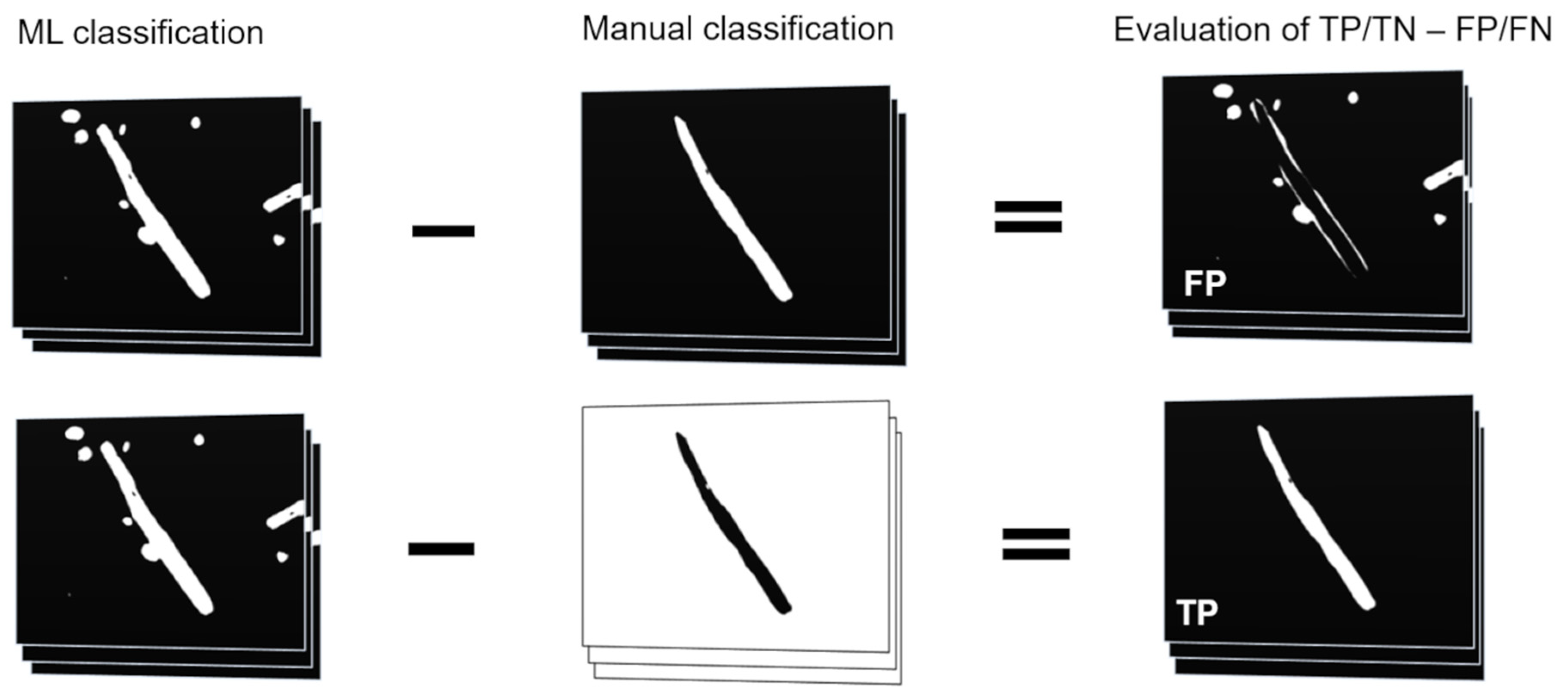
The classifiers that have been trained with the attribute subsets were applied to an external test set of 199 images (ETS1) and compared to the results of manual segmentation of the same test set. All classification results were binarized into two classes: worm and background. Quantitation was performed using the Analyze Particles function. For graphical evaluation of the false positive (FP) area, the manual classification image was subtracted from the machine learning classification result. For the quantitation of the true positive (TP) area, the manual classification result was inverted and subtracted from the machine learning classification. This process is illustrated in Figure 2. The condition positive (P) areas were considered as the quantitation results from the manual process and the background of those images is seen as the condition negative (N) area. True negative (TN) and false negative (FN) true positive rate (TPR), true negative (TNR), accuracy (ACC), MCC, precision (PPV), and F1 value (F1) were calculated as follows:
TN = N − FP, FN = P − TP
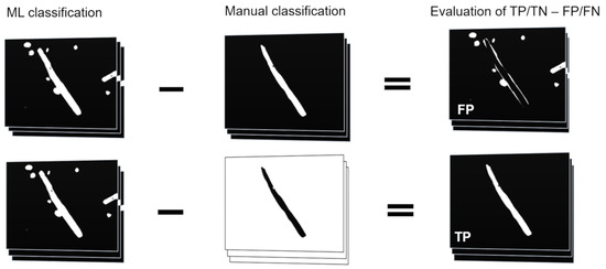
Figure 2.
Calculation of FP and TP areas. Manual classification results were subtracted from machine-learning classification results and the areas were measured to obtain FP and TP values. In case of TP the manual classification results had to be inverted prior to subtraction.
2.7. Evaluation of Size-Thresholding
The classification result of the classifier with subset 1 was edited in FIJI based on the results of the Analyze Particles function. The mean size of single worms was determined by visual inspection, measuring the size of 20 worms with a result of 6283 (±1243) pixels. Various size-thresholds (3000, 3500, 4000, 4500, and 5000 pixels) were validated to differentiate between worm and non-worm areas by comparison of size-thresholded machine learning results to those of manual segmentation. Calculations were performed as described in Evaluation of Attributes on test sets.
2.8. Binarization
Segmented and size-thresholded images were set to “Default dark” and multiplied with the original images using the Image Calculator function. Instead of choosing a general value for transforming the 8-bit grayscale into a binary image using SetThreshold function, the threshold was individually set for each experiment so that 0.3–0.4% of the brightest pixels of the vehicle control group worms contained the value white (1). Once the threshold was determined, it was applied to all images belonging to the same experiment. Afterwards the pixels containing the value white (1) were measured by the “Analyze Particles” function. The measured value of each worm corresponds to the fluorescence of the worm.
2.9. Experimental Validation, Nile Red Assay
The applicability of the presented method was outlined using positive controls fluoxetine and 5-aminoimidazole-4-carboxamide ribonucleotide (AICAR) as an application example in [21]. Fluoxetine (F-132) and AICAR (A9978) were obtained from Sigma Aldrich with a purity of ≥98%. Each treatment and concentration was tested in 6-well replicates with up to 10 worms per well. The mean worm fluorescence (measured pixels with a value of 1) of each treatment cohort was calculated. The experiments were performed three times independently and the mean fluorescence was presented ± SD. GraphPad Prism 4.03 software was used for statistical analyses; statistical significance of the differences between vehicle and treatment groups were tested by ANOVA (analysis of variance) with Bonferroni post-test.
2.10. Experimental Validation, Triacyl Glyceride Assay
Two cohorts of approximately 1400 L4 worms at a density of 200 worms/mL in S medium supplemented with 10 mg/mL OP50 as a food source were incubated at 25 °C under agitation. Depending on the sample vehicle control 1% DMSO, 100 µM fluoxetine, or 100 µM AICAR was added. After four days of treatment, worms were cleared of bacteria and media by washing with ddH2O and multiple centrifugation/decantation steps. The bacteria-free worm pellets were lyophilized, taken up in 100 µL 5% Nonidet and then lysed using a bioruptor plus sonication system (Diagenode, Liège, Belgium) at 4 °C and in 30 high intensity 30 s on/off cycles. The lysate was heated to 95 °C for 5 min, and after cooling, 50 µL of the lysates were set aside for the TAG assay. The other 50 µL were supplemented with 100 µL of RIPA lysis buffer and lysed again in 100 high intensity cycles, centrifuged and the supernatant used for bicinchoninic acid (BCA) assay. The TAG assay was performed using triglyceride quantification kit from Sigma-Aldrich (Sigma-Aldrich Handels Gmbh, Wien, Austria) (MAK-266) according to the manufacturer’s instructions. A six step concentration series of trioleate standard in assay buffer in two technical replicates, and a ten-fold diluted sample lysates in four replicates (and two further technical replicates for background control) were pipetted into a black 96-well plate and incubated with lipase at room temperature. No lipase was added to the background control wells. After 20 min, a TAG probe and enzyme mix were added. After an incubation time of 60 min under light exclusion, fluorescence intensity was measured with a Tecan Sparks (Tecan, Grödig, Austria), excitation wavelength 535 nm (bandwidth 25 nm), emission wavelength 590 nm (bandwidth 20 nm). Protein quantification was performed using the BCA assay kit (BCA1) from Sigma-Aldrich according to the manufacturer’s instructions for 96-well plates. Sample lysates and a dilution series of BSA protein standard were added in duplicates to the wells of a clear 96-well plate. Following this, BCA working reagent, consisting of copper (II) sulfate pentahydrate and BCA solution, was added and the plate was incubated for 30 min at 37 °C. Afterwards, the absorbance was measured with a Tecan Sparks (Tecan, Grödig, Austria) at 562 nm.
3. Results
3.1. Segmentation/Selection of the Machine Learning Algorithm and Attribute Subset
For the selection of the most-suited machine learning algorithm, twelve classifiers were compared according to their MCC and time to build the ten-fold cross correlation model using default parameters in the software. For this purpose, a dataset of 20 labeled images based on all 141 attributes available in the Trainable WEKA Segmentation plug-in was evaluated (Supplementary Material Figure S1). Because the MCC value differed only slightly between all trees, it was decided to focus on those trees that perform pruning (Random, J48, and LMT), meaning that parts with little impact on classifying instances are removed. The resulting smaller tree that does not perfectly classify every pixel of the training set is less prone to overfitting. The J48 tree was selected for further evaluation as it is based on the C4.5 algorithm listed as one of the top ten algorithms in data mining [40].
For selecting the best-suited attributes, the classifying power of each attribute was evaluated by measuring the information gain with respect to a class, using the WEKA InfoGainAttributeEval algorithm. The algorithm measures how each feature contributes to decreasing the overall entropy. Thereby, the value of an attribute is calculated as follows:
where H(Class) is the marginal entropy of the class and H(Class|Attribute) is the conditional entropy of the class with respect to the attribute. The InfoGainAttributeEval algorithm was chosen for attribute evaluation, since the previously selected ML algorithm J48 is based on the same principle of evaluating the worth of attributes for the classification process. Therefore, the InfoGainAttributeEval algorithm can be used to rank the attributes that are of value for the J48 algorithm. Based on the results in the ranking, attributes can be removed that would be cut off by the J48 pruning tree regardless. In this way, the process can be sped up by eliminating redundant attributes prior to the ML classification process. The resulting ranking, with the top-scoring 50 attributes, is shown in Table 1.
InfoGain(Class,Attribute) = H(Class) − H(Class|Attribute)
Classifiers which are based on different subsets of attributes were compared according to their performance on three image tests sets (TS1: 67 images; TS2: 66 images; TS3: 66 images). The test sets were compared to manually classified images. The evaluation started with a test of a classifier considering the full range of image attributes for decision making. Each following classifier was simplified, whereby the subset with the lowest contribution to classifying power, calculated by the InfoGainAttributeEval algorithm, was removed, resulting in the eight classifiers shown in Figure 3. Filters used in the subset selection include entropy (ENT), variance (VAR), Hessian (HES), and Laplacian (LAP).
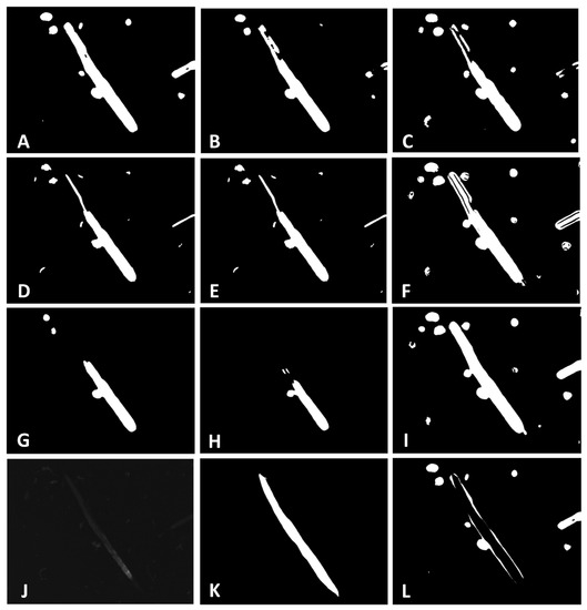
Figure 3.
(A–H) Classification results of classifiers with different subsets; (I) all available filters; (J) original worm image; (K) mask created by manual classification; (L) false positive (FP) areas after classification based on Subset 1.
All classification results were binarized into two classes: worm (=white (1)) and background (=black (0)). Quantitation was performed in FIJI using the Analyze Particles function and the following values were calculated: TP, FP, FN, TN, TPR, TNR, ACC, and the MCC. It could be observed that Subset 1, which uses 22 attributes based on entropy with a sigma range of 1-16 for decision making, led to a classifier that showed the highest ACC (94.56%), sensitivity (73.48%), specificity (96.63%), and MCC (67.99%), resulting in the best performance for the three test sets TS1-3 (Table 2, Figure 4). Performance is hereby calculated as mean of ACC, TPR, TNR, and MCC.
Table 2.
Evaluation of the performance of different attribute subsets on test sets (TS1-TS3). Performance is calculated as mean of ACC, TPR, TNR and MCC.
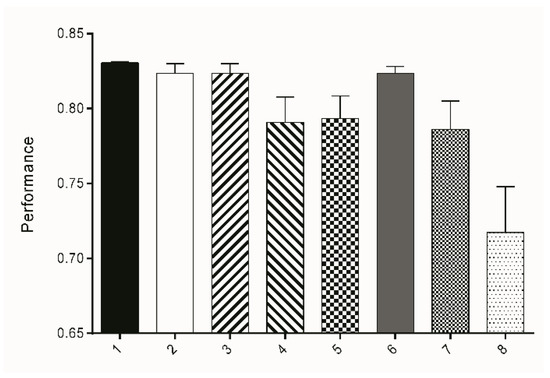
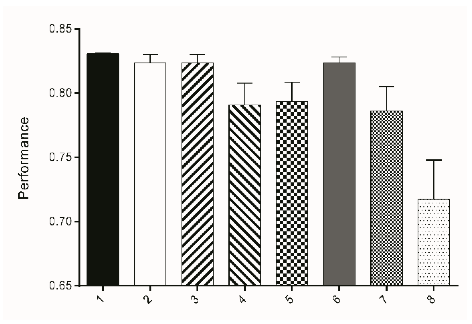
Figure 4.
Bars represent the mean performance (±SD) of attribute subsets 1–8 derived from three test sets TS1-3. The performance was calculated as the mean value of TPR, TNR, ACC, and MCC.
3.2. Segmentation/Size-Thresholding Settings
As can be seen in Figure 3, the largest classified areas of the images belong to the worm, whereas unattached areas are considerably smaller and belong to FP. To select the best settings for the size of the areas that should be removed from the classification result (termed size-thresholding), a histogram showing the areas of test sets TS1-3 was created (Figure 5) to visually demonstrate a valid size cut-off between FP areas and the worm. The histogram shows bell-shaped distributions; the most left one in Figure 5 belongs to objects below 4000 pixels consisting only of objects that do not belong to nematodes as verified by visual inspection, while the remaining objects are considered worms. The minimum between these two distributions is indicated in Figure 5 by a red line. This observation was evaluated after applying five different cut-offs ranging from 3000 to 5000 pixels. The performance is calculated as the mean value of the resulting TPR, TNR, ACC, and MCC, showing the highest performance of 0.8478 at the cut-off of 4000 pixels. Using this setting for size-thresholding additionally to the classification process, the MCC could be improved from 68.0% to 73.2%, while the ACC, sensitivity, and specificity could be increased by 1% each.
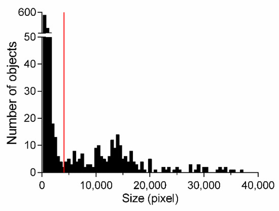
Figure 5.
Histogram of all classified areas measured in test sets TS1-3 based on attribute subset 1. Bars represent the number of objects with a certain area (pixel); the red bar indicates the minimum between two distributions.
3.3. Validation
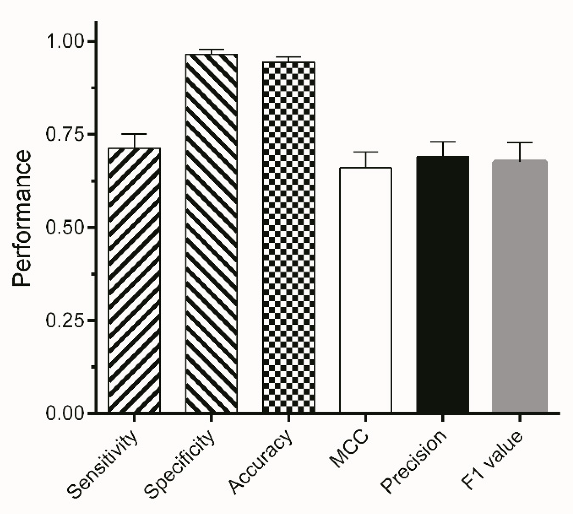
The final segmentation method is based on the J48 algorithm using the entropy filter with a range of sigma from 1 to 16 and subsequently excluding areas with a size smaller than 4000 pixels from the binary image. Results of the classification process—available as binary masks—were multiplied with the original images. For validation, three external test sets (ETS1-3) were used consisting of 117, 121, and 137 images, respectively. The segmentation method shows a high specificity and ACC of more than 90% for all three external test sets (Figure 6). This indicates that background areas of the image were correctly assigned giving a high TNR. A total of 67–75% of areas classified as worms were correctly assigned, which is eminently proficient giving the fact that manual segmentation is subject to inter-operator variations of approximately 20% [41,42,43]. Moreover, the automated segmentation reduces the time of user interaction by 75%.
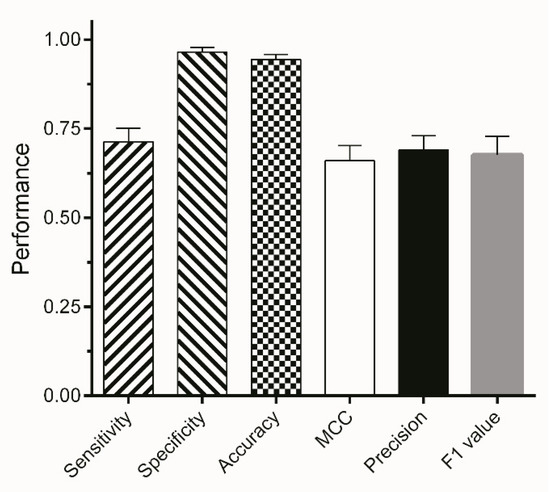
Figure 6.
Mean performance metrics of segmentation on three different external test sets. Bars represent the mean value of TPR, TNR, ACC, MCC, PPV, and F1 of ETS1-3 ± SD.
3.4. Binarization
The resulting segmented images were binarized for fluorescence quantitation. Setting a fixed value for the global thresholding binarization led to high SD in the results. Setting the value for each experiment individually, so that 0.3–0.4% of the brightest pixels of the vehicle control group worms contained the value white, resulted in a high reproducibility of results.
In order to evaluate the performance of the complete image processing workflow, the number of measured pixels after FP results were manually removed was compared to the results without manual quality control. Application of the whole image processing method led to an ACC of 0.998 (±0.001) and an MCC of 0.833 (±0.034), as shown in Table 3.
Table 3.
Mean performance of machine learning classification combined with binarization obtained for external test sets ETS1-3.
3.5. Experimental Validation
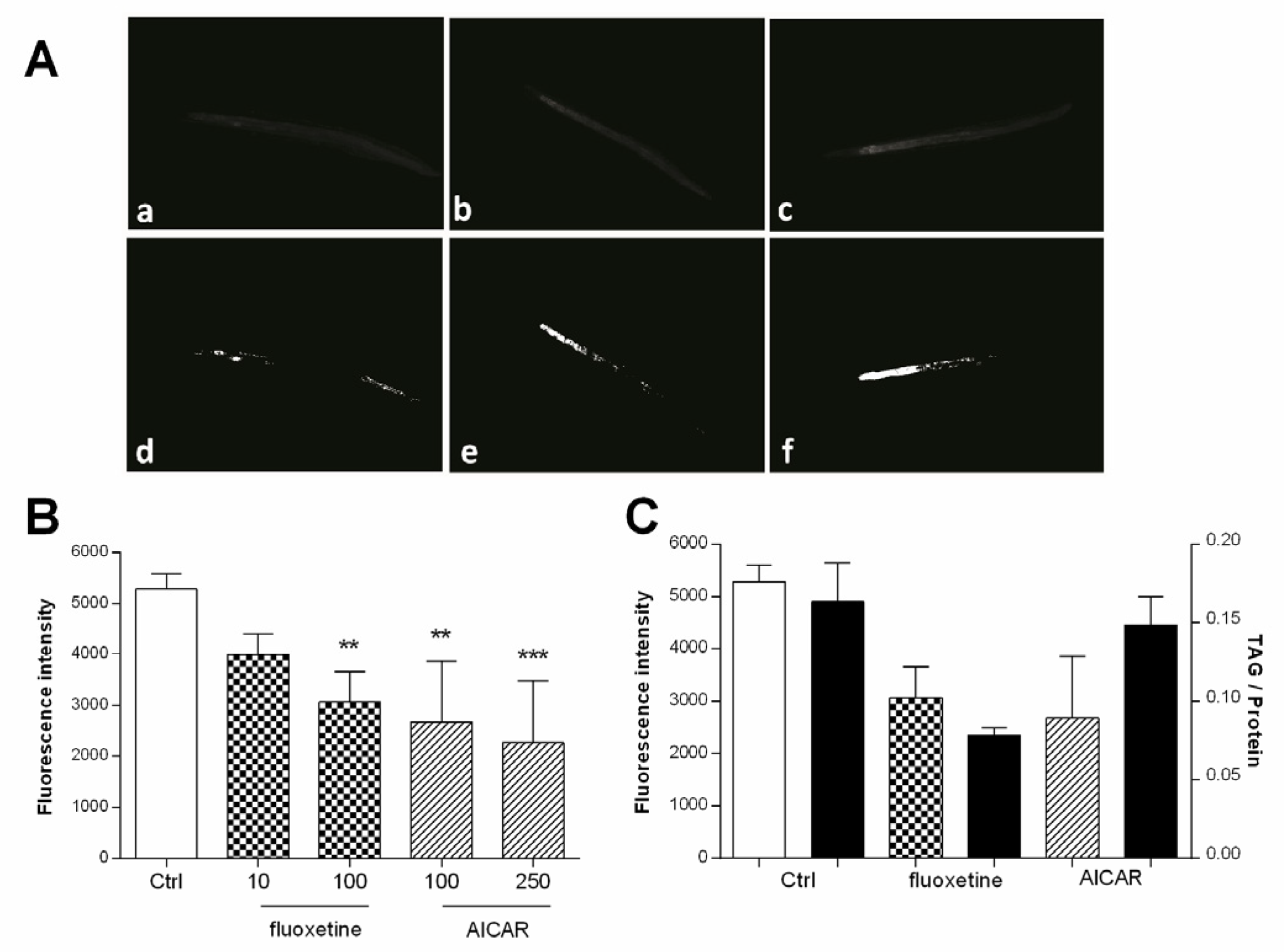
The applicability of the method presented herein, summarized in Figure 1, has been demonstrated before [21]. The results are briefly outlined here using the drugs fluoxetine and AICAR. AICAR and fluoxetine were previously reported to reduce Nile red fluorescence in C. elegans [17], and were therefore selected as positive controls for the validation of our image processing method. The two agents were tested in three independent experiments and the images were evaluated using the presented workflow. The mean fluorescence of three experiments is shown in Figure 7B. Fluoxetine significantly reduced fluorescence to 58.0% (±5.9) at 100 µM and 75.6% (±4.1) at 10 µM, while AICAR significantly reduced fluorescence to 42.9% (±12.4) at 250 µM and 50.6% (±11.9) at 100 µM, compared to vehicle-treated worms. Biochemical TAG quantification showed a similar reduction of TAG with a TAG/protein ratio of 47.8% after treatment with 100 µM fluoxetine and 90.5% with 100 µM AICAR (Figure 7C).
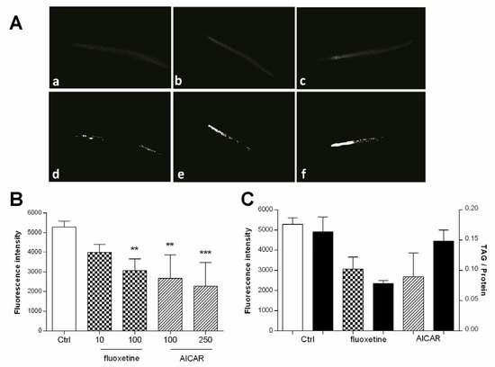
Figure 7.
(A) Representative images of worms treated with (a) fluoxetine (100 µM), (b) fluoxetine (10 µM), (c) vehicle control (1% DMSO), and their corresponding areas measured after binarization (d–f) (B) Bar charts represent the mean Nile red fluorescence of worms from three independent experiments (± SD). Worms were treated with Ctrl (vehicle control, 1% DMSO), fluoxetine (10 µM and 100 µM), and AICAR (100 µM and 250 µM). The significance was assessed by one-way ANOVA and Bonferroni post-test (** p < 0.01, *** p < 0.001). (C) White bars represent either Nile red fluorescence (n = 3; ±SD) compared to black bars representing extracted and biochemically quantified TAG content of worms relative to protein content (n = 2; ±SD). Worms were treated with Ctrl (vehicle control, 1% DMSO), fluoxetine (100 µM), and AICAR (100 µM).
4. Discussion
Entropy attributes—The concept of entropy is well established in bioimage segmentation and is also the most important attribute in the presented classification process. One reason for the superiority of entropy over geometric attributes, e.g., mean and variance, or structure-based filters, for our application can be explained by the high number of transitions of brightness values in the stained worm intestine compared to the background. Background fluorescence transitions, e.g., from large bacterial clusters and remains from worm molting show, similar to worm fluorescence, a high amount of brightness transitions, and are thus occasionally identified as worms by segmentation. However, these areas are usually small and are removed by size thresholding. Other fluorescence signals, e.g., from bacteria, are too weak and are removed upon binarization. Thus, the sensitivity increases from 73.0% for correct assignment of worms on images to 99.7% for correct assignment of worm fluorescence.
Reproducibility—The reproducibility of treatment effects (Figure 7B) was improved by setting thresholds for global binarization corresponding to the brightest pixels of the vehicle control group worms. Fixed global thresholding values have been shown to be insufficient due to an unpreventable variance in the staining of biological systems, such as worms and bacteria. Exemplary sources of variance between experiments are different quality foods, slightly diverse worm populations, and the handling of Nile red, which is known to bind to polypropylene [44], among other substances [45]. It is speculated that most of these factors affect control worms and treated worms in the same way. Setting the value for each experiment individually so that 0.3–0.4% of pixels were contained the value white resulted in a high reproducibility of results. Additionally, Mori and coworkers [16] set their staining intensities relative to the staining intensities of control worms.
Segmentation—Compared to established methods, the accuracy of the presented worm segmentation is low. The mean F1 value of our segmentation is 0.67. The method of Fudickar and coworkers [29] achieved an F1 value of 0.93. The worm segmentation also results in inaccurate representation of the worm size. This makes certain measurements on images dubious, such as the measurement of worm size and fluorescence density (fluorescence relative to worm areas). Hence, it is difficult to compare our results with studies that quantify fluorescence densities [18,32]. Moreover, the fluorescence of very small worms cannot be compared to very large worms. Thus, agents that inhibit a normal worm development have to be excluded from analysis. The relevance of such nematotoxic compounds for metabolic disease drug discovery is generally questionable. It is further not possible to untangle worms in a way as described by Wählby and coworkers [30]. This limits the number of worms per well to prevent them from becoming entangled.
Fluorescence quantitation—Besides the different techniques for segmenting worms, widely varying methods for quantifying fluorescence have been reported in the literature—e.g., Lemieux and coworkers [17] quantified the total integrated fluorescence intensity of only the two most anterior cells and corrected for background fluorescence with a Gaussian segmentation mask; others used the total staining intensity relative to the area of worm regions [15,16,18]. Jia and coworkers [46] measured fluorescence as the area of lipid droplets in a circle posterior to the second bulb of the pharynx. Next to global thresholding for binarizations, there are also studies that used auto thresholding, e.g., the Triangle Threshold [47]. We compared the performance of different binarization methods for reproducibility between independent experiments and the agreement with the results of the biochemical TAG assay. Setting the worm regions relative to the area of segmented worms led to a deterioration of results. This was attributed to the limited performance of the segmentation on very low-fluorescent worms. Because of the limited staining and, thus, the low pixel entropies in the head and tail of the worms, these areas are sometimes segmented as background (Figure 3). However, these segmentation errors have no effect on our binarization method. As shown in Table 3, there is only a minor difference between the quantification of manually segmented and automatically segmented worms using global threshold binarization set to the mean of control.
Positive controls—The first positive control, fluoxetine, is approved as an antidepressant by the FDA and EMA and has shown anti-obesity effects in humans, proposed to be due to an increased serotonergic activity in the brain [48,49,50]. The second positive control, AICAR, is an investigational drug which reduces neutral lipid content in adipocytes and showed anti-obesity effects in a mouse model [51]. Fluoxetine and AICAR have also been reported to inhibit fat accumulation in C. elegans by independent mechanisms [17,52]. Fluoxetine inhibits fat accumulation through increased neural serotoninergic signaling leading to an increased beta-oxidation [52]. Recently, a study demonstrated an increased fat accumulation in C. elegans in response to fluoxetine treatment [53], but different conditions were used. AICAR inhibits fat accumulation through the activation of the cellular energy hub AMP-activated protein kinase (AMPK) [17]. The inhibition of fat accumulation by the two compounds was also confirmed in our experiments. In this regard, the results of the TAG assay were comparable to the results of our Nile red assay quantified by the image processing process presented (Figure 7C). Thus, it can be concluded that the image processing workflow is suitable for the quantitation of Nile red stained lipids in C. elegans. However, it is important to note that the absolute quantitation achieved from Nile red staining and biochemical lipid determination sometimes (as in the case of AICAR) does not match perfectly. This has also been reported previously [18].
5. Conclusions
Using supervised learning and the addition of a size-threshold filter, we were able to train a proficient classifier for the segmentation of worms on fluorescence images. Setting the binarization according to control group images made the quantitation particularly robust and delivers results with appropriate reproducibility. Since there is a lack of well described routines for these image processing methods, we wrote a script in the macro language of imageJ and share it in Supplementary Material S2. The presented workflow as highlighted in Figure 1 offers: (1) reliable results with a high accuracy (2) decreased time of user-interaction for image segmentation, and (3) a user-friendly view of the segmented image enabling accurate quality control.
The script can be quickly established and adapted to the requirements of different fluorescence-staining assays. In this work we presented its performance on vital Nile red stained worms. However, an application to images of worms stained with other fluorescence dyes is possible. The protocol therefore offers steps for individual specifications of size thresholding, contrast and brightness adjustment, and settings for binarization, including the manual control of classification results.
It is important to add that the Nile red assay used in this study is not able to quantify TAG from storage droplets [15], and is rather an indirect measure [4,54]. However, the assay, as well as the image processing workflow, is easy to use, easy to implement, fast, and sensitive. It can facilitate the prioritization of agents, e.g., from natural sources [21], for further analysis. Most importantly, the image processing workflow facilitates segmentation for sufficient fluorescence quantitation directly from the fluorescence images, eliminating the need to capture brightfield images.
Supplementary Materials
The following are available online at https://www.mdpi.com/article/10.3390/app112311420/s1, S1: Step-by-step instruction, S2: Code “Find fluorescence in C. elegans”, S3: Code “ADJUST CB”, Figure S1: Validation of machine learning algorithms, Figure S2: Biochemical TAG quantification.
Author Contributions
Conceptualization, B.K. and J.M.R.; methodology, D.P.; software, T.L. and D.P.; validation, T.L., D.P. and B.K.; formal analysis, T.L. and D.P.; investigation, T.L. and B.K.; resources, J.M.R.; data curation, T.L.; writing—original draft preparation, T.L.; writing—review and editing, J.M.R., D.P. and B.K; visualization, T.L. and B.K.; supervision, J.M.R.; project administration, B.K.; funding acquisition, J.M.R. All authors have read and agreed to the published version of the manuscript.
Funding
This research received no external funding.
Institutional Review Board Statement
Not applicable.
Informed Consent Statement
Not applicable.
Data Availability Statement
The data presented in this study are available on request from the corresponding author.
Acknowledgments
The authors want to thank Martina Redl and Ruzica Colic for the excellent technical assistance and proofreading of this work. We thank the CGC, which is funded by NIH Office of Research Infrastructure Programs (P40 OD010440), for providing OP50 bacteria and SS104 worms. (Open Access Funding by the University of Vienna).
Conflicts of Interest
The authors declare no conflict of interest.
References
- Hulme, S.E.; Whitesides, G.M. Chemistry and the worm: Caenorhabditis elegans as a platform for integrating chemical and biological research. Angew. Chem. Int. Ed. Engl. 2011, 50, 4774–4807. [Google Scholar] [CrossRef] [Green Version]
- Schulenburg, H.; Félix, M.-A. The Natural Biotic Environment of Caenorhabditis elegans. Genetics 2017, 206, 55–86. [Google Scholar] [CrossRef] [PubMed] [Green Version]
- O’Reilly, L.P.; Luke, C.J.; Perlmutter, D.H.; Silverman, G.A.; Pak, S.C. C. elegans in high-throughput drug discovery. Adv. Drug Deliv. Rev. 2014, 69–70, 247–253. [Google Scholar] [CrossRef] [Green Version]
- Lemieux, G.A.; Ashrafi, K. Insights and challenges in using C. elegans for investigation of fat metabolism. Crit. Rev. Biochem. Mol. Biol. 2015, 50, 69–84. [Google Scholar] [CrossRef] [PubMed]
- Jones, K.T.; Ashrafi, K. Caenorhabditis elegans as an emerging model for studying the basic biology of obesity. Dis. Model. Mech. 2009, 2, 224–229. [Google Scholar] [CrossRef] [PubMed] [Green Version]
- Shen, P.; Yue, Y.; Park, Y. A living model for obesity and aging research: Caenorhabditis elegans. Crit. Rev. Food Sci. Nutr. 2018, 58, 741–754. [Google Scholar] [CrossRef]
- Soukas, A.A.; Kane, E.A.; Carr, C.E.; Melo, J.A.; Ruvkun, G. Rictor/TORC2 regulates fat metabolism, feeding, growth, and life span in Caenorhabditis elegans. Genes Dev. 2009, 23, 496–511. [Google Scholar] [CrossRef] [PubMed] [Green Version]
- Ezcurra, M.; Benedetto, A.; Sornda, T.; Gilliat, A.F.; Au, C.; Zhang, Q.; van Schelt, S.; Petrache, A.L.; Wang, H.; de la Guardia, Y.; et al. C. elegans eats its own intestine to make yolk leading to multiple senescent pathologies. Curr. Biol. 2018, 28, 2544–2556. [Google Scholar] [CrossRef]
- Salzer, L.; Witting, M. Quo vadis Caenorhabditis elegans metabolomics—A review of current methods and applications to explore metabolism in the nematode. Metabolites 2021, 11, 284. [Google Scholar] [CrossRef] [PubMed]
- Grant, B.; Hirsh, D. Receptor-mediated endocytosis in the Caenorhabditis elegans oocyte. Mol. Biol. Cell 1999, 10, 4311–4326. [Google Scholar] [CrossRef] [PubMed] [Green Version]
- Zhang, P.; Na, H.; Liu, Z.; Zhang, S.; Xue, P.; Chen, Y.; Pu, J.; Peng, G.; Huang, X.; Yang, F. Proteomic study and marker protein identification of Caenorhabditis elegans lipid droplets. Mol. Cell. Proteom. 2012, 11, 317–328. [Google Scholar] [CrossRef] [PubMed] [Green Version]
- Chen, W.W.; Lemieux, G.A.; Camp, C.H., Jr.; Chang, T.C.; Ashrafi, K.; Cicerone, M.T. Spectroscopic coherent Raman imaging of Caenorhabditis elegans reveals lipid particle diversity. Nat. Chem. Biol. 2020, 16, 1087–1095. [Google Scholar] [CrossRef] [PubMed]
- Chen, W.W.; Yi, Y.H.; Chien, C.H.; Hsiung, K.C.; Ma, T.H.; Lin, Y.C.; Lo, S.J.; Chang, T.C. Specific polyunsaturated fatty acids modulate lipid delivery and oocyte development in C. elegans revealed by molecular-selective label-free imaging. Sci. Rep. 2016, 6, 32021. [Google Scholar] [CrossRef] [PubMed] [Green Version]
- Hellerer, T.; Axäng, C.; Brackmann, C.; Hillertz, P.; Pilon, M.; Enejder, A. Monitoring of lipid storage in Caenorhabditis elegans using coherent anti-Stokes Raman scattering (CARS) microscopy. Proc. Natl. Acad. Sci. USA 2007, 104, 14658–14663. [Google Scholar] [CrossRef] [Green Version]
- O’Rourke, E.J.; Soukas, A.A.; Carr, C.E.; Ruvkun, G. C. elegans major fats are stored in vesicles distinct from lysosome-related organelles. Cell Metab. 2009, 10, 430–435. [Google Scholar] [CrossRef] [PubMed] [Green Version]
- Mori, A.; Holdorf, A.D.; Walhout, A.J.M. Many transcription factors contribute to C. elegans growth and fat storage. Genes Cells 2017, 22, 770–784. [Google Scholar] [CrossRef] [Green Version]
- Lemieux, G.A.; Liu, J.; Mayer, N.; Bainton, R.J.; Ashrafi, K.; Werb, Z. A whole-organism screen identifies new regulators of fat storage. Nat. Chem. Biol. 2011, 7, 206–213. [Google Scholar] [CrossRef] [Green Version]
- Pino, E.C.; Webster, C.M.; Carr, C.E.; Soukas, A.A. Biochemical and high throughput microscopic assessment of fat mass in Caenorhabditis elegans. J. Vis. Exp. 2013, 30, e50180. [Google Scholar] [CrossRef] [PubMed] [Green Version]
- Pang, S.; Lynn, D.A.; Lo, J.Y.; Paek, J.; Curran, S.P. SKN-1 and Nrf2 couples proline catabolism with lipid metabolism during nutrient deprivation. Nat. Commun. 2014, 5, 5048. [Google Scholar] [CrossRef] [Green Version]
- Huang, W.M.; Li, Z.Y.; Xu, Y.J.; Wang, W.; Zhou, M.G.; Zhang, P.; Liu, P.S.; Xu, T.; Wu, Z.X. PKG and NHR-49 signalling co-ordinately regulate short-term fasting-induced lysosomal lipid accumulation in C. elegans. Biochem. J. 2014, 461, 509–520. [Google Scholar] [CrossRef] [PubMed]
- Zwirchmayr, J.; Kirchweger, B.; Lehner, T.; Tahir, A.; Pretsch, D.; Rollinger, J.M. A robust and miniaturized screening platform to study natural products affecting metabolism and survival in Caenorhabditis elegans. Sci. Rep. 2020, 10, 12323. [Google Scholar] [CrossRef]
- Rizwan, I.; Haque, I.; Neubert, J. Deep learning approaches to biomedical image segmentation. Inform. Med. Unlocked 2020, 18, 100297. [Google Scholar] [CrossRef]
- Husson, S.J.; Costa, W.S.; Schmitt, C.; Gottschalk, A. Keeping Track of Worm Trackers; WormBook: Pasadena, CA, USA, 2013; pp. 1–17. [Google Scholar]
- Kabra, M.; Conery, A.; O’Rourke, E.; Xie, X.; Ljosa, V.; Jones, T.; Ausubel, F.; Ruvkun, G.; Carpenter, A.; Freund, Y. Towards automated high-throughput screening of C. elegans on agar. arXiv 2010, arXiv:1003.4287. [Google Scholar]
- Hernando-Rodríguez, B.; Erinjeri, A.P.; Rodríguez-Palero, M.J.; Millar, V.; González-Hernández, S.; Olmedo, M.; Schulze, B.; Baumeister, R.; Muñoz, M.J.; Askjaer, P.; et al. Combined flow cytometry and high-throughput image analysis for the study of essential genes in Caenorhabditis elegans. BMC Biol. 2018, 16, 36. [Google Scholar] [CrossRef] [PubMed]
- Hakim, A.; Mor, Y.; Toker, I.A.; Levine, A.; Neuhof, M.; Markovitz, Y.; Rechavi, O. WorMachine: Machine learning-based phenotypic analysis tool for worms. BMC Biol. 2018, 16, 8. [Google Scholar] [CrossRef] [PubMed] [Green Version]
- Moore, B.T.; Jordan, J.M.; Baugh, L.R. WormSizer: High-throughput Analysis of Nematode Size and Shape. PLoS ONE 2013, 8, e57142. [Google Scholar]
- Bornhorst, J.; Nustede, E.J.; Fudickar, S. Mass Surveilance of C. elegans-Smartphone-Based DIY Microscope and Machine-Learning-Based Approach for Worm Detection. Sensors 2019, 19, 1468. [Google Scholar] [CrossRef] [Green Version]
- Fudickar, S.; Nustede, E.J.; Dreyer, E.; Bornhorst, J. Mask R-CNN Based C. Elegans Detection with a DIY Microscope. Biosensors 2021, 11, 257. [Google Scholar] [CrossRef]
- Wählby, C.; Kamentsky, L.; Liu, Z.H.; Riklin-Raviv, T.; Conery, A.L.; O’Rourke, E.J.; Sokolnicki, K.L.; Visvikis, O.; Ljosa, V.; Irazoqui, J.E.; et al. An image analysis toolbox for high-throughput C. elegans assays. Nat. Methods 2012, 9, 714–716. [Google Scholar] [CrossRef] [Green Version]
- Carpenter, A.E.; Jones, T.R.; Lamprecht, M.R.; Clarke, C.; Kang, I.H.; Friman, O.; Guertin, D.A.; Chang, J.H.; Lindquist, R.A.; Moffat, J.; et al. CellProfiler: Image analysis software for identifying and quantifying cell phenotypes. Genome Biol. 2006, 7, R100. [Google Scholar] [CrossRef] [PubMed] [Green Version]
- Escorcia, W.; Ruter, D.L.; Nhan, J.; Curran, S.P. Quantification of Lipid Abundance and Evaluation of Lipid Distribution in Caenorhabditis elegans by Nile Red and Oil Red O Staining. J. Vis. Exp. 2018, 133, 57352. [Google Scholar] [CrossRef] [PubMed]
- Wang, L.; Kong, S.; Pincus, Z.; Fowlkes, C. Celeganser: Automated analysis of nematode morphology and age. In Proceedings of the IEEE/CVF Conference on Computer Vision and Pattern Recognition (CVPR) Workshops, Seattle, WA, USA, 14–19 June 2020; pp. 968–969. [Google Scholar]
- Chen, L.; Strauch, M.; Daub, M.; Jiang, X.; Jansen, M.; Luigs, H.-G.; Schultz-Kuhlmann, S.; Krussel, S.; Merhof, D. A CNN Framework Based on Line Annotations for Detecting Nematodes in Microscopic Images. In Proceedings of the 2020 IEEE 17th International symposium on biomedical imaging (ISBI), Iowa City, IA, USA, 3–7 April 2020; pp. 508–512. [Google Scholar]
- Rastogi, S.; Borgo, B.; Pazdernik, N.; Fox, P.; Mardis, E.R.; Kohara, Y.; Havranek, J.; Schedl, T. Caenorhabditis elegans glp-4 Encodes a Valyl Aminoacyl tRNA Synthetase. G3 2015, 5, 2719–2728. [Google Scholar] [CrossRef] [PubMed] [Green Version]
- Stiernagle, T. Maintenance of C. elegans; Worm Book: Pasadena, CA, USA, 2006; pp. 1–11. [Google Scholar]
- Porta-de-la-Riva, M.; Fontrodona, L.; Villanueva, A.; Cerón, J. Basic Caenorhabditis elegans methods: Synchronization and observation. J. Vis. Exp. 2012, 64, e4019. [Google Scholar] [CrossRef] [PubMed] [Green Version]
- Schindelin, J.; Arganda-Carreras, I.; Frise, E.; Kaynig, V.; Longair, M.; Pietzsch, T.; Preibisch, S.; Rueden, C.; Saalfeld, S.; Schmid, B.; et al. Fiji: An open-source platform for biological-image analysis. Nat. Methods 2012, 9, 676–682. [Google Scholar] [CrossRef] [PubMed] [Green Version]
- Hall, M.; Frank, E.; Holmes, G.; Pfahringer, B.; Reutemann, P.; Witten, I.H. The WEKA data mining software: An update. ACM SIGKDD Explor. Newsl. 2009, 11, 10–18. [Google Scholar] [CrossRef]
- Wu, X.; Kumar, V.; Quinlan, J.R.; Ghosh, J.; Yang, Q.; Motoda, H.; McLachlan, G.J.; Ng, A.; Liu, B.; Yu, P.S.; et al. Top 10 algorithms in data mining. Knowl. Inf. Syst. 2008, 14, 1–37. [Google Scholar] [CrossRef] [Green Version]
- Bechara, B.P.; Leckie, S.K.; Bowman, B.W.; Davies, C.E.; Woods, B.I.; Kanal, E.; Sowa, G.A.; Kang, J.D. Application of a semiautomated contour segmentation tool to identify the intervertebral nucleus pulposus in MR images. Am. J. Neuroradiol. 2010, 31, 1640–1644. [Google Scholar] [CrossRef] [PubMed] [Green Version]
- Millioni, R.; Sbrignadello, S.; Tura, A.; Iori, E.; Murphy, E.; Tessari, P. The inter- and intra-operator variability in manual spot segmentation and its effect on spot quantitation in two-dimensional electrophoresis analysis. Electrophoresis 2010, 31, 1739–1742. [Google Scholar] [CrossRef] [PubMed]
- Shahedi, M.; Cool, D.W.; Romagnoli, C.; Bauman, G.S.; Bastian-Jordan, M.; Gibson, E.; Rodrigues, G.; Ahmad, B.; Lock, M.; Fenster, A.; et al. Spatially varying accuracy and reproducibility of prostate segmentation in magnetic resonance images using manual and semiautomated methods. Med. Phys. 2014, 41, 113503. [Google Scholar] [CrossRef] [PubMed]
- Maes, T.; Jessop, R.; Wellner, N.; Haupt, K.; Mayes, A.G. A rapid-screening approach to detect and quantify microplastics based on fluorescent tagging with Nile Red. Sci. Rep. 2017, 7, 44501. [Google Scholar] [CrossRef] [PubMed] [Green Version]
- Lithgow, G.J.; Driscoll, M.; Phillips, P. A long journey to reproducible results. Nature 2007, 548, 387–388. [Google Scholar] [CrossRef] [Green Version]
- Jia, R.; Zhang, J.; Jia, K. Neuroendocrine regulation of fat metabolism by autophagy gene atg-18 in C. elegans dauer larvae. FEBS Open Bio 2019, 9, 1623–1631. [Google Scholar] [CrossRef] [Green Version]
- Navarro-Herrera, D.; Aranaz, P.; Eder-Azanza, L.; Zabala, M.; Hurtado, C.; Romo-Hualde, A.; Martínez, J.A.; González-Navarro, C.J.; Vizmanos, J.L. Dihomo-gamma-linolenic acid induces fat loss in C. elegans in an omega-3-independent manner by promoting peroxisomal fatty acid β-oxidation. Food Funct. 2018, 9, 1621–1637. [Google Scholar] [CrossRef] [PubMed]
- Gray, D.S.; Fujioka, K.; Devine, W.; Bray, G.A. A randomized double-blind clinical trial of fluoxetine in obese diabetics. Int. J. Obes. Relat. Metab. Disord. 1992, 16 (Suppl. 4), S67–S72. [Google Scholar] [PubMed]
- Goldstein, D.J.; Rampey, A.H., Jr.; Enas, G.G.; Potvin, J.H.; Fludzinski, L.A.; Levine, L.R. Fluoxetine: A randomized clinical trial in the treatment of obesity. Int. J. Obes. Relat. Metab. Disord. 1994, 18, 129–135. [Google Scholar] [PubMed]
- Levine, L.R.; Enas, G.G.; Thompson, W.L.; Byyny, R.L.; Dauer, A.D.; Kirby, R.W.; Kreindler, T.G.; Levy, B.; Lucas, C.P.; McIlwain, H.H. Use of fluoxetine, a selective serotonin-uptake inhibitor, in the treatment of obesity: A dose-response study (with a commentary by Michael Weintraub). Int. J. Obes. 1989, 13, 635–645. [Google Scholar]
- Giri, S.; Rattan, R.; Haq, E.; Khan, M.; Yasmin, R.; Won, J.-s.; Key, L.; Singh, A.K.; Singh, I. AICAR inhibits adipocyte differentiation in 3T3L1 and restores metabolic alterations in diet-induced obesity mice model. Nutr. Metab. 2006, 3, 31. [Google Scholar] [CrossRef] [PubMed] [Green Version]
- Srinivasan, S.; Sadegh, L.; Elle, I.C.; Christensen, A.G.; Faergeman, N.J.; Ashrafi, K. Serotonin regulates C. elegans fat and feeding through independent molecular mechanisms. Cell Metab. 2008, 7, 533–544. [Google Scholar] [CrossRef] [PubMed] [Green Version]
- Almotayri, A.; Thomas, J.; Munasinghe, M.; Weerasinghe, M.; Heydarian, D.; Jois, M. Metabolic and behavioral effects of olanzapine and fluoxetine on the model organism Caenorhabditis elegans. Saudi Pharm. J. 2021, 29, 917–929. [Google Scholar] [CrossRef] [PubMed]
- Lemieux, G.A.; Ashrafi, K. Investigating connections between metabolism, longevity, and behavior in Caenorhabditis elegans. Trends Endocrinol. Metab. 2016, 27, 586–596. [Google Scholar] [CrossRef] [PubMed] [Green Version]


Publisher’s Note: MDPI stays neutral with regard to jurisdictional claims in published maps and institutional affiliations. |
© 2021 by the authors. Licensee MDPI, Basel, Switzerland. This article is an open access article distributed under the terms and conditions of the Creative Commons Attribution (CC BY) license (https://creativecommons.org/licenses/by/4.0/).