Analyzing Benford’s Law’s Powerful Applications in Image Forensics

Abstract

The Newcomb–Benford law states that in a set of natural numbers, the leading digit has a probability distribution that decays logarithmically. One of its major applications is the JPEG compression of images, a field of great interest for domains such as image forensics. In this article, we study JPEG compression from the point of view of Benford’s law. The article focuses on ways to detect fraudulent images and JPEG quality factors. Moreover, using the image’s luminance channel and JPEG coefficients, we describe a technique for determining the quality factor with which a JPEG image is compressed. The algorithm’s results are described in considerably more depth in the article’s final sections. Furthermore, the proposed idea is applicable to any procedure that involves the analysis of digital images and in which it is strongly suggested that the image authenticity be verified prior to beginning the analyzing process.

1. Introduction

The empirical gem of statistical folklore [1], a phenomenon well-known by some, yet little known by most, is the Newcomb–Benford law. Since in 1881, pocket calculators had not yet been invented, the Newcomb–Benford law (NBL) was first discovered by S. Newcomb while he was looking through the pages of a logarithmic book. When noticing that the earlier pages were much more worn than the other pages, he stated that the first significant figure is more often 1 than any other digit, with the frequency diminishing up to 9 [2].

A further mathematical and experimental analysis was made by F. Benford, who named it The Law of Anomalous Numbers. He stated that the ten digits do not occur with equal frequency, but according to the following logarithmic relation [3]:

$$F_a=\log \left(\frac{\mathrm{a}+1}{\mathrm{a}}\right), \mathrm{for} \mathrm{all} \mathrm{a}=1, 2, \dots , 9$$

(1)

In this formula, a is the first significant digit and F_a is the frequency of the digit. A visual representation of this law is presented in Figure 1.

Over the past few years, this law has been gaining traction due to its wide range of applications. For instance, it was used to evaluate financial disclosures in the financial statements of public manufacturing companies in Nigeria and Ghana [4]. Identifying the numerical anomalies of Turkish elections in 2017–2018 was also possible due to Benford’s law [5]. Another political context in which it was used was analyzing the national elections in Spain in 2015–2016 [6]. Detecting fraud in customs declaration [7] and accounting [8] are two other fields where the NBL was applied.

Therefore, the NBL has been proposed to determine fraud in a wide range of domains, varying from elections to financial accounting and international trade. However, when given a closer look, the idea of fraud can be naturally extended to images. Thus, a significant area of study, upon which we have chosen to focus our research, is JPEG compression.

In light of JPEG being one of the most popular file formats, the detection of compressed digital images is of great importance for image forensics and crime detection. That is because when a JPEG image is compressed, it is usually because a photo-editing software is used, and the image is re-saved. Considering this, a compressed image is, therefore, compromised, altered, possibly edited, and must not be accepted as evidence, for instance.

The Newcomb–Benford law is used in the field of JPEG images, in relationship to discrete cosine transform coefficients, to identify the number of compression stages that have been applied [9] and in image steganalysis to detect hidden messages [10] and to detect double-compressed images [11]. Moreover, this law was used to analyze JPEG coefficients, resulting in a generalized form of the law, which can be applied for each quality factor [12].

Therefore, determining the authenticity of digital images is of great importance, even in the field of radiography. For example, regarding radiographs, the X-ray software allows image enhancement [13]. Moreover, they are exported to common file formats, so they can be easily altered. Therefore, when determining if ultrasound imaging is better than radiographs in differentiating endodontic lesions, for instance [14], the authenticity of the radiographs should be verified beforehand. The same procedure is also valuable in the case of X-ray technology, studied from the point of view of dual-energy imaging, which enhances lesion recognition [15].

Furthermore, digital images are also used for neural networks, where large datasets are needed for training. Since both natural and synthetic data can be used, methods to distinguish between the two categories are needed [16]. Such methods to detect fraudulent data can also be applied when using convolutional neural networks, for example, in combination with orbital-field matrix and Magpie descriptors to predict the formation energy of 4030 crystal material [17], or combined with inception blocks and CapsuleNet to study the surface accessibility of transmembrane protein residues [18].

Crystal recognition is another field where it is crucial to determine the reliability of digital images before attempting to classify them using the Mask R-CNN model [19].

One can also verify whether grayscale images (images that are used to measure crystal size distributions) have been altered or not, [20]. Another concept used in many branches is represented by cross-sectional images. When studying how the transformation of the image of a grained structure in a cross-sectional plane reflects structure deformation [21], it is also important to prove the authenticity of the images.

Quantitative image analysis could also benefit from methods that can prove the security of digital images, for example, when studying the evolution of mosaicity during seeded Bridgman processing of technical Ni-based single crystal superalloys [22], or when using X-ray diffraction imaging to study crack geometry and associated strain field around Berkovich and Vickers indents on silicon [23].

In the following sections, the way we have chosen to approach JPEG compression in relationship with the NBL is discussed in detail.

2. Materials and Methods

In general, when the NBL is used to detect various types of data tampering, the following assumption is made and then tested: the real data will follow the distribution given by this law, while the altered data will not. Our research too has considered this concept as the starting point.

However, in the case of JPEG compression, the following problem arises immediately: what data need to be considered and compared to the Benford distribution? What numbers need to be extracted and analyzed? So far in the literature, both the DCT and JPEG coefficients have been compared to Benford’s law [9,12]. However, the algorithm that we have implemented uses the JPEG coefficients, obtained from the luminance channel. The next parts describe the logic behind our decision as well as the outcomes.

Since at first glance this law appears to be counterintuitive, and since it is not the purpose of this article to examine the deep mathematical theories behind this subject, we considered it to be worth mentioning that there are several opinions regarding when the law applies. For instance, F. Benford himself wrote that “the logarithmic law applies particularly to those outlaw numbers that are without known relationship rather than to those that individually follow an orderly course” [3]. A popular claim states that to follow the NBL, a distribution must extend over several orders of magnitude [24,25,26]. However, this was pointed out as a widely spread misconception, by T. P. Hill [27].

Going back to the subject of JPEG compression, the numbers that provide valuable information related to our research are the discrete cosine transform coefficients after quantization. The reason for choosing them is not based on a mathematical proof, but rather on previous work, such as [9,28], and experimental tests [29]. For comparison, the discrete cosine transform coefficients before quantization will also be analyzed. The steps used to obtain these coefficients are thoroughly discussed in the following section.

Regarding the study sample on which we have conducted our research, it contains images from the Uncompressed Color Image Database (UCID).

In our research, the color spaces which were used are RGB and YC_BC_R. Consequently, the experiments were conducted on the channels R (red), G (green), B (blue), Y (luma component), C_B (blue-difference chroma component) and C_R (red-difference chroma component). Therefore, the first step when considering an input image is to decide which channel will be used further.

In what follows, the algorithm of obtaining the discrete cosine transform coefficients is discussed. As a starting point, we consider the main steps of JPEG compression represented in Figure 2.

The terminology of “JPEG coefficients” [28] will be used from now on to describe the discrete cosine transform (DCT) coefficients after quantization. As it was previously stated, in our research, both DCT coefficients and JPEG coefficients are analyzed. However, before studying them using the NBL, we provide our readers with an exemplified explanation of the DCT and the quantization.

To begin with, one channel is selected, for instance, the luminance. Then, the image is divided into blocks of 8 by 8 pixels. Such an example is represented in Figure 3.

If representing graphically the luminance values, a histogram is obtained, shown in Figure 4.

Since the range of values is 0–255, by subtracting 128 from each value, a range centered around 0 is obtained, shown in Figure 5.

Then, for each block, the two-dimensional discrete cosine transform is applied. This transformation is a sum of cosines, a sum in which the terms’ coefficients are in decreasing order. Moreover, it is performed in a zigzag manner, as shown in Figure 6.

Therefore, the top left value in our 8 by 8 block, which is the first coefficient of the DCT, has the biggest value [28]. Then, the DCT coefficients decrease. Consequently, the information is concentrated in the area near the top left corner, as suggested by the highlighted area in Figure 7.

The next step is the quantization, which represents the division with a matrix. This is the step where information is lost by allowing the user to choose a quality factor, QF. Naturally, the higher the QF is, the less information is lost. For example, when choosing a QF of 50, the result is the one shown in Figure 8.

For each $\mathrm{QF}$ in a range of 1 to 100, there is a different quantization matrix. The main one, the one for $\mathrm{QF}=50$, which was also used in our example, is the one in the following relation.

$${\mathrm{Q}}_{50}=\begin{array}{cccccccc}16& 11& 10& 16& 24& 40& 51& 61\\ 12& 12& 14& 19& 26& 58& 60& 55\\ 14& 13& 16& 24& 40& 57& 69& 56\\ 14& 17& 22& 29& 51& 87& 80& 62\\ 18& 22& 37& 56& 68& 109& 103& 77\\ 24& 35& 55& 64& 81& 104& 113& 92\\ 49& 64& 78& 87& 103& 121& 120& 101\\ 72& 92& 95& 98& 112& 100& 103& 99\end{array}$$

(2)

The other quantization matrices are computed using the following formula [28]:

$${\mathrm{Q}}_{\mathrm{n}}=\frac{\mathrm{S}·{\mathrm{Q}}_{50}+50}{100}, \mathrm{where} \{\begin{array}{c}\mathrm{S}=1, \mathrm{for} \mathrm{n}=100\\ \mathrm{S}=200-2\mathrm{n}, \mathrm{for} \mathrm{n} ϵ \left(50, 99\right]\\ \mathrm{S}=\frac{5000}{\mathrm{n}}, \mathrm{for} \mathrm{n} ϵ \left(1, 50\right)\end{array}$$

(3)

To sum up, we have now detailed the way in which, from an input image, for a single channel, the DCT coefficients and the JPEG coefficients are calculated.

We have established that the JPEG coefficients depend on the QF that was chosen. Since we want to compare them with the NBL, one can easily comprehend that there is not a single form for this law, that is, Equation (1). The generalized Benford’s law (GBL), proposed by Fu et al. (2007) [12], is used further.

$$F_a=\mathrm{N}{\log }_{10}\left(1+\frac{1}{\mathrm{s}+{\mathrm{a}}^{\mathrm{q}}}\right), \mathrm{for} \mathrm{all} \mathrm{a}=1, 2, \dots , 9$$

(4)

As it can be observed, for the special case when $\mathrm{N} =1$, $\mathrm{s} =0$ and $\mathrm{q} =1$, the formula is indeed the NBL. However, for each $\mathrm{QF}$, the model parameters are different, as shown in

Table 1. Proposed normalization factor and model parameters.

Quality Factor	Normalization Factor N	Model Parameter q	Model Parameter s
100	1.456	1.47	0.0372
90	1.255	1.563	−0.3784
80	1.324	1.653	−0.3739
70	1.412	1.732	−0.337
60	1.501	1.813	−0.3025
50	1.579	1.882	−0.2725

.

Considering the above-mentioned assumption that the real data will follow the distribution given by this generalized law, while the compromised data will not, our approach is presented in the following section.

Two main cases are considered, the “single-compressed” image and the “double-compressed” image. The first case is illustrated in Figure 9.

In this situation, the input image is uncompressed. When obtaining the DCT and the JPEG coefficients, we perform an incomplete JPEG compression. It is incomplete because the encoding step is not made, and the result is not an image because these coefficients are an intermediary step. Consequently, we consider the use of quotes to be appropriate.

Therefore, we expect both DCT and JPEG coefficients to obey the law for the luminance channel since it was previously stated that the chrominance channels do not provide a significant amount of information because they are “typically down-sampled by a factor of two or four, and quantized using larger quantization steps” [11].

The second case is the one of “double-compressed” images, observed in Figure 10.

For this situation, the image is initially compressed and decompressed with ${\mathrm{QF}}_1=50$, for example. Then, using the above-mentioned steps, the DCT and JPEG coefficients are obtained. Again, this second compression is not a complete one, its only purpose being to extract the coefficients. In this last case, we expect the JPEG coefficients to “violate the proposed logarithmic law unless the re-compression Q-factor is equal to the original Q-factor” [29]. However, we have observed a different rule, which is presented in the next section.

3. Results

Before explaining, in depth, the obtained results, two specifications have to be made. Python was used for both the algorithm and the graphical representations. To compare the frequencies of the leading digit of the coefficients with the NBL, the p-value of the chi-test was used. Moreover, we decided not to use any means of machine learning at this stage to emphasize the principles that we experimentally observed and described.

3.1. The DCT Coefficients

Firstly, the DCT coefficients are discussed. A random input image is considered and the DCT coefficients are calculated and compared to the NBL. Since the quantization is not applied yet and there is no $\mathrm{QF}$ involved, the original law is used. The comparison is showed in Figure 11 for a random image from the UCID database. The channel that was used is the luminance.

The results are now presented in the same manner for a “double-compressed” image (an image which is originally compressed once and from which the coefficients are extracted by performing an incomplete second compression). In Figure 12, the input image is firstly compressed with $\mathrm{QF}=50$. Then, the DCT coefficients are calculated and compared with the NBL, using the luminance channel.

For a better understanding, a batch of 10 images from the UCID database is considered. The DCT coefficients are again compared to the NBL. This time, the average p-value is calculated. Both cases are considered: when the images are initially uncompressed and when they are compressed with different quality factors.

The experiment is conducted on all channels. Even if, by definition, the first step of JPEG compression consists of converting the image from RGB to YC_BC_R, we also select, one by one, the R, G, and B channel and perform the same algorithm steps to extract the coefficients. The results are shown in

Table 2. Comparison between DCT coefficients and the NBL.

Quality Factor for the Initial Compression	p-Value for the
	Y Channel	CB Channel	CR Channel	R Channel	G Channel	B Channel
Initially uncompressed	0.99989	0.99993	0.99993	0.99996	0.99994	0.99994
90	1	0.99934	0.99934	0.99998	0.99994	0.99984
80	0.99384	0.99978	0.99978	0.9974	0.98726	0.99952
70	0.99063	0.99991	0.99991	0.99807	0.98733	0.99904
60	0.99054	0.99992	0.99992	0.99886	0.98903	0.99908
50	0.98903	0.99997	0.99997	0.99872	0.98879	0.99937

.

As one can observe, the DCT coefficients obey the law, even if an image was compressed before. Therefore, using this method, they do not provide valuable information in detecting fraudulent data. However, we consider that is especially important to examine them carefully since the cases when the NBL applies are determined rather experimentally than mathematically.

3.2. The JPEG Coefficients—C_B and C_R Channels

Secondly, the JPEG coefficients are discussed.

To begin with, we analyze the channels C_B and C_R. For ten random images, the JPEG coefficients are calculated, and using the chi square test, the p-value is obtained, related to the GBL. The results are represented in Figure 13.

It can be observed that at this stage, the JPEG coefficients obtained from the C_B channel do not appear to follow any specific pattern using our analysis. Since similar results were obtained for the C_R channel, we have not studied these two channels further.

3.3. The JPEG Coefficients—Y, R, G and B Channels

In what follows, we analyze the JPEG coefficients for the channels Y, R, G and B, in relationship with the GBL. Firstly, we compare these coefficients with the generalized Benford’s law, using a large number of random, uncompressed images from the UCID database. The results are shown in

Table 3. Comparison between JPEG coefficients and the GBL for uncompressed images.

Original Image	Channel Used to Obtain the JPEG Coefficients	Quality Factor Used to Obtain the JPEG Coefficients	Average p-Value for 500 Images
Initially uncompressed	Y	90	0.9963
		80	0.9925
		70	0.9264
		60	0.8938
		50	0.8882
	R	90	0.9900
		80	0.9853
		70	0.9406
		60	0.8996
		50	0.8932
	G	90	0.9954
		80	0.9925
		70	0.9184
		60	0.8828
		50	0.8766
	B	90	0.9809
		80	0.9601
		70	0.9032
		60	0.8547
		50	0.8408

, along with the p-values obtained by performing the chi square test for the coefficients and the GBL.

The results show that indeed these coefficients follow the Benford distribution. An important aspect is also the sample size of the JPEG coefficients. In our case, the images from the UCID database have a size of 340 × 512 pixels, resulting in 3072 JPEG coefficients, and therefore, 3072 most significant digits to be analyzed.

Next, regarding these channels, we make the following statement, verified for the images in the UCID: for an originally compressed image with ${\mathrm{QF}}_1$, using the above-mentioned method of obtaining the JPEG coefficients with a ${\mathrm{QF}}_2$, with ${\mathrm{QF}}_1-{ \mathrm{QF}}_2 \ge 10$, the p-value obtained by performing the chi square test for the coefficients and the GBL has the following property:

$$\begin{array}{c}{\mathrm{for} \mathrm{QF}}_2>{ \mathrm{QF}}_1 \mathrm{p}<\mathrm{n}\\ \begin{array}{c}\mathrm{for} {\mathrm{QF}}_2\le {\mathrm{QF}}_1 \mathrm{p}>\mathrm{n}\\ n=0.6\end{array}\end{array}$$

(5)

Thus, if an imaginary threshold line is set at $\mathrm{n}=0.6$, the first ${\mathrm{QF}}_2$ under it is the second compression quality factor. Different values for this threshold are analyzed in what follows. Before continuing the reasoning, an example is given.

In our research, the following quality factors were used: $\mathrm{QF}\in \left\{90, 80, 70, 60, 50\right\}$. Therefore, considering the above-mentioned property, two cases must be discussed first. When the input image is initially uncompressed or compressed with ${\mathrm{QF}}_1=90$, there is no ${\mathrm{QF}}_2$ such that ${\mathrm{QF}}_2>{\mathrm{QF}}_1$. Consequently, all p-values satisfy $\mathrm{p}>\mathrm{n}$, $\mathrm{n}=0.6$, as exemplified in Table 3.

As it can be observed from

Table 4. Comparison between JPEG coefficients and the GBL, using Y channel.

Quality Factor for the Initial Compression QF1	Quality Factor for the Initial Compression QF2	Average p-Valuefor 100 Images
Initially uncompressed	90	0.999242
	80	0.997895
	70	0.975055
	60	0.951813
	50	0.946787
90	90	0.999219
	80	0.990972
	70	0.978843
	60	0.970747
	50	0.947362

, this method cannot distinguish between uncompressed images and images that are originally compressed with ${\mathrm{QF}}_1=90$. Therefore, our algorithm is used to determine ${\mathrm{QF}}_1$, provided that the original image is already compressed.

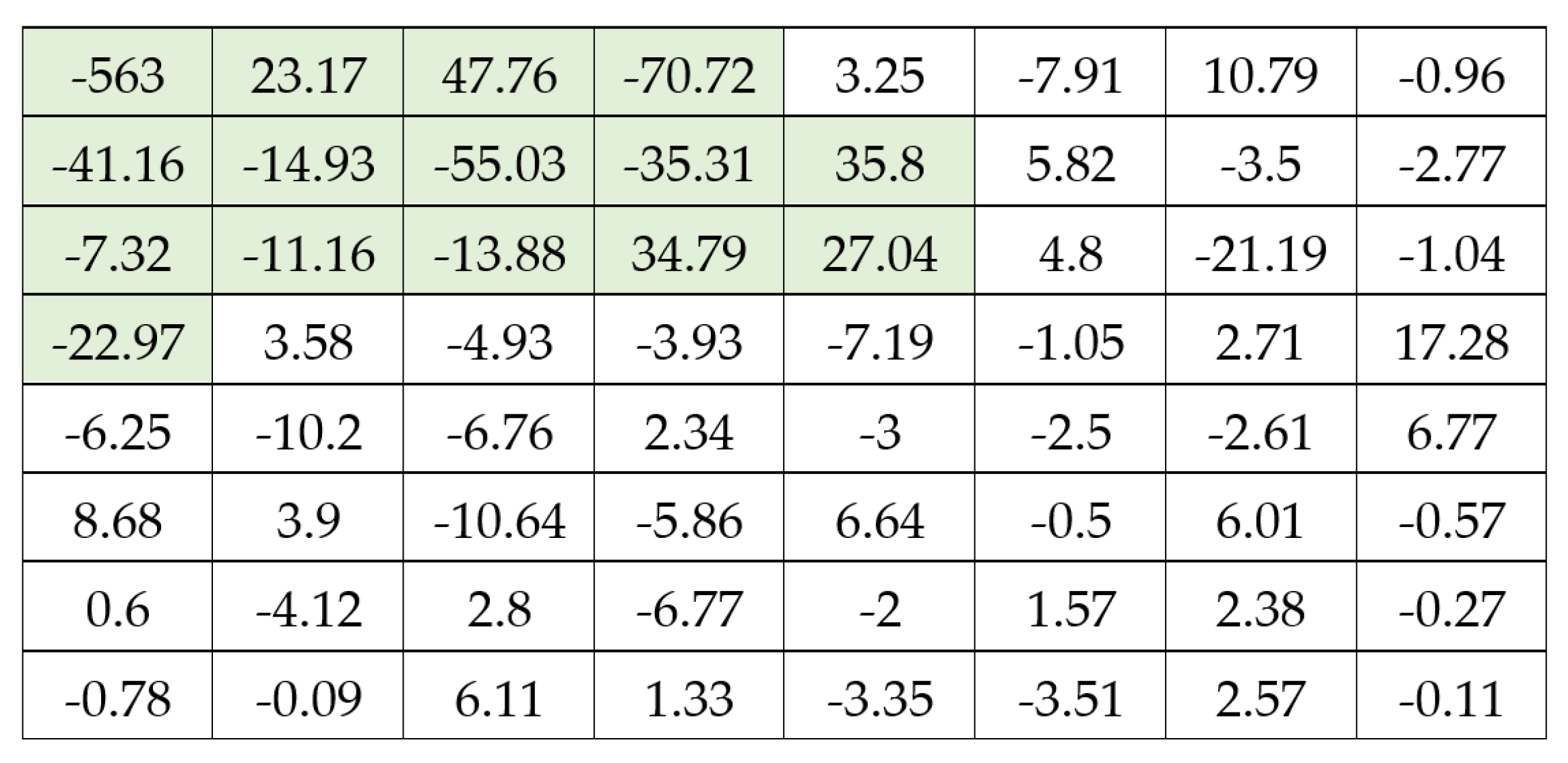
For a different quality factor, such as ${\mathrm{QF}}_1=60$, the property can be easily observed in an example, in

Table 5. Comparison between JPEG coefficients and the GBL, using Y channel.

Quality Factor for the Initial Compression QF1	Quality Factor for the Initial Compression QF2	Average p-Value for 100 Images
60	90	0
	80	0
	70	0.052688
	60	0.955229
	50	0.917083

. Thus, by establishing the threshold at p-value $\mathrm{n}=0.6$, suggested by the green line, the first ${\mathrm{QF}}_2$ under it, is ${\mathrm{QF}}_2=60$, which is indeed the second compression quality factor.

In fact, ${\mathrm{QF}}_2$ determined using this method has the property ${\mathrm{QF}}_2={\mathrm{QF}}_1$.

4. Discussion

Before moving further, it is important to restate that the developed algorithm finds the quality factor with which the image was compressed only once. The second quality factor is only applied by the algorithm in an incomplete second compression. Its only purpose is to obtain the JPEG coefficients (which is an intermediary step of JPEG compression).

In light of the abovementioned observations, we make the following complete statement. Given an input image, compressed with a quality factor ${\mathrm{QF}}_1\in \left\{90, 80, 70, 60, 50\right\}$, to determine it, the following algorithm can be applied:

• Calculate the JPEG coefficients for each ${\mathrm{QF}}_2\in \left\{90, 80, 70, 60, 50\right\}$, denoted by ${\mathrm{JPEG}}_{\mathrm{i} }$, $\mathrm{i}\in \left\{90, 80, 70, 60, 50\right\}$;
• For all coefficients, in relationship with the GBL, perform the chi square test and determine the p-values, denoted by ${\mathrm{p}}_{\mathrm{i}}$, $\mathrm{i}\in \left\{90, 80, 70, 60, 50\right\}$;
• If all ${\mathrm{p}}_{\mathrm{i}}$ satisfy the relationship ${\mathrm{p}}_{\mathrm{i}}>0.6$, the initial quality factor is ${\mathrm{QF}}_1=90$;
• Else, the largest ${\mathrm{QF}}_2$ for which ${\mathrm{p}}_{\mathrm{i}}>0.6$ is the initial quality factor ${\mathrm{QF}}_1={\mathrm{QF}}_2$.

In what follows, this property is exemplified on 100 images from the UCID, for each channel Y, R, G, and B, for ${\mathrm{QF}}_1\in \left\{90, 80, 70, 60, 50\right\}$. To represent graphically the outcome, the average p-values are calculated. Figure 14, Figure 15, Figure 16 and Figure 17 show the results. The threshold p-value is represented as a dashed red line for each case.

As it can be observed, the threshold p-value $\mathrm{n}=0.6$ represented by the red dashed line seems to be an appropriate choice for the algorithm. However, in

Table 6. The algorithm results for different threshold p-values, using Y channel.

Threshold p-Value	Number of Images	Channel from Which the JPEG Coefficients Are Extracted	Detection Accuracy for Each Original QF1					Overall Accuracy
			90	80	70	60	50
n = 0.5	500	Y	1	1	0.9	0.89	0.52	0.862
n = 0.6			1	1	0.9	0.87	0.61	0.876
n = 0.7			1	1	0.91	0.85	0.7	0.892
n = 0.8			1	1	0.88	0.83	0.72	0.886

, the results are shown for different threshold values. Random images are taken from the UCID database. They are compressed with different quality factors ${\mathrm{QF}}_1\in \left\{90, 80, 70, 60, 50\right\}$. Then, the abovementioned algorithm computes the quality factor ${\mathrm{QF}}_1$, using the JPEG coefficients obtained from the luminance channel. Besides the overall algorithm accuracy, we have also included the accuracies with which each original quality factor was determined.

Therefore, the threshold p-value is chosen to be $\mathrm{n}=0.7$ since it conducts to the best results for our algorithm.

Moreover, the accuracy of the algorithm decreases when detecting smaller quality factors. We believe that one of the reasons behind this is the parameters of the GBL. Tuning these parameters for our algorithm is a future goal.

However, the original algorithm only makes use of one channel, the luminance. Next, we use all four channels to predict the quality factor ${\mathrm{QF}}_1$. In this manner, if three of the four channels predict for example ${\mathrm{QF}}_1=60$ and one of the channels predicts ${\mathrm{QF}}_1=50$, the result is ${\mathrm{QF}}_1=60$.

As it can be observed from

Table 7. The algorithm results using Y, R, G and B channels.

Threshold p-Value	Number of Images	Channel from Which the JPEG Coefficients Are Extracted	Detection Accuracy for Each Original QF1					Overall Accuracy for One Channel	Overall Accuracy
			90	80	70	60	50
n = 0.7	500	Y	1	1	0.91	0.85	0.7	0.892	0.882
		R	1	1	0.92	0.82	0.52	0.852
		G	1	1	0.88	0.83	0.66	0.874
		B	1	1	0.84	0.74	0.44	0.804

, the accuracy of the algorithm cannot be improved in this manner. This is due to the fact that the luminance channel conducts to the best results, while the other channels have a negative impact on the predicted quality factor. Therefore, we have reached the conclusion that the algorithm, which uses the parameters of the generalized Benford’s law as they were presented in the previous sections, has the best performance when applied to the luminance channel while using a threshold p-value $\mathrm{n}=0.7$.

5. Conclusions

Summarizing, the above-described algorithm uses the JPEG coefficients from the luminance channel of already compressed JPEG images. It, therefore, determines the quality factor with which the analyzed images were compressed. Without using any means of machine learning, this algorithm reached an accuracy of 89% for 500 random images. Moreover, the algorithm had an accuracy of 100% when detecting the images compressed with quality factors 80 and 90.

As a final thought, we refer to the idea that “the numbers but play the poor part of lifeless symbols for living things” (Benford, 1938). In light of our research, we strongly believe that, when analyzed properly and meticulously, the numbers come alive, providing essential information. Such a case is the one of JPEG coefficients, which embed the traces of an image’s compression history.

Finally, it may be concluded that the methods of detecting the quality factor, such as the one presented above, along with the described properties of JPEG coefficients, are fundamental for developing deep learning algorithms used in image forensics. The results are presented in more details in the Discussion section of this article.

Moreover, we strongly believe that not only is the detection of a compromised image of great importance, but also the detection of the quality factor with which it was compressed.