1. Introduction
The laminated transformer core represents a problem domain that has very heterogeneous material characteristics. The most abrupt change in material characteristics is in the direction perpendicular to the lamination sheets, where thin ferromagnetic lamination sheets of high electrical conductivity and much thinner layers of electrical insulation occur alternately. On the other hand, the smoothest change in material characteristics is tangential to the lamination sheets. Therefore, the calculation of the eddy currents in a laminated core requires modeling on two different spatial scales [
1]. Because the transformer core typically consists of a large number of lamination sheets, the direct modeling of such a multiscale problem is practically unfeasible due to excessive demands on the computer’s working memory and the duration of the simulation [
2]. In order to reduce the computational requirements of the simulation, it is necessary to introduce certain approximations of the problem. One of the most common methodological steps is the homogenization of the material characteristics of the laminated core [
3]. Furthermore, due to the presence of different materials within the problem domain, there is a problem of discontinuous tangential and normal field components at the interfaces between different materials (e.g., air and iron) [
4]. In order to improve the accuracy of the calculation, instead of nodal basis functions that impose the complete continuity of the approximated vector field, edge basis functions that only impose the continuity of the tangential component of the approximated vector field are used [
5,
6].
In this paper, the focus is on open-type core transformers, which are commonly used for auxiliary power and rural electrification applications [
7]. Here, an open-type core transformer is used as a power transformer; thus, eddy current losses represent an important parameter in the open-type core design phase [
8,
9]. In order to reduce eddy current losses, the open-type core generally has a more irregular geometry and structure compared to the standard closed-type core, which further complicates the computer simulation of the eddy currents [
10].
2. Problem Definition
The problem domain consists of a simply connected laminated region and a surrounding eddy current free region , i.e., , with . The region has heterogeneous material characteristics, consisting of the electrically conductive ferromagnetic region and the electrical insulation region , where the . The region is laminated, consisting of n lamination sheets separated from each other by an extremely thin electrical insulation .
For this problem, a low-frequency range is assumed. Therefore, a magneto-quasi-static set of Maxwell’s equations is used, with the magnetic induction
and the eddy current density
as the fields of interest, and
as the source current density. Therefore, the set of equations for the modeling of eddy currents in
is as follows:
where
represents electrical resistivity and
ν represents magnetic reluctivity in
. The electrical resistivity
is a piecewise function in
, defined as
in
and
in
, where
is the resistivity of the lamination material, and
represents the resistivity of insulation, i.e.,
. Similarly, the magnetic reluctivity
is a piecewise function in
, defined as
in
and
in
, where
represents the reluctivity of the lamination material, which is assumed to be a linear ferromagnetic material, whereas
represents the reluctivity of the insulation material; thus,
.
Because
in the eddy current-free region
, the set of equations in
, in addition to (4), includes:
where
represents the magnetic reluctivity in
, and for simplicity
will be assumed below. For the source current density,
is possible only in
, i.e.,
is assumed in
.
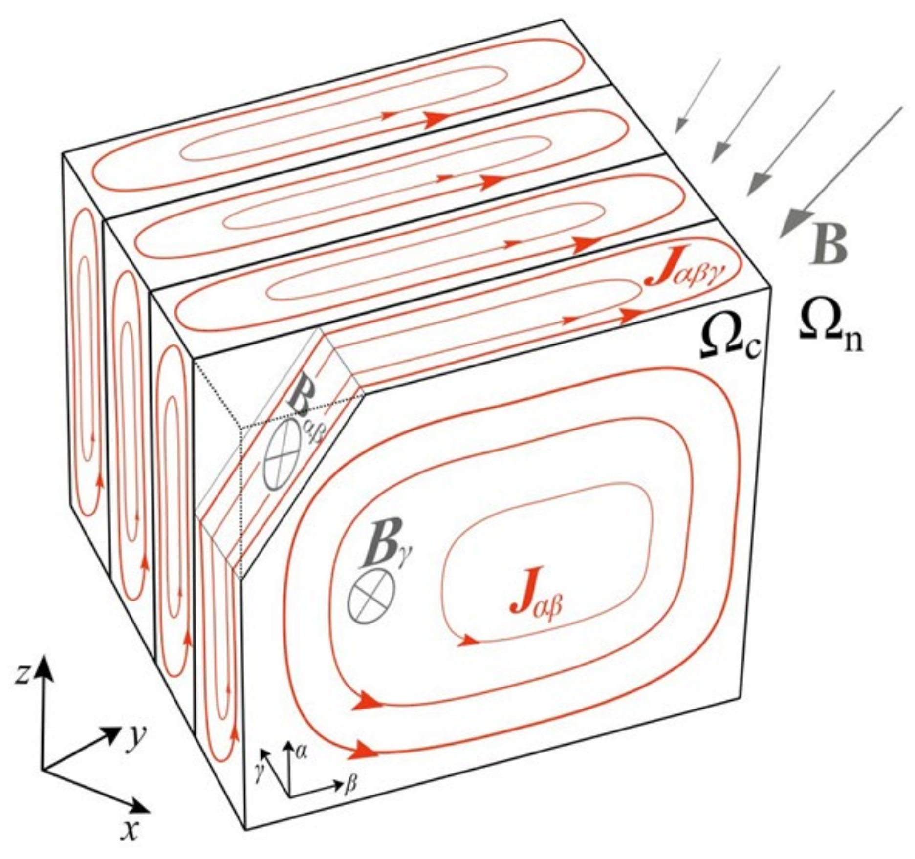
Eddy Currents in an Open-Type Core
The focus of the paper is on the open-type transformer core, which belongs to a set of simply connected laminated media, such as the one shown in
Figure 1. The problem of eddy currents in an open-type transformer core is characterized by certain specifications which are not necessarily present in the case of a closed-type transformer core. In the open-type core, eddy currents of density
are mostly concentrated in the outer lamination sheets. Furthermore, in the outer lamination sheets of the open-type core, eddy currents
are predominantly induced by the perpendicular component of the magnetic induction
, with respect to the lamination sheets. On the other hand, towards the interior of the open-type core, eddy currents
are predominantly induced by the tangential component of the magnetic induction
, with respect to the lamination sheets. It is then useful to separate the normal and tangential components of magnetic induction
and the eddy current density
in the calculation itself. Therefore, in the local orthogonal
αβγ-coordinate system of a single lamination sheet shown in
Figure 1, induction
can be written as the sum of the normal component
and the tangential component
with respect to the lamination sheet, that is
In accordance with (6), two corresponding equations follow from (1):
where
holds. According to (7), the component of the magnetic induction perpendicular to the lamination sheets induces the current density
, which only has tangential components with respect to the lamination sheets. On the other hand, the tangential component of magnetic induction, according to (8), induces eddy currents of density
which generally have all three spatial components, as shown in
Figure 1.
Although the
and
are coupled, it is a good approximation to simulate them separately [
11]. Because the value of magnetic permeability of the core is significantly lower in the perpendicular than in the tangential direction (with respect to the lamination sheets),
has a negligible effect on
, and consequently (according to (7)) a negligible effect on
.
Therefore, it is possible to ignore when calculating ; the reverse is not valid because the influence of on is not always negligible.
Because the open-type transformer core is surrounded by a medium of low magnetic permeability (air), a large proportion of the total magnetic flux enters the core perpendicular to the lamination sheets; thus,
is usually several times larger than
in the outer lamination sheets, which further reduces the importance of considering
when calculating
. Therefore, in contrast to the closed-type core, the losses due to
usually represent a major part of the total eddy current losses in the open-type core [
12,
13]. In this paper, the emphasis is therefore on the method of calculating the eddy current density
, i.e., losses due to
. Hence,
will be neglected in the first simulation step when calculating
, and it can be calculated in the second simulation step [
14,
15], or only the losses due to
can be calculated in the post-processing [
3].
3. Specifications of the Laminated Open-Type Core
As previously described, in the case of the open-type core,
usually has a significantly higher value in the outer lamination sheets compared to
, and the total eddy current losses due to
are several times larger than the total losses due to
. In order to reduce the value of
, it is desirable to reduce the surface area of the lamination sheets. Some of the engineering options are to assemble the open-type core from several smaller, more slender lamination stacks, and/or to use heterogeneous stacking directions for the lamination sheets [
10,
16].
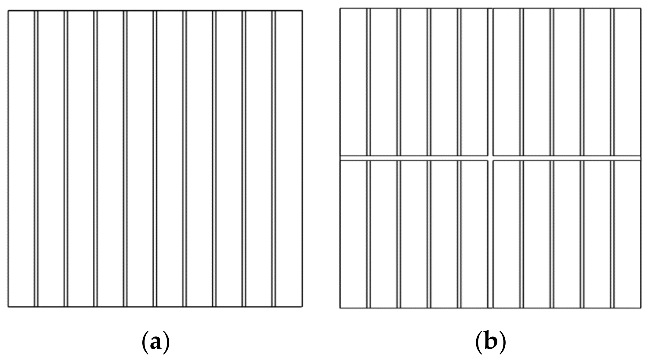
Figure 2 shows a comparison of the cross-sections of the standard (one-part) core and the multipart core composed of four slenderer cores.
The
region of the open-type core shown in
Figure 2a is without region partitions, i.e.,
, as denoted in
Figure 3a. On the other hand, the
region of the multipart open-type core shown in
Figure 2b consists of the individual parts of the core
, where every two adjacent parts of the core
and
are mutually isolated by an insulation layer
, i.e.,
, as denoted in
Figure 3b.
Again, as in the case of a standard one-part open-type core, each part of the multipart core consists of a laminated ferromagnetic part
and the associated insulation region
, that is,
. Because the open-type core is topologically simply connected, some other configurations of the parts of the multipart core in
Figure 2b are easily feasible. To enable open-type transformer core optimization, the developed method should be able to simulate eddy currents for all possible configurations.
4. Homogenization of the Laminated Open-Type Core
An extremely dense finite element mesh, especially in the
γ-direction, can be avoided by homogenizing the material characteristics of the
region, thus obtaining the
region. The homogenization of the electrical and magnetic characteristics of a laminated medium with a fill factor
yields the anisotropic characteristics of the material, with the diagonal tensors of electrical resistivity
ρ and magnetic reluctivity
ν being defined as
As was already stated, only (2) and (7) are modeled in the first simulation step, whereas the fields in (8) are neglected. The values of all of the fields in (2) and (7) change monotonically in the
γ-direction, and therefore the components of
ρ and
ν defined in (9) and (10) are calculated using the following well-known Formula [
11]:
Note that, due to (12), eddy current density goes approximately to zero, and consequently, the fields in (8) will approximately be equal to zero.
In the case of a multipart open-type core,
region homogenization is carried out by applying (9)–(14) to each
part of the multipart core separately, with interface surfaces
instead of
layers between them. Therefore, each homogenized part
will be assigned its
and
tensors. However, for the thin insulating region
to be homogenized and modeled as the interface surface
between the two adjacent core parts (
and
region), at least one of the two core parts must have a component of the tensor
equal to zero in the direction perpendicular to the interface surface
, in order to prevent the flow of eddy currents from
to the
region. If this is not the case, the direct modeling of
is one of the options. However, a much denser mesh within and around the
region is then needed, which significantly slows down the simulation convergence. For the multipart core shown in
Figure 2b, i.e., in
Figure 3b, regions
and
cannot be modeled as
and
.
A much more economical and simpler approach is to use a formulation based on the current vector potential
, approximated by the edge elements. In this case, instead of the direct modeling of the insulation regions
, it is possible to only prescribe the interface condition
on the surface
between two parts of the multipart core, where
is perpendicular to the surface
. This ultimately prevents the penetration of eddy currents from one part of the core into another, because
holds. Hence, a
-based formulation, such as a
formulation, is a better choice for the modeling of eddy currents in an open-type laminated core, where
φ represents the magnetic scalar potential. On the other hand, the
formulation does not ensure the exact continuity of the magnetic induction component
at the interface between the core and the surrounding air, but this continuity is ensured only in a weak sense. This is a problem, because to accurately calculate
, according to (4), it is necessary to accurately calculate
. If the magnetic vector potential
, approximated by the edge elements, is used instead of
φ, the continuity of
at the air-core interface is ensured in a strong sense. Therefore, a method for the calculation of the eddy currents described in this paper will be based on the
formulation, which uses
and
in the core, and only
in the surrounding region [
17,
18].
5. The Weak Formulation
According to (3) and (4), the current density
and magnetic induction
are solenoidal fields, so it follows that
and the source current density
is also a solenoidal field, so it holds that
In order to ensure the consistency of the left-hand side and the right-hand side of the future matrix, Equation (17) will be used instead of
[
19]. By including (15)–(17) in (1) and (2), a formulation of the eddy current problem in
is obtained as:
Similarly, by including (16) and (17) in (5), a formulation in
follows:
As shown in
Figure 4, region
is enclosed by surface
, which represents the interface between regions
and
. The interface conditions between the fields in
and
must be satisfied on
, i.e.,
where the exponents “
n” and “
c” denote fields in the
and
parts of the domain, respectively. The continuity of the normal component of magnetic induction
is exactly preserved, because
is approximated with edge elements, i.e., (21) is automatically satisfied at
. Condition (22) can be written as
, i.e., it is necessary to prescribe the interface condition on
as
Because
by definition, from (23) it follows that
, and using (15) it follows that
. The boundary condition is then prescribed on
as
The boundary conditions must also be defined on
and
, where
and
are the disjointed outer boundaries of
, as shown in
Figure 4. The surface
represents the surface on which (26) holds, while
represents the surface on which (27) holds, i.e.,
For the sake of conciseness and without a lack of generality, it will be assumed below that
is not present, i.e., the entire outer surface of
is
. The boundary condition (26) is valid for a sufficiently distant boundary
. Because
holds, from (26) it follows that the homogeneous Dirichlet boundary condition on
is
In order for the coefficient matrix to be symmetric, a time-primitive vector field
is used instead of
, i.e.,
[
20]. Using (19), (20) and interface condition (24), the first equation of the weak
formulation is obtained:
From (18) follows the second equation of the weak
formulation:
In (29) and (30), represents both the edge basis functions (for the interpolation of and ) and weighting functions. Notice that the coefficient matrix for the weak Galerkin formulation (29) and (30) makes a consistent and symmetric system of equations.
6. Elimination of Degrees of Freedom
Because the formulation uses two vector potentials in , the total number of degrees of freedom in is , where represents the total number of edges in the finite element mesh in . This is significantly more degrees of freedom compared to the formulations that use one vector and one scalar potential in and have a total of degrees of freedom in , where is the number of nodes in the finite element mesh in . A higher number of degrees of freedom adversely affects the working memory and duration of the simulation.
Because
is neglected when calculating
, the current vector potential
should only define
in (15). Thus, in an orthogonal
αβγ-coordinate system defined locally within a lamination sheet, where the
γ-direction represents the normal direction of the lamination sheet, (15) can be written as
As can be seen from (31), only
is needed, whereas the tangential components
and
are zero, and therefore redundant. If the right prismatic finite elements (wedge or hexahedron) with the base parallel to
αβ plane and the height aligned with the
γ-direction are used, then it is possible to geometrically decouple the degrees of freedom associated with the
component from the degrees of freedom associated with the
and
components, as shown in
Figure 5. Because
is interpolated with edge basis functions, the degrees of freedom associated with the edges lying in the
γ-direction then approximate only the
component, and the degrees of freedom associated with the edges belonging to the base of the element approximate
and
components.
In
Figure 5,
represents the degree of freedom associated with edge
, and is calculated as a line integral of the current vector potential
along
. Because each edge of a finite element is assumed to be either aligned with the
γ-direction or parallel to the
αβ plane, it is associated with either
or
. If the
edge is aligned with the
γ-direction, then it is associated with
degree of freedom:
On the other hand, if the
edge is parallel to the
αβ plane, then
follows as:
Because the
and
components are equal to zero, each
degree of freedom should be equal to zero. In order to achieve this, surface condition
, which implies that
and
, can be given on the basis of the prismatic finite elements.
Figure 6a shows a sequence of the prismatic (wedge) finite elements extruded in the
γ-direction in three layers between the two interface surfaces
.
In order to set the surface condition
on the bases of finite elements, the tangential surfaces associated with the element bases are extruded together with the finite elements, as shown in
Figure 6b. Thus, all of the
degrees of freedom belong to one of the created tangential surfaces, as denoted by
. Because setting
on
fixes the values of
degrees of freedom to
, two-thirds of the total number of
degrees of freedom are eliminated from the simulation.
In addition, (12) becomes redundant, i.e., the anisotropy of the electrical resistivity is already ensured by setting on the surfaces.
8. Conclusions
The open-type core has certain differences with respect to the closed-type core that are important when calculating eddy current losses. Because the eddy currents in a real-size open-type core are largely induced by the magnetic induction component perpendicular to the lamination sheets, the open-type core may have a multi-part structure in order to reduce the eddy current losses. In addition, fields and eddy current losses are mostly located in the outer lamination sheets, such that the design optimization of an open-type core may require even more irregular geometry. Consequently, the complete homogenization of such a core is often not possible. Despite a significantly higher number of degrees of freedom, the formulation offers the greatest flexibility in the optimization of the open-type transformer core with respect to eddy current losses. By creating an appropriate geometric model and FE mesh, it is possible to eliminate the redundant degrees of freedom of the current vector potential , thus significantly improving the convergence rate of the eddy current simulations. Additionally, by eliminating the degrees of freedom in the formulation, it is also possible to prescribe the anisotropic electrical conductivity of an open-type core with heterogeneous lamination stacking directions and/or curved lamination sheets, assuming that they are simply connected. In future work, the ATAΓt method will be extended to the nonlinear case, and a comparison of the simulation results with the measurements will be made.


