1. Introduction
High-speed trains have been competitively developed worldwide since the first line was launched in Japan in 1964. The competition has been even more accelerated after the running speed of the French high-speed train TGV V150 exceeded 574.8 km/h. Because a faster cruising speed manifests technological superiority over others, many relevant studies have been carried out between worldwide manufacturers to develop faster trains. However, as the cruising speed of high-speed trains increases, noise emission also increases, and the aerodynamic noise contributes more significantly than the traditional rolling noise [
1,
2,
3,
4].
On the European market, the noise emission of high-speed trains for the community is limited by the technical specification for interoperability (TSI), which encourages train manufacturers to implement noise assessment early in the design phase. The experimental techniques can be applied either in scaled models in wind tunnels or full-scale running trains [
5,
6,
7,
8].
However, experimental results obtained from scaled models have difficulty in accurately representing real trains or actual operating conditions. By the way, full-scale testing under actual conditions can provide accurate information, but is unlikely to be possible in the design process. Furthermore, relying entirely on this late and expensive approach can add significant development costs and time to dealing with noise issues. For this reason, accurate numerical prediction of aerodynamic noise is very valuable in that it allows for noise assessment and improvement of full-scale trains at an early stage, sufficient to influence the design.
Recently, numerical studies [
9,
10,
11,
12,
13] were carried out on the aerodynamic noise of high-speed trains. In general, it has been reported that the first bogie, the pantograph, and the inter-coach space, are the primary aerodynamic noise sources of high-speed trains. However, these studies used a simplified body model or only a single part. Meskine et al. [
14] performed hybrid computational aeroacoustic simulations on a full-scale geometry of a high-speed train to estimate the flow-induced noise contribution radiated to the far-field. However, this study focused only on externally radiated noise, which is relevant to rail transportation community noise.
The interior noise of a high-speed train due to external flow disturbance is also one of the critical issues for product developers to consider during a design state. The external surface pressure field induces the vibration of the wall panels of a high-speed train, and this vibration generates the interior sound. Therefore, it is the first step for low interior noise design to characterize the surface pressure fluctuations. The fluctuating surface pressure field consists of two distinct components: incompressible (or hydrodynamic) and compressible (or acoustic) pressure fields. Given that the incompressible pressure wave induced by the turbulent eddies within the boundary layer is transported approximately at the mean flow speed and the compressible pressure wave propagates at the vector sum of the sound speed and the mean flow velocity, the transmission characteristics of hydrodynamic and acoustic pressure waves through the wall panel of the cabin are pretty different from each other. Lee et al. [
15] computed the flow field around a high-speed train at the speed of 300 km/h in an open field by employing a highly accurate LES technique with high-resolution meshes of more than 300 million grids. The unsteady surface pressure fields were then decomposed into the incompressible and compressible ones using the wavenumber-frequency transform (WFT), and the surface pressure power spectral levels due to each wall pressure fluctuations were estimated and compared for the selected wall panels of the train. These results showed that the incompressible pressure components contribute more to the total surface pressure levels in the low-frequency range, whereas the compressible ones do more in the high-frequency range. This fact implies that the interior sound of a high-speed train also follows the same spectral characteristics. Accordingly, the measure for reducing the interior sound may differ according to the frequency range because the speeds of compressible surface pressure waves are much higher than the incompressible ones.
There are many tunnels for high-speed rail in mountainous areas. For example, the Seoul–Busan high-speed line in Korea consists of 412 km of double tracks, including 191 km (46%) of tunnels [
16]. Given that cabin interior noise generally increases when a high-speed train passes through a tunnel, developing high-speed trains with quieter interior noise in such an environment is more critical.
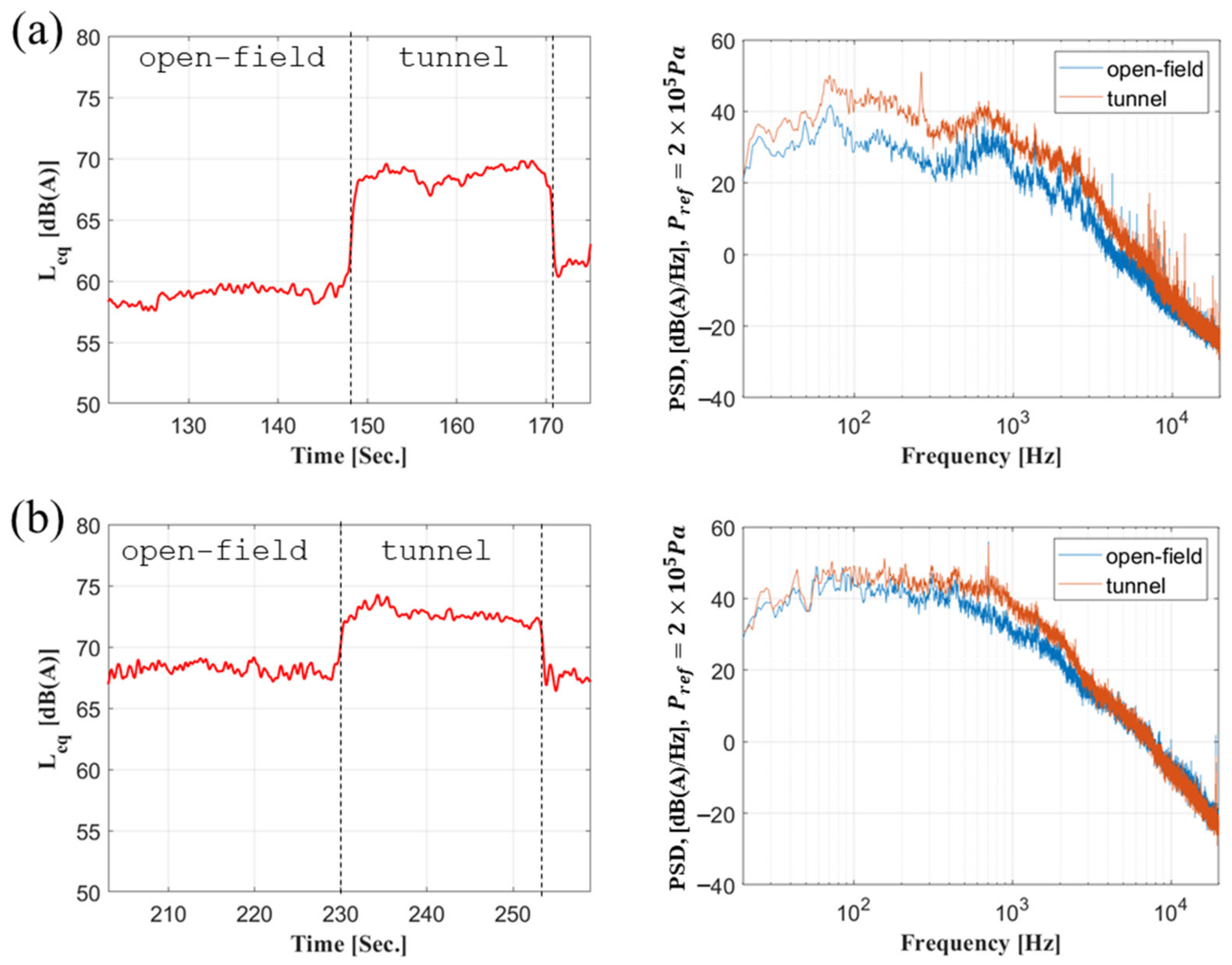
Figure 1 shows the time histories of the overall sound pressure levels measured inside coaches of two high-speed trains running both in open-field and tunnels with integration time 0.5 s. The averaged running speeds of the trains when the measurements were carried out are listed with averaged SPLs (sound pressure levels) in
Table 1. It has been observed that the sound pressure levels measured in cabins while the trains are running inside tunnels are higher by about 5 dB to 10 dB than those in open-field [
17]. The sound sources contributing to high-speed train interior noise can be classified into three categories: equipment noise, structure-borne noise, and airborne noise. HVAC (heating, ventilation, air conditioning) systems are mainly responsible for the equipment noise. Structure-borne noise is caused by the reradiation from the structures excited by vibroacoustic sources like wheel/rail contact and engine/auxiliary equipment. Lastly, as described above, the airborne noise is due to external flow disturbances that can be further divided into incompressible and compressible pressure fields. The surface pressure fields drive the vibration of the body panels and windows of a high-speed train, thereby causing interior sound. The strength of the source causing the equipment and structure-borne noises is not different between open field and tunnel, and thus the difference in the sound pressure levels measured in a cabin is mainly due to the external flow disturbances.
This study aims to investigate the leading cause of the difference observed in the sound pressure levels measured inside the cabin of high-speed trains cruising in an open field and in a tunnel. The characteristics of surface pressure fluctuations are analyzed by assessing relative contributions between the incompressible and compressible wall pressure fluctuations. First, compressible LES (large eddy simulation) techniques with high-resolution grids are employed to accurately and simultaneously predict the exterior flow and acoustic fields around a high-speed train. The high-speed train targeted in this study is the EMU-320, a high-speed multiple-unit train manufactured by Hyundai Rotem and planned to be operated by Korail in 2025. The high-speed train is assumed to cruise at 300 km/h in open-field and tunnel, respectively. The cross-sectional shape of the tunnel is also determined by using the existing tunnel. The predicted fluctuation pressure field in the wall panel surface of a train is decomposed into incompressible and compressible ones using the WFT. Lastly, the power levels due to each pressure field are computed and compared between open-field and tunnel.
The main contributions of the present study are three-fold. The first is to clarify the origin of the increased interior sound of a high-speed train running in a tunnel compared to in an open field. There is no noticeable difference in the power levels of incompressible surface pressure fluctuations between the two cases. However, the decomposed compressible one in the tunnel case is higher by about 2~10 dB than in the open-field case. This result implies that the strength of aerodynamic sound sources of a high-speed train is not significantly different between an open field and tunnel, but the sound pressure levels are increased in the tunnel operation condition because the generated sound pressure is confined with a tunnel. The second is to clarify the importance of compressible surface pressure field in terms of the origin of the interior sound of a high-speed train. The power levels of total surface pressure are similar between the two operating conditions; however, as described above, the power levels of compressible pressure are higher in a tunnel than in an open field. However, the magnitudes of spectral power levels of compressible pressure are still lower than those of incompressible pressure. Despite the difference in magnitudes between the two pressure fields, the measured interior sound pressure levels are more correlated with predicted compressible pressure, which manifest the effective transmission of the compressible pressure field. This can be understood as the fact that subsonic surface waves support only evanescent waves in a fluid that is always confined to the interface’s vicinity. The third is to provide the spectral power levels of total, incompressible and compressible wall pressure fluctuations for all of the wall panels of coaches of a high-speed train, which can be used as input data to calculate interior sound via vibroacoustic solvers in a related future study.
The structure of the present paper is organized as follows. In
Section 2, the governing equations and numerical methods for simulating the external flow of a high-speed train are described, and the WFT used for decomposing the predicted surface pressure field into the incompressible and compressible ones are presented. The geometry of the target train and the computational conditions and domains are detailed. In
Section 3, the predicted flow fields around the high-speed trains are analyzed to focus on the different operating conditions of the open field and tunnel.
Section 4 investigates primary aerodynamics noise sources such as the bogies, the pantographs, and the HVAC box. In
Section 5, the wavenumber-frequency analysis is illustrated for the surface pressure field on the selected roof and the sidewall surfaces of a high-speed train. In
Section 6, the predicted incompressible and compressible surface pressure fields and their power spectrum are presented for all of the surfaces of a high-speed train and compared between an open field and a tunnel.
3. Unsteady Flow Analysis
Figure 6 shows the snap-shot of velocity magnitude contours at the central vertical plane for both cases. In both cases, results can be seen a significant reduction in the velocity magnitude is induced in the first bogie under the body and the separated flows cover the downstream coaches behind the TC-car. However, the flow pattern upstream and downstream of the train is slightly different between the two cases: disturbed velocity fluctuations exist in more upstream and downstream directions for the tunnel case. These results can be understood as the disturbances occurring around the vehicle body are more trapped in the tunnel than in the open field.
Figure 7 shows the instantaneous static pressure field on the same plane for both cases as
Figure 6. It can be seen in
Figure 7a for the open-field case that the compressible acoustic pressure waves propagate from the train bodies, and the primary aeroacoustic sources are the bogies, pantographs, inter-coach gaps, and roof fairings. However, for the tunnel case in
Figure 7b, the acoustic pressure waves generated from the train are confined by the tunnel and seem to form a more complex pattern due to their interaction with the hydrodynamic fluctuation. These differences are more highlighted in
Figure 8, which shows the instantaneous iso-contours of pressure fluctuations
defined as
on the horizontal plane at the height of 1.5 m from the ground and at the central vertical plane. The circular radiation patterns of the compressible acoustic pressure waves from the well-known aerodynamic noise sources, such as bogies, pantographs, and inter-coaches were more clearly visible in the open-field case. However, in the tunnel case, those patterns seemed to be more complex due to the interaction of acoustic pressure waves with the tunnel wall and the hydrodynamic field.
For more quantitative analysis, the pressure coefficient defined as
where
is the upstream pressure,
is the time-averaged static pressure,
is the air density, and
is the train speed, is computed on the train surface.
Figure 9a,b show the distributions of the computed pressure coefficient on the lines where the train surface meets the planes of y = 0 and z = 1.107 m, respectively, for the train in the open field. The monitored lines are also depicted using the red- and blue-colored lines and the black-colored lines on the train surface. There is the most significant variation in the pressure distribution around the train head because the flow decelerates in the vicinity of the stagnation point of the train head nose and again accelerates in the downstream direction along the surface of the train head. The process is reversed for the flow around the train tail, with a negative peak followed by a positive peak. It can also be seen that the parts where the significant pressure variation occurs match the vital source regions, as shown in
Figure 8a.
In the upper side of the train, as shown in
Figure 9a, the substantial variations in the pressure coefficient occur around the following parts: the front nose and HVAC boxes of the TC-car, the pantograph and the HVAC box of the M1-car, the HVAC box and pantograph of the M’3-car, and the HVAC boxes of the TC2-car. Significantly, the pressure variation on the rear part of the M’3-car is as high as that of the train head because the pantograph goes up, thereby manifesting the most contributing aerodynamic noise source. In the gap region between the train body and the ground, as shown in
Figure 9a, the significant variation in pressure occurs in the bogie parts, which are also known to be one of the most critical aerodynamic noise sources. Significantly, the pressure is lowest in the first bogie of the TC-car. The variation pattern of pressure coefficient along the sidelines, as shown in
Figure 9b, is similar to the bottom line, since the sidelines are also located near the bogies. The locations where the most significant pressure variation occurs match those of bogie cavities.
Figure 10a,b show the distributions of the computed pressure coefficient on the lines where the train surface meets the planes of y = 0 and z = 1.107 m, respectively, for the train in the tunnel. Overall, characteristics of the pressure variation are very similar to those of the train in the open field. This result implies that the primary aerodynamic noise generation mechanism over the train running in a tunnel is similar to that in open space.
5. Decomposition of Surface Pressure Fields
The WFT is applied to the unsteady wall pressure fluctuations on the external walls of the train to decompose those into the compressible and incompressible pressure fields. The illustrative WFT is conducted by applying Equation (12) to wall pressure fluctuations on the sidewall of the TC-car depicted in
Figure 18. The coordinate system for the wavenumber-frequency analysis is shown in
Figure 18 and
Figure A1 (in
Appendix A). The train running in the open field is considered. The sampling rate
and the frequency interval ∆
f were 5000 Hz and 4.88 Hz, respectively. The power spectral density obtained from the wavenumber-frequency transform of the pressure field on Plane-A in
Figure 18 is plotted in
Figure 19. The slanted Dirac cone (
) and the convected incompressible pressure can be distinctly identified. To highlight the characteristics of the 3-D PSD diagram more clearly, the 2-D PSD diagram at the plane of
is shown on the right side of
Figure 19. Significant compressible components are identified between the characteristic lines of which the slopes correspond to the phase speeds of
and
, while the most incompressible components are located around the characteristic line of slope
.
These distinctly separated regions manifest that the LES effectively captures the aerodynamic noise generation and the acoustic wave propagation in the external flow field of the high-speed train.
Figure 20a shows the PSD of the total, compressible, and incompressible pressure fields. The spectrum of the compressible and incompressible pressure is obtained by applying the following formula,
The results demonstrate that the incompressible pressure components dominate in most of the frequency range, except for 122.1 Hz, below 1 kHz. Generally, the incompressible components dominate in the low-frequency range while the compressible ones in the high-frequency range. However, the tonal component around 122.1 Hz is found to be due to compressible pressure from the decomposed pressure spectrum.
Figure 20b shows the snapshot of the compressible and incompressible wall pressure fluctuations reconstructed by applying the inverse WFT to the incompressible and compressible regions separately. It can be seen that the compressible pressure fields form the wave pattern with a larger wavelength, which implies a higher wave speed than the incompressible pressure one that convects approximately at the cruising speed of the train.
The wavenumber-frequency analysis is also conducted on the surface pressure fields on the wall planes denoted by the symbols B and C in
Figure 21.
Figure 22 shows the wavenumber-frequency diagrams of surface pressure fields and the corresponding PSD levels of total, compressible, and incompressible pressure for the [lanes of B and C, which are selected due to their proximity to the first bogie, the HVAC box, and the second pantograph, respectively, which are identified as the primary aerodynamic noise sources. It can be seen in
Figure 22 that the tonal components can be observed in the decomposed compressible pressure spectra, whereas any of them cannot be found in the total pressure spectra. The tonal component at 127.0 Hz, which is associated with the bogie and the HVAC box, can be found in the PSD of the compressible pressure field on Plane-B in
Figure 22a. The tonal peak at 190.4 Hz observed in the flow field around the raised pantograph can also be identified in the compressible pressure spectrum of
Figure 22b. The slight differences observed in the tonal frequencies between the filtered pressure fluctuations in
Figure 12,
Figure 16 and
Figure 17 and the wavenumber-frequency diagram in
Figure 22 are due to their different frequency resolutions.
7. Conclusions
In this study, the characteristics of fluctuating surface pressure on the high-speed train, EMU320 cruising at the speed of 300 km/h in an open field and a tunnel were investigated by using the high-resolution LES technique combined with the wavenumber-frequency analysis. First, the external flow field, including compressible acoustic components, around the EUM320 was computed using the compressible LES with approximately 600-million grid cells. The predicted flow field results clearly revealed the dominant aerodynamic source regions: the first bogies, the raised pantographs, and the HVAC box. There was no noticeable difference between the open field and tunnel running conditions in terms of total pressure distribution, except that the aerodynamic noise radiated from the above-described sources of the train running in the tunnel was confined inside the tunnel. To decompose wall pressure fluctuations into incompressible and compressible ones, the WFT was performed on wall pressure fluctuations of the train. The tonal components associated with the primary aerodynamic noise sources could be identified in the decomposed compressible pressure spectra, whereas any of them could not be found in the total pressure spectra. Finally, the decomposed incompressible and compressible wall pressure fluctuations between the two cases were compared in terms of PSD levels. The predicted PSD levels of compressible pressure fluctuations in the case of a train cruising in the tunnel were higher by about 2 dB to 10 dB than that of a train running in an open field, while there was no significant difference in the level of incompressible pressure fluctuations between the two cases. Predicted differences properly matched those measured in cabins of high-speed trains in service. These results revealed that the increased interior noise levels of high-speed trains running in a tunnel were mainly due to compressible pressure fields though their magnitudes were less than incompressible ones, which implied that the effective measure to suppress interior noise must focus on the increase of transmission loss of sound waves through the panels of high-speed trains.
Future studies should aim to incorporate the decomposed acoustic and hydrodynamic wall pressure fluctuations for the prediction of interior cabin noise of the high-speed train. The result can be utilized to assess the relative contributions of the acoustic and hydrodynamic wall pressure fluctuations to the interior noise and thus help develop an effective design of cabin structure to reduce interior noise.


