Article

Comparative Analysis of Surface Pressure Fluctuations of High-Speed Train Running in Open-Field and Tunnel Using LES and Wavenumber-Frequency Analysis

1
School of Mechanical Engineering, Pusan National University, Busan 46241, Yeongnam, Korea
2
Applied Technology Research Team, Hyundai Rotem Company, 37 Cheoldobangmulgwan-ro, Uiwang-si 16082, Gyeonggi-do, Korea
*
Author to whom correspondence should be addressed.
Appl. Sci. 2021, 11(24), 11702; https://doi.org/10.3390/app112411702 (registering DOI)
Submission received: 27 October 2021 / Revised: 18 November 2021 / Accepted: 7 December 2021 / Published: 9 December 2021
(This article belongs to the Section Acoustics and Vibrations)

Abstract

:
The interior noise of a high-speed train due to the external flow disturbance is more than ever a major problem for product developers to consider during a design state. Since the external surface pressure field induces wall panel vibration of a high-speed train, which in turn generates the interior sound, the first step for low interior noise design is to characterize the surface pressure fluctuations due to external disturbance. In this study, the external flow field of a high-speed train cruising at a speed of 300 km/h in open-field and tunnel are numerically investigated using high-resolution compressible LES (large eddy simulation) techniques, with a focus on characterizing fluctuating surface pressure field according to surrounding conditions of the cruising train, i.e., open-field and tunnel. First, compressible LES schemes with high-resolution grids were employed to accurately predict the exterior flow and acoustic fields around a high-speed train simultaneously. Then, the predicted fluctuating pressure field on the wall panel surface of a train was decomposed into incompressible and compressible ones using the wavenumber-frequency transform, given that the incompressible pressure wave induced by the turbulent eddies within the boundary layer is transported approximately at the mean flow and the compressible pressure wave propagated at the vector sum of the sound speed and the mean flow velocity. Lastly, the power levels due to each pressure field were computed and compared between open-field and tunnel. It was found that there is no significant difference in the power levels of incompressible surface pressure fluctuations between the two cases. However, the decomposed compressible one in the tunnel case is higher by about 2~10 dB than in the open-field case. This result reveals that the increased interior sound of the high-speed train running in a tunnel is due to the compressible surface pressure field.

1. Introduction

High-speed trains have been competitively developed worldwide since the first line was launched in Japan in 1964. The competition has been even more accelerated after the running speed of the French high-speed train TGV V150 exceeded 574.8 km/h. Because a faster cruising speed manifests technological superiority over others, many relevant studies have been carried out between worldwide manufacturers to develop faster trains. However, as the cruising speed of high-speed trains increases, noise emission also increases, and the aerodynamic noise contributes more significantly than the traditional rolling noise [1,2,3,4].
On the European market, the noise emission of high-speed trains for the community is limited by the technical specification for interoperability (TSI), which encourages train manufacturers to implement noise assessment early in the design phase. The experimental techniques can be applied either in scaled models in wind tunnels or full-scale running trains [5,6,7,8].
However, experimental results obtained from scaled models have difficulty in accurately representing real trains or actual operating conditions. By the way, full-scale testing under actual conditions can provide accurate information, but is unlikely to be possible in the design process. Furthermore, relying entirely on this late and expensive approach can add significant development costs and time to dealing with noise issues. For this reason, accurate numerical prediction of aerodynamic noise is very valuable in that it allows for noise assessment and improvement of full-scale trains at an early stage, sufficient to influence the design.
Recently, numerical studies [9,10,11,12,13] were carried out on the aerodynamic noise of high-speed trains. In general, it has been reported that the first bogie, the pantograph, and the inter-coach space, are the primary aerodynamic noise sources of high-speed trains. However, these studies used a simplified body model or only a single part. Meskine et al. [14] performed hybrid computational aeroacoustic simulations on a full-scale geometry of a high-speed train to estimate the flow-induced noise contribution radiated to the far-field. However, this study focused only on externally radiated noise, which is relevant to rail transportation community noise.
The interior noise of a high-speed train due to external flow disturbance is also one of the critical issues for product developers to consider during a design state. The external surface pressure field induces the vibration of the wall panels of a high-speed train, and this vibration generates the interior sound. Therefore, it is the first step for low interior noise design to characterize the surface pressure fluctuations. The fluctuating surface pressure field consists of two distinct components: incompressible (or hydrodynamic) and compressible (or acoustic) pressure fields. Given that the incompressible pressure wave induced by the turbulent eddies within the boundary layer is transported approximately at the mean flow speed and the compressible pressure wave propagates at the vector sum of the sound speed and the mean flow velocity, the transmission characteristics of hydrodynamic and acoustic pressure waves through the wall panel of the cabin are pretty different from each other. Lee et al. [15] computed the flow field around a high-speed train at the speed of 300 km/h in an open field by employing a highly accurate LES technique with high-resolution meshes of more than 300 million grids. The unsteady surface pressure fields were then decomposed into the incompressible and compressible ones using the wavenumber-frequency transform (WFT), and the surface pressure power spectral levels due to each wall pressure fluctuations were estimated and compared for the selected wall panels of the train. These results showed that the incompressible pressure components contribute more to the total surface pressure levels in the low-frequency range, whereas the compressible ones do more in the high-frequency range. This fact implies that the interior sound of a high-speed train also follows the same spectral characteristics. Accordingly, the measure for reducing the interior sound may differ according to the frequency range because the speeds of compressible surface pressure waves are much higher than the incompressible ones.
There are many tunnels for high-speed rail in mountainous areas. For example, the Seoul–Busan high-speed line in Korea consists of 412 km of double tracks, including 191 km (46%) of tunnels [16]. Given that cabin interior noise generally increases when a high-speed train passes through a tunnel, developing high-speed trains with quieter interior noise in such an environment is more critical. Figure 1 shows the time histories of the overall sound pressure levels measured inside coaches of two high-speed trains running both in open-field and tunnels with integration time 0.5 s. The averaged running speeds of the trains when the measurements were carried out are listed with averaged SPLs (sound pressure levels) in Table 1. It has been observed that the sound pressure levels measured in cabins while the trains are running inside tunnels are higher by about 5 dB to 10 dB than those in open-field [17]. The sound sources contributing to high-speed train interior noise can be classified into three categories: equipment noise, structure-borne noise, and airborne noise. HVAC (heating, ventilation, air conditioning) systems are mainly responsible for the equipment noise. Structure-borne noise is caused by the reradiation from the structures excited by vibroacoustic sources like wheel/rail contact and engine/auxiliary equipment. Lastly, as described above, the airborne noise is due to external flow disturbances that can be further divided into incompressible and compressible pressure fields. The surface pressure fields drive the vibration of the body panels and windows of a high-speed train, thereby causing interior sound. The strength of the source causing the equipment and structure-borne noises is not different between open field and tunnel, and thus the difference in the sound pressure levels measured in a cabin is mainly due to the external flow disturbances.
This study aims to investigate the leading cause of the difference observed in the sound pressure levels measured inside the cabin of high-speed trains cruising in an open field and in a tunnel. The characteristics of surface pressure fluctuations are analyzed by assessing relative contributions between the incompressible and compressible wall pressure fluctuations. First, compressible LES (large eddy simulation) techniques with high-resolution grids are employed to accurately and simultaneously predict the exterior flow and acoustic fields around a high-speed train. The high-speed train targeted in this study is the EMU-320, a high-speed multiple-unit train manufactured by Hyundai Rotem and planned to be operated by Korail in 2025. The high-speed train is assumed to cruise at 300 km/h in open-field and tunnel, respectively. The cross-sectional shape of the tunnel is also determined by using the existing tunnel. The predicted fluctuation pressure field in the wall panel surface of a train is decomposed into incompressible and compressible ones using the WFT. Lastly, the power levels due to each pressure field are computed and compared between open-field and tunnel.
The main contributions of the present study are three-fold. The first is to clarify the origin of the increased interior sound of a high-speed train running in a tunnel compared to in an open field. There is no noticeable difference in the power levels of incompressible surface pressure fluctuations between the two cases. However, the decomposed compressible one in the tunnel case is higher by about 2~10 dB than in the open-field case. This result implies that the strength of aerodynamic sound sources of a high-speed train is not significantly different between an open field and tunnel, but the sound pressure levels are increased in the tunnel operation condition because the generated sound pressure is confined with a tunnel. The second is to clarify the importance of compressible surface pressure field in terms of the origin of the interior sound of a high-speed train. The power levels of total surface pressure are similar between the two operating conditions; however, as described above, the power levels of compressible pressure are higher in a tunnel than in an open field. However, the magnitudes of spectral power levels of compressible pressure are still lower than those of incompressible pressure. Despite the difference in magnitudes between the two pressure fields, the measured interior sound pressure levels are more correlated with predicted compressible pressure, which manifest the effective transmission of the compressible pressure field. This can be understood as the fact that subsonic surface waves support only evanescent waves in a fluid that is always confined to the interface’s vicinity. The third is to provide the spectral power levels of total, incompressible and compressible wall pressure fluctuations for all of the wall panels of coaches of a high-speed train, which can be used as input data to calculate interior sound via vibroacoustic solvers in a related future study.
The structure of the present paper is organized as follows. In Section 2, the governing equations and numerical methods for simulating the external flow of a high-speed train are described, and the WFT used for decomposing the predicted surface pressure field into the incompressible and compressible ones are presented. The geometry of the target train and the computational conditions and domains are detailed. In Section 3, the predicted flow fields around the high-speed trains are analyzed to focus on the different operating conditions of the open field and tunnel. Section 4 investigates primary aerodynamics noise sources such as the bogies, the pantographs, and the HVAC box. In Section 5, the wavenumber-frequency analysis is illustrated for the surface pressure field on the selected roof and the sidewall surfaces of a high-speed train. In Section 6, the predicted incompressible and compressible surface pressure fields and their power spectrum are presented for all of the surfaces of a high-speed train and compared between an open field and a tunnel.

2. Computational Methods and Model

2.1. Large Eddy Simulation

The compressible LES techniques are used for the accurate, simultaneous computation of external flow disturbance and sound waves around a high-speed train running at 300 km/h in the open field and the tunnel. The 3-D compressible unsteady filtered Navier–Stokes equations with the Smagorinski–Lilly sub-grid model can be written in the form below:
ρ t + ρ u ¯ i x i = 0
ρ u ¯ i t + ρ u ¯ i u ¯ j x j = σ i j x j p ¯ x j τ i j x j
ρ h ¯ s t + ρ u ¯ i h ¯ s x j p ¯ t u ¯ j p ¯ x i x i λ T ¯ x i = x j ρ u i h s ¯ u ¯ i h ¯ s
where σ i j is the stress tensor defined as
σ i j = μ u ¯ i x j + u ¯ j x i 2 3 μ u ¯ l x l δ i j ,
and τ i j is the subgrid-scale stress tensor, defined using the Boussinesq hypothesis in the form,
τ i j 1 3 τ k k δ i j = 2 μ t S ¯ i j 1 3 S ¯ k k δ i j
Here, μ t is the subgrid-scale turbulent viscosity and S ¯ i j is the strain-rate tensor for the resolved scale in the form,
S ¯ i j = 1 2 u ¯ i x ¯ j + u ¯ j x ¯ i
For the LES Smagorinsky model, the subgrid-scale turbulent viscosity is defined by
μ t = ρ L s 2 | S ¯ |
where S ¯ = 2 S ¯ i j S ¯ i j and   L s is the mixing length for the subgrid-scale defined as
L s = min κ d , C s Δ
Here, κ is the von Karman constant, d is the distance to the nearest wall, C s is the Smagorinsky constant, and Δ is the local grid size defined as Δ = V 1 / 3 . In Equation (1c), h s and λ are the sensible enthalpy and thermal conductivity, respectively. The subgrid enthalpy flux term on the right side of Equation (1c) is approximated using the gradient hypothesis
ρ u i h s ¯ u ¯ i h ¯ s = μ t P r t C p T ¯ x j
where C p is the specific heat for the fluid and P r t is the subgrid Prandtl number. The numerical discretization methods are listed in Table 2. The LES is numerically realized using the commercial software ANSYS Fluent (version: 18.0) [18]. The validity of current numerical methods was confirmed in the previous study [19], where the predicted surface pressure spectrum, which is one of the most critical quantities in the current study, was shown in excellent agreement with measured ones.

2.2. Wavenumber-Frequency Analysis

The phase speed v p = ω / k can be used as a criterion to decompose wall pressure fluctuations into its incompressible and compressible components [20]. The periodogram of surface pressure fluctuation can be obtained from the 3-D Fourier transform of the surface pressure in the 2-D space and time domain [21]. The power spectral density (PSD) of the wall pressure fluctuations can be estimated using the periodogram method in the following form [19]:
S k , ω = lim T , L 1 , L 2 1 L 1 1 L 2 1 T   p ^ L , T k , ω · p ^ L , T * k , ω
where
p ^ L , T k , ω = T / 2 T / 2 L 1 / 2 L 1 / 2 L 2 / 2 L 2 / 2 p x , t e i k x + ω t d x 1 d x 2 d t
and p ^ L , T * is a complex conjugate of p ^ L , T . In Equations (8) and (9), L 1 , and L 2 are the length of space domain in x 1 and x 2 direction, respectively, and T is the period. In the 3-D periodogram, the acoustic and hydrodynamic components can be separated using the slanted Dirac cone. The acoustic wavenumber k a is used as the criteria to distinguish between the incompressible and compressible components defined as
k a = ω / c 0 = k x 1 2 + k x 2 2 + k x 1 M
where M is the Mach number. A region that satisfies the unequal equation of k > k a are then classified as incompressible waves and otherwise as compressible ones. Figure 2 illustrates the slanted Dirac cone, which separates the compressible and incompressible components, for the case where U 0 = 300   km / h and c 0 = 343   m / s . For more detailed description please refer to reference [15].

2.3. Target Model and Details on Simulation

The target train model is EMU-320 (electric multiple unit—320) which is just about to start running as the next Korean high-speed train based on the HEMU-430X (high-speed electric multiple unit—430 km/h eXperiment) of which the design was unveiled in 2012 and for which the maximum speed was recorded as 430 km/h. However, for economical computational cost, but without losing the main aeroacoustic source mechanisms, only four coaches, named TC, M1, M’3, and TC2 cars, are considered in the current study. The overall side-view of the EMU-320 is shown in the upper part of Figure 3. The detailed geometries of the pantograph, HVAC, bogie, and inter-coach reported to be crucial aerodynamic noise sources, are depicted in of Figure 3b. The modeled train consists of eight bogies, two pantographs, and six HVAC systems. Outer windshields fully shield Inter-coach spaces of EMU320 While the train is running, the front pantograph goes down, and the rear pantograph goes up.
Figure 4 presents the two computational domains used to model the flow field around the EMU320 in the open field and the tunnel, respectively, with applied boundary conditions and related dimensions. The blockage ratio of the computation domain for the open-field case is 0.81%, which is much less than the typically accepted range of 5% according to CEN (European Committee for Standardization) [22]. The cross-sectional shape of the tunnel is determined by using the existing tunnel with a radius and area of 6.519 m and 98.81 m2, respectively. The blockage ratio of the train cross-section to the tunnel cross-section is 0.111. The exact values of the applied boundary conditions are summarized in Table 3.
Figure 5 shows the grid descriptions for the main parts and the entire computational domains. The entire computation domains for open field and tunnel cases consist of about 590- and 625-million cells, respectively, which were constructed using fluent meshing (version: 18.0). The total number of cells used in the present study was increased by two times compared to the previous study [15]. Tetrahedral cells were used and five layers of prismatic elements have been generated just adjacent to the wall surface. The maximum grid size around the train surface did not exceed 10 mm, which allows for resolving an acoustic wave of the maximum target frequency of 2500 Hz with a minimum of 13 points per one wavelength. The time interval ∆t was set to 2 × 10⁻⁴ s for a sampling frequency of 5000 Hz. To check the convergence of the calculations, the time-history of the total drag coefficient was monitored, as was done in [15]. The time data for the analysis was recorded for 0.2 s after 0.930 s and 1.026 s for the open-field and the tunnel cases, respectively.

3. Unsteady Flow Analysis

Figure 6 shows the snap-shot of velocity magnitude contours at the central vertical plane for both cases. In both cases, results can be seen a significant reduction in the velocity magnitude is induced in the first bogie under the body and the separated flows cover the downstream coaches behind the TC-car. However, the flow pattern upstream and downstream of the train is slightly different between the two cases: disturbed velocity fluctuations exist in more upstream and downstream directions for the tunnel case. These results can be understood as the disturbances occurring around the vehicle body are more trapped in the tunnel than in the open field.
Figure 7 shows the instantaneous static pressure field on the same plane for both cases as Figure 6. It can be seen in Figure 7a for the open-field case that the compressible acoustic pressure waves propagate from the train bodies, and the primary aeroacoustic sources are the bogies, pantographs, inter-coach gaps, and roof fairings. However, for the tunnel case in Figure 7b, the acoustic pressure waves generated from the train are confined by the tunnel and seem to form a more complex pattern due to their interaction with the hydrodynamic fluctuation. These differences are more highlighted in Figure 8, which shows the instantaneous iso-contours of pressure fluctuations p defined as p p ¯ on the horizontal plane at the height of 1.5 m from the ground and at the central vertical plane. The circular radiation patterns of the compressible acoustic pressure waves from the well-known aerodynamic noise sources, such as bogies, pantographs, and inter-coaches were more clearly visible in the open-field case. However, in the tunnel case, those patterns seemed to be more complex due to the interaction of acoustic pressure waves with the tunnel wall and the hydrodynamic field.
For more quantitative analysis, the pressure coefficient defined as
C p = p p ¯ 1 2 ρ U 2
where p is the upstream pressure, p ¯ is the time-averaged static pressure, ρ is the air density, and U is the train speed, is computed on the train surface. Figure 9a,b show the distributions of the computed pressure coefficient on the lines where the train surface meets the planes of y = 0 and z = 1.107 m, respectively, for the train in the open field. The monitored lines are also depicted using the red- and blue-colored lines and the black-colored lines on the train surface. There is the most significant variation in the pressure distribution around the train head because the flow decelerates in the vicinity of the stagnation point of the train head nose and again accelerates in the downstream direction along the surface of the train head. The process is reversed for the flow around the train tail, with a negative peak followed by a positive peak. It can also be seen that the parts where the significant pressure variation occurs match the vital source regions, as shown in Figure 8a.
In the upper side of the train, as shown in Figure 9a, the substantial variations in the pressure coefficient occur around the following parts: the front nose and HVAC boxes of the TC-car, the pantograph and the HVAC box of the M1-car, the HVAC box and pantograph of the M’3-car, and the HVAC boxes of the TC2-car. Significantly, the pressure variation on the rear part of the M’3-car is as high as that of the train head because the pantograph goes up, thereby manifesting the most contributing aerodynamic noise source. In the gap region between the train body and the ground, as shown in Figure 9a, the significant variation in pressure occurs in the bogie parts, which are also known to be one of the most critical aerodynamic noise sources. Significantly, the pressure is lowest in the first bogie of the TC-car. The variation pattern of pressure coefficient along the sidelines, as shown in Figure 9b, is similar to the bottom line, since the sidelines are also located near the bogies. The locations where the most significant pressure variation occurs match those of bogie cavities.
Figure 10a,b show the distributions of the computed pressure coefficient on the lines where the train surface meets the planes of y = 0 and z = 1.107 m, respectively, for the train in the tunnel. Overall, characteristics of the pressure variation are very similar to those of the train in the open field. This result implies that the primary aerodynamic noise generation mechanism over the train running in a tunnel is similar to that in open space.

4. Main Aerodynamic Noise Sources

In this section, the flow field around the bogies, the pantographs, and the HVAC boxes identified as the primary aerodynamics sources in Section 3 are investigated in detail for the train running in the open field.

4.1. Bogies

Figure 11 shows two bogies attached to the motor coach (MC) and the trailer coach (TC). Bogies commonly consist of a bogie frame, wheels, break disk, and secondary suspensions between the bogie and the coach body. The gear unit and the motor unit are installed in the MC bogie. Figure 12 shows the power spectral density of pressure monitored at the probe location denoted by the red dot near the front wheelset in the bogie region of the TC-car. A tonal peak at 128.3 Hz is clearly seen. It was found (Figure 13a) that this tonal noise is associated with the impingement of the vortices on the wheel set from the front edge of the lower part of the train body. The convection velocity of vortices is around 61.1 m/s, and the distance between two consecutive vortices is 0.49 m. These values result in the vortex impingement frequency of 124.7 Hz which is within the frequency resolution of Δ f = 5 Hz from the observed tonal frequency 128.3 Hz. Figure 13b shows the snapshot of the instantaneous pressure fluctuations around the train head, which depicts the generation and propagation of acoustic pressure waves due to the feedback mechanism. The strong acoustic pressure can be identified in the gap region between the lower part of the train head and the ground, together with strong vortices between the front edge of the bogie cavity and the front part of the bogie. The attached amplitude graph shows that the acoustic pressure propagates like a plane wave in the gap and the plane wave transforms into a three-dimensional wave as soon as it leaves the gap.

4.2. Pantograph

Figure 14 shows the 1st and 2nd pantographs consisting of a panhead, an upper arm, a lower arm, a driving device with pairing, and a base frame. When a high-speed train is in operation, the pantograph on the rear coach is raised, and the front one is retracted. The pantograph is well known to be one of the primary aerodynamic noise sources of a high-speed train because it is exposed directly to unsteady flows. Figure 15 is a vertical cross section of a snap-shot of instantaneous vorticity magnitude in the x-z plane. The raised pantograph generates a more significant flow disturbance on the M’3-car than the retracted pantograph on the M1-car. Specifically, the coherent vortices are generated by the flow passing the pan head of the raised pantograph, which generates well-known vortex shedding aerodynamic noise, as shown in Figure 8a. Figure 16a shows the PSD levels of pressure monitored at the probe location on the contact strip of the second pantograph. A tonal peak at 195.0 Hz is clearly seen. Figure 16b shows the fluctuating pressure field at 197.2 Hz, which was obtained by taking the Fourier transform of the pressure field shown in Figure 15b. The circular radiation patterns of the compressible acoustic pressure waves due to the flow passing the panhead can be clearly identified, together with the incompressible waves near the roof wall.

4.3. HVAC Box

Due to the protruding shape of the HVAC box on the roof, the HVAC box also contributes to aerodynamic noise generation. Especially, as shown in Figure 17, the HVAC box on the TC-car seems to be associated with the aerodynamic noise generation from the train head roof. Figure 17a shows the PSD levels of pressure monitored at the probe location (red-dot) on the HVAC box of the head roof. Figure 17b shows the fluctuating pressure field at 128.6 Hz, which was obtained by taking the Fourier transform of the pressure field. The circular radiation patterns of compressible acoustic pressure waves due to the flow passing through the HVAC box can be identified with the incompressible waves near the wall. However, the tonal peak at the frequency of 128.6 Hz is not dominant compared to other components, as shown in Figure 17a. This is because the tonal compressible component is hidden by other incompressible pressure components, which will be later clarified in Section 5, where the compressible pressure field is separated from the incompressible pressure field using the WFT. It is noted that the tonal compressible wave around the HVAC box seems to also be associated with the first bogie. The strong acoustic pressure waves from the first bogie excite the vortex shedding around the train head, which generates the acoustic pressure around the HVAC box through its interaction with the HVAC box.

5. Decomposition of Surface Pressure Fields

The WFT is applied to the unsteady wall pressure fluctuations on the external walls of the train to decompose those into the compressible and incompressible pressure fields. The illustrative WFT is conducted by applying Equation (12) to wall pressure fluctuations on the sidewall of the TC-car depicted in Figure 18. The coordinate system for the wavenumber-frequency analysis is shown in Figure 18 and Figure A1 (in Appendix A). The train running in the open field is considered. The sampling rate f s and the frequency interval ∆f were 5000 Hz and 4.88 Hz, respectively. The power spectral density obtained from the wavenumber-frequency transform of the pressure field on Plane-A in Figure 18 is plotted in Figure 19. The slanted Dirac cone ( c 0 + U 0 ω / k c 0 + U 0 ) and the convected incompressible pressure can be distinctly identified. To highlight the characteristics of the 3-D PSD diagram more clearly, the 2-D PSD diagram at the plane of k x 2 = 0 is shown on the right side of Figure 19. Significant compressible components are identified between the characteristic lines of which the slopes correspond to the phase speeds of c 0 + U 0 = 259.67   m / s and c 0 + U 0 = 426.33   m / s , while the most incompressible components are located around the characteristic line of slope U c 0.7 U 0 = 58.33   m / s .
These distinctly separated regions manifest that the LES effectively captures the aerodynamic noise generation and the acoustic wave propagation in the external flow field of the high-speed train. Figure 20a shows the PSD of the total, compressible, and incompressible pressure fields. The spectrum of the compressible and incompressible pressure is obtained by applying the following formula,
S ω = S k ,   ω d k x 1 k x 2
The results demonstrate that the incompressible pressure components dominate in most of the frequency range, except for 122.1 Hz, below 1 kHz. Generally, the incompressible components dominate in the low-frequency range while the compressible ones in the high-frequency range. However, the tonal component around 122.1 Hz is found to be due to compressible pressure from the decomposed pressure spectrum. Figure 20b shows the snapshot of the compressible and incompressible wall pressure fluctuations reconstructed by applying the inverse WFT to the incompressible and compressible regions separately. It can be seen that the compressible pressure fields form the wave pattern with a larger wavelength, which implies a higher wave speed than the incompressible pressure one that convects approximately at the cruising speed of the train.
The wavenumber-frequency analysis is also conducted on the surface pressure fields on the wall planes denoted by the symbols B and C in Figure 21. Figure 22 shows the wavenumber-frequency diagrams of surface pressure fields and the corresponding PSD levels of total, compressible, and incompressible pressure for the [lanes of B and C, which are selected due to their proximity to the first bogie, the HVAC box, and the second pantograph, respectively, which are identified as the primary aerodynamic noise sources. It can be seen in Figure 22 that the tonal components can be observed in the decomposed compressible pressure spectra, whereas any of them cannot be found in the total pressure spectra. The tonal component at 127.0 Hz, which is associated with the bogie and the HVAC box, can be found in the PSD of the compressible pressure field on Plane-B in Figure 22a. The tonal peak at 190.4 Hz observed in the flow field around the raised pantograph can also be identified in the compressible pressure spectrum of Figure 22b. The slight differences observed in the tonal frequencies between the filtered pressure fluctuations in Figure 12, Figure 16 and Figure 17 and the wavenumber-frequency diagram in Figure 22 are due to their different frequency resolutions.

6. Comparison of Decomposed Surface Pressure Fields between Open-Field and Tunnel

In order to quantitatively analyze and compare characteristics of surface pressure fluctuations of a high-speed train between two cases: cruising in the open field and the tunnel, the averaged PSD levels of incompressible and compressible pressure fluctuations computed using the WFT for each sub-section of train external surfaces are presented in Figure 23 and Figure 24. It can be found that there is no significant difference in the PSD levels of incompressible surface pressure fluctuations between the two casesl however, the decomposed compressible ones for the tunnel case are higher by about 2 dB to 10 dB than those for the open-field case. Schematic description of surface region for wavenumber-frequency analysis and detailed PSD levels on each surface region can be found in Table A1, Table A2, Table A3 (in Appendix A).
For a more quantitative comparison between two cases, Figure 25 compares the distributions of overall PSD levels in the flow directions, which are obtained by summing the PSD levels of panels located on the same x-directional location. It can found that, although the overall PSD levels due to incompressible pressure fields are not different between the two cases, the overall PSD levels of compressible pressure fields are higher than those of incompressible ones. It can be inferred from these results that the fact that the SPL levels measured inside the train cabins during their operation inside tunnels that are higher by about 2 dB to 10 dB than those in the open field is due to the compressible wall pressure fluctuations. Although the aerodynamic noise generation mechanisms are not different between the two cases, the generated compressible pressure waves are confined inside tunnels and thus more contribute to the compressible surface pressure fields, which in turn cause the increased interior noise during the trains running inside tunnels.

7. Conclusions

In this study, the characteristics of fluctuating surface pressure on the high-speed train, EMU320 cruising at the speed of 300 km/h in an open field and a tunnel were investigated by using the high-resolution LES technique combined with the wavenumber-frequency analysis. First, the external flow field, including compressible acoustic components, around the EUM320 was computed using the compressible LES with approximately 600-million grid cells. The predicted flow field results clearly revealed the dominant aerodynamic source regions: the first bogies, the raised pantographs, and the HVAC box. There was no noticeable difference between the open field and tunnel running conditions in terms of total pressure distribution, except that the aerodynamic noise radiated from the above-described sources of the train running in the tunnel was confined inside the tunnel. To decompose wall pressure fluctuations into incompressible and compressible ones, the WFT was performed on wall pressure fluctuations of the train. The tonal components associated with the primary aerodynamic noise sources could be identified in the decomposed compressible pressure spectra, whereas any of them could not be found in the total pressure spectra. Finally, the decomposed incompressible and compressible wall pressure fluctuations between the two cases were compared in terms of PSD levels. The predicted PSD levels of compressible pressure fluctuations in the case of a train cruising in the tunnel were higher by about 2 dB to 10 dB than that of a train running in an open field, while there was no significant difference in the level of incompressible pressure fluctuations between the two cases. Predicted differences properly matched those measured in cabins of high-speed trains in service. These results revealed that the increased interior noise levels of high-speed trains running in a tunnel were mainly due to compressible pressure fields though their magnitudes were less than incompressible ones, which implied that the effective measure to suppress interior noise must focus on the increase of transmission loss of sound waves through the panels of high-speed trains.
Future studies should aim to incorporate the decomposed acoustic and hydrodynamic wall pressure fluctuations for the prediction of interior cabin noise of the high-speed train. The result can be utilized to assess the relative contributions of the acoustic and hydrodynamic wall pressure fluctuations to the interior noise and thus help develop an effective design of cabin structure to reduce interior noise.

Author Contributions

C.C. provided the basic idea for this study and supervised the research. S.L. performed the numerical simulations and performed the analysis of numerical results. J.K. and B.K. provided the basic data of the EMU320. All authors have read and agreed to the published version of the manuscript.

Funding

This work was supported by the National Research Foundation of Korea(NRF) grant funded by the Korea government(MSIT) (No. 2020R1F1A1066701).

Institutional Review Board Statement

Not applicable.

Informed Consent Statement

Not applicable.

Data Availability Statement

Not applicable.

Conflicts of Interest

The authors declare no conflict of interest.

Appendix A

Figure A1. (a) Surface regions for wavenumber-frequency analysis on the train. (b) Coordinates system.
Applsci 11 11702 g0a1
Table A1. Overall PSD levels of each surface region of undecomposed pressure fluctuations for open field(O) and tunnel(T) cases.
Undecomposed Pressure Fluctuations [Unit: dB]
Car TypeSectionLeft SidewallRoof WallRight Sidewall
C1234512312345
RCase
TC11O111.0109.8107.0109.2-120.2109.8109.1109.3108.3107.5110.4-
T109.5110.8108.5110.1-120.0108.9107.0109.3110.0108.2111.7-
2O106.3106.3106.1106.3-120.6112.3108.2106.3106.2106.5107.6-
T108.4108.8108.6109.3-121.7112.3107.3107.2108.3107.4109.4-
3O106.7104.8104.6105.2-115.4110.6107.7106.1105.1105.2106.6-
T109.4108.6108.4108.3-116.5112.1109.2108.0108.5107.0108.3-
M11O116.2111.2111.7111.1116.6121.1119.1117.7113.0113.4111.6110.1110.4
T112.9113.4111.1111.7114.9121.3117.0116.3112.7112.1114.2112.5111.6
2O112.1110.2111.1108.9109.0121.6117.3114.3109.6110.1107.7108.4108.3
T110.5110.9111.6109.0112.1122.3114.5113.8109.0110.3110.6108.2107.7
3O107.7107.0107.4109.2107.3122.7117.0113.0108.4108.0107.2107.4106.0
T111.2109.8110.1108.8110.4121.5117.6114.0109.4108.6108.5110.0106.9
M’31O113.4111.4112.5110.9109.6118.2113.5109.7113.7116.6112.9108.6110.9
T115.0113.1110.8111.8111.3118.0115.4111.5118.8117.7115.2109.8108.9
2O110.8109.4109.9108.7108.8115.3112.5112.4110.9112.6110.6110.7110.7
T112.4112.0109.5112.6109.5115.9111.5109.5117.2114.8113.1108.3108.0
3O110.7107.7106.9105.3106.8115.9112.8114.4109.5107.9108.5109.0108.7
T110.6108.2107.9108.2110.7113.3112.7113.3112.7109.8109.5106.9107.0
TC21O118.4114.1111.5110.8-119.1112.9109.5113.2116.1112.2109.9-
T114.9117.1116.3115.4-118.2115.6114.6119.1119.2113.4110.0-
2O115.2113.0109.3109.6-115.6113.0108.6111.0111.4111.3108.8-
T113.3114.6117.0114.2-118.2113.0111.3116.9116.7113.8109.3-
3O110.7108.9108.6108.8-118.2115.0112.5109.2107.8108.5109.6-
T110.0113.7113.5114.4-119.9113.8111.2111.1112.7109.0107.1-
Table A2. Overall PSD levels of each surface region of decomposed incompressible pressure fluctuations for open field(O) and tunnel(T) cases.
Incompressible Pressure Fluctuations [Unit: dB]
Car TypeSectionLeft SidewallRoof WallRight Sidewall
C1234512312345
RCase
TC11O110.8109.5106.4108.7-120.2109.8109.0109.0108.1107.1109.8-
T108.1109.8107.2108.6-120.0108.4105.8108.2108.7106.7110.5-
2O105.8105.9105.5105.7-120.5112.3108.1105.9106.0106.0106.8-
T105.9107.0106.8107.7-121.7111.9106.3104.2105.6105.5107.2-
3O106.4104.4104.0104.8-115.4110.5107.6105.8104.8104.7106.3-
T107.9107.0106.6106.2-116.4111.7108.4105.7105.8105.5106.0-
M11O115.9111.0111.4110.7116.1121.0119.0117.5112.8113.2111.4109.9109.9
T112.4113.0110.6111.0114.1121.1116.6115.7112.4111.6113.8112.1111.1
2O111.9110.0111.0108.5108.5121.5117.1114.1109.2109.8107.5108.2108.0
T109.4109.9110.5107.9110.6122.1114.1113.4108.2109.3109.8107.2106.7
3O107.5106.7107.1109.0106.9122.7116.8112.5108.0107.7107.0107.3105.8
T110.2108.6108.7107.8108.9121.4117.2113.7108.5107.3107.2109.2105.5
M’31O112.8111.1112.3110.7109.1118.1113.4109.6113.5116.1112.6108.4110.0
T114.4112.9110.3111.3110.8117.7115.1111.2118.0117.3114.9109.4107.9
2O110.3108.8109.7108.6108.5115.2112.3112.2110.6112.0110.3110.4110.0
T111.6111.3108.8111.5109.1115.6111.0109.0116.5113.6112.7107.4106.8
3O110.3107.3106.7105.0106.5115.7112.5114.3109.3107.2108.2108.8108.2
T110.1107.4106.4107.0110.3113.1112.3113.0111.9108.4108.4105.6105.4
TC21O117.5113.3110.7110.3-119.0112.6109.4112.7115.4111.9109.4-
T114.2116.0115.9113.9-117.9115.3114.2118.2118.8112.8109.2-
2O114.3112.2109.0109.2-115.6112.9108.4110.7110.6110.6108.3-
T112.6113.4116.6112.8-118.1112.7110.9115.8116.1113.4108.2-
3O110.1108.3108.0108.5-118.1114.8112.2108.9107.2108.0108.9-
T108.8112.2112.7113.4-119.7113.6110.6109.7111.5108.3106.0-
Table A3. Overall PSD levels of each surface region of decomposed compressible pressure fluctuations for open field(O) and tunnel(T) cases.
Compressible Pressure Fluctuations [Unit: dB]
Car TypeSectionLeft SidewallRoof WallRight Sidewall
C1234512312345
RCase
TC11O97.796.598.399.7-96.990.591.797.195.797.5101.9-
T104.1104.1102.9104.6-98.299.3101.0102.7104.3102.8105.6-
2O97.195.497.597.2-100.394.192.295.694.297.4100.0-
T104.6104.2104.1104.2-101.7101.8100.7104.1105.1102.8105.4-
3O95.593.895.594.8-94.990.292.194.092.495.197.1-
T104.2103.6103.7104.1-100.6101.9101.1104.0105.0101.6104.6-
M11O103.697.2100.399.6106.7106.5103.5102.6100.399.397.295.0100.6
T103.3102.8101.2103.4107.3108.2105.6107.5101.2102.2104.0102.5102.2
2O98.494.897.298.198.8106.3104.7100.899.297.793.995.396.3
T103.9104.1104.7102.5106.8108.5103.4102.6101.2103.5102.8101.1101.0
3O94.894.294.896.495.6103.5102.3103.296.995.192.193.193.4
T104.1103.7104.3101.9104.9104.4106.2102.5102.1102.8102.8102.6101.1
M’31O104.099.997.498.6100.2101.796.794.1101.3107.7101.196.7103.4
T105.8100.1101.3102.0101.5105.2104.2100.2111.0107.8104.599.6102.2
2O100.7100.596.194.097.499.798.697.998.3103.898.499.1102.8
T104.3103.8101.2106.298.9103.2102.1100.1108.8108.6102.6100.9101.8
3O99.497.093.893.495.7103.1100.297.394.699.597.794.899.4
T100.6100.6102.6101.9100.6101.0102.1101.0104.5104.3102.8100.9101.7
TC21O111.1106.5103.8100.8-98.399.892.9102.8107.8101.2100.5-
T106.2110.7106.0109.9-106.2102.7104.5111.6108.8104.4102.0-
2O107.7105.198.298.5-98.495.294.799.4103.4103.299.3-
T105.1108.3106.2108.6-103.3101.2101.0110.6107.9103.1102.8-
3O101.2100.199.797.0-100.6101.6100.897.399.099.3101.0-
T103.8108.2105.5107.9-105.5101.2102.2105.5106.5101.0100.6-

References

  1. Talotte, C. Aerodynamic noise: A critical survey. J. Sound Vib. 2000, 231, 549–562. [Google Scholar] [CrossRef]
  2. Mellet, C.; Létourneaux, F.; Poisson, F.; Talotte, C. High speed train noise emission: Latest investigation of the aerodynamic/rolling noise contribution. J. Sound Vib. 2006, 293, 535–546. [Google Scholar] [CrossRef]
  3. Thompson, D.J. Railway Noise and Vibration: Mechanisms, Modelling and Means of Control, 1st ed.; Elsevier: Oxford, UK, 2008. [Google Scholar]
  4. Palmer, F.S. Aeroacoustics in High Speed Train. Ph.D. Thesis, Escuela Técnica Superior de Ingeniería, Aeronáuticos (UPM), Madrid, Spain, 2014. [Google Scholar]
  5. Noh, H. Noise-Source identification of a high-speed train by noise source level analysis. Proc. Inst. Mech. Eng. Part F J. Rail Rapid Transit 2016, 231, 717–728. [Google Scholar] [CrossRef]
  6. Iglesias, E.L. Component-Based Model for Aerodynamic Noise of High-Speed Trains. Ph.D. Thesis, University of Southampton, Southampton, UK, 2015. [Google Scholar]
  7. Myouken, M.; Kuribayasi, K.; Saito, T. Noise Evaluation of Developed egg Shaped Sound-Proofing Wall for High Speed Railway by Field Test; InterNoise: Madrid, Spain, 2019. [Google Scholar]
  8. Iglesias, E.L.; Thompson, D.J.; Smith, M.; Kitagawa, T.; Yamazaki, N. Anechoic wind tunnel tests on high-speed train bogie aerodynamic noise. Int. J. Rail Transp. 2017, 5, 78–109. [Google Scholar]
  9. Thompson, D.J.; Iglesias, E.L.; Liu, X.; Zhu, J.; Hu, Z. Recent developments in the prediction and control of aerodynamic noise from high-speed trains. Int. J. Rail Transp. 2015, 3, 119–150. [Google Scholar] [CrossRef]
  10. Zhu, J. Aerodynamic Noise of High-Speed Train Bogies. Ph.D. Thesis, University of Southampton, Southampton, UK, 2015. [Google Scholar]
  11. Paradot, N.; Masson, E.; Poisson, F.; Grégoire, R.; Guilloteau, E.; Touil, H.; Sagaut, P. Aero-acoustic methods for high-speed train noise prediction. In Proceedings of the World Congress on Railway Research, Seoul, Korea, 18–22 May 2008. [Google Scholar]
  12. Andreini, A.; Bianchini, C.; Facchini, B.; Giusti, A.; Bellini, D.; Chiti, F.; Federico, G. Large eddy simulation for train aerodynamic noise predictions. In Proceedings of the World Congress on Railway Research, Lille, France, 22–26 May 2011. [Google Scholar]
  13. Yu, H.H.; Li, J.C.; Zhang, H.Q. On aerodynamic noises radiated by the pantograph system of high-speed trains. Acta Mech. Sin. 2013, 29, 399–410. [Google Scholar] [CrossRef] [Green Version]
  14. Meskine, M.; Pérot, F.; Kim, M.; Freed, D.; Senthooran, S.; Sugiyama, Z.; Polidoro, F.; Gautier, S. Community noise prediction of digital high speed train using LBM. In Proceedings of the 19th AIAA/CEAS Aeroacoustics Conference, Berlin, Germany, 27–29 May 2013. [Google Scholar]
  15. Lee, S.; Cheong, C.; Kim, J.; Kim, B. Numerical analysis and characterization of surface pressure fluctuations of high-speed trains using wavenumber-frequency analysis. Appl. Sci. 2019, 9, 4924. [Google Scholar] [CrossRef] [Green Version]
  16. Shin, D.C. Recent Experience of and Prospects for High-Speed Rail in Korea: Implications of a Transport System and Regional Development from a Global Perspective; Working paper 2005-02; Ministry of Transport: Seoul, Korea, 2005.
  17. Lee, S.; Cheong, C.; Lee, S.; Kim, J.; Son, D.; Sim, G. Investigation into influence of sound absorption block on interior noise of high speed train in tunnel. J. Acoust. Soc. Korea 2018, 37, 223–231. [Google Scholar]
  18. ANSYS Fluent Theory Guide, Release 15.0, Section 4.12.2.1., ANSYS Inc. Available online: http://www.ansys.com (accessed on 4 December 2021).
  19. Lee, S.; Cheong, C. Prediction and Analysis of Vehicle Interior Noise according to Incompressible and Compressible External Surface Pressure Fluctuations Due to External Flow; InterNoise: Seoul, Korea, 23–26 August 2020. [Google Scholar]
  20. Van Herpe, F.; Bordji, M.; Baresh, D.; Lafon, P. Wavenumber-frequency analysis of the wall pressure fluctuations in the wake of a car side mirror. In Proceedings of the 17th AIAA/CEAS Aeroacoustics Conference, Portland, OR, USA, 5–8 June 2011. [Google Scholar]
  21. Hartmann, M.; Ocker, J.; Lemke, T.; Mutzke, A.; Schwarz, V.; Tokuno, H.; Toppinga, R.; Unterlechner, P.; Wickern, G. Wind noise caused by the A-pillar and the side mirror flow of a generic vehicle model. In Proceedings of the 18th AIAA/CEAS Aeroacoustics Conference, American Institute of Aeronautics and Astronautics, Colorado Springs, CO, USA, 4–6 June 2012. [Google Scholar]
  22. Zhu, C.; Hemida, H.; Flynn, D.; Baker, C.; Liang, X.; Zhou, D. Numerical simulation of the slipstream and aeroacoustic field around a High-Speed Train. Proc. Inst. Mech. Eng. Part F J. Rail Rapid Transit 2016, 231, 740–756. [Google Scholar] [CrossRef]
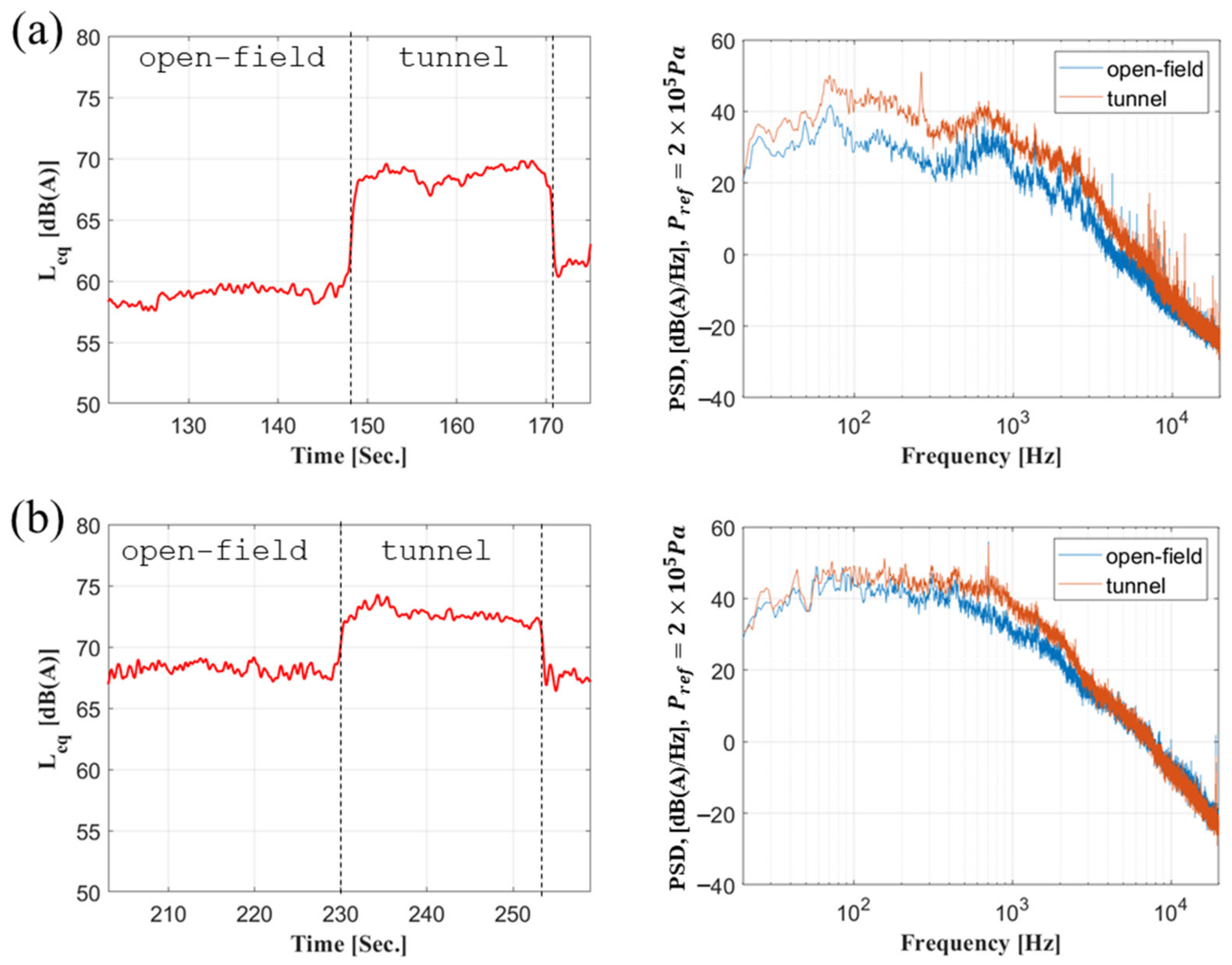
Figure 1. Interior noise (equivalent sound (left) level and PSD level (right)) of two high-speed trains running in open-field and tunnel: (a) KTX and (b) HEMU-430X.
Applsci 11 11702 g001
Figure 2. Illustrative slanted Dirac cone separating incompressible and compressible parts in the three-dimensional periodogram: U 0 = 300 km/h and c 0 = 343 m/s.
Applsci 11 11702 g002
Figure 3. (a) Target train of EMU320 and (b) its detailed parts modeled.
Applsci 11 11702 g003
Figure 4. Computational domain and boundary conditions: (a) open-field case; (b) tunnel case.
Applsci 11 11702 g004
Figure 5. Computational gird descriptions: (a) surface meshes of its main parts, (b) volume meshes of open-field case in x-z plane and (c) volume meshes of tunnel case in the x-y plane.
Applsci 11 11702 g005
Figure 6. Snap-shot of iso-contours of flow velocity magnitude for a train (a) in open-field at t = 1.12 s and (b) in tunnel at t = 1.22 s.
Applsci 11 11702 g006
Figure 7. Snap-shot of iso-contours of static gauge pressure for a train (a) in open field at t = 1.12 s and (b) in tunnel at t = 1.22 s.
Applsci 11 11702 g007
Figure 8. Instantaneous pressure fluctuation contours of (a) open field at t = 1.12 s and (b) tunnel cases at t = 1.22 s.
Applsci 11 11702 g008
Figure 9. Distributions of time-averaged pressure coefficient of open-field case along a line on the train surface at (a) y = 0 m (b) z = 1.017 m.
Applsci 11 11702 g009
Figure 10. Distributions of time-averaged pressure coefficient of tunnel case along a line on the train surface at (a) y = 0 m (b) z = 1.017 m.
Applsci 11 11702 g010
Figure 11. Bogie models used in computations: (a) TC-bogie, and (b) MC-bogie.
Applsci 11 11702 g011
Figure 12. PSD of pressure monitored at probe location (red-dot) at centered vertical plane of y = 0.
Applsci 11 11702 g012
Figure 13. (a) Iso-contours of instantaneous vorticity magnitude in first bogie cavity and (b) snapshot of instantaneous pressure fluctuations around train head in x-z plane of y = 0 with amplitude variation for train in open-field at t = 1.12 s.
Applsci 11 11702 g013
Figure 14. Pantograph and Roof fairing models: (a) on M1-car; (b) on M’3-car.
Applsci 11 11702 g014
Figure 15. Snap-shot of vorticity magnitude contours on the x-z plane at y = 0 m for the train in open-field at t = 1.12 s: (a) first pantograph; (b) second pantograph.
Applsci 11 11702 g015
Figure 16. Characterization of aerodynamic noise generation due to flow around pantograph: (a) PSD levels of pressure monitored at probe location (red-dot) on contact strip of second pantograph, and (b) instantaneous filtered pressure fluctuations of 197.2 Hz at t = 1.12 s.
Applsci 11 11702 g016
Figure 17. Characterization of aerodynamic noise generation due to flow around HVAC box: (a) PSD levels of pressure monitored at probe location (red-dot) on HVAC box of head roof, and (b) instantaneous filtered pressure fluctuation of 128.6 Hz at t = 1.12 s.
Applsci 11 11702 g017
Figure 18. Surface region (Plane-A) of TC-car selected for wavenumber-frequency analysis.
Applsci 11 11702 g018
Figure 19. Three-dimensional PSD diagram (left) and two-dimensional diagram at k x 2 = 0 for plane-A of TC-car (reference pressure 20 μPa).
Applsci 11 11702 g019
Figure 20. Decomposition of surface pressure field into compressible and incompressible pressure: (a) PSD levels of total, compressible, and incompressible pressure parts (reference pressure 20 μPa), and (b) decomposed instantaneous surface gauge pressure of incompressible (left) and compressible (right) field in time-space domain.
Applsci 11 11702 g020
Figure 21. Surface regions selected for wavenumber-frequency analysis: Planes of (a) B and (b) C.
Applsci 11 11702 g021
Figure 22. Two-dimensional diagram at k x 2 = 0 (left) and PSD levels of total, compressible, and incompressible pressure fields (right): (a) Plane-B and (b) Plane-C.
Applsci 11 11702 g022
Figure 23. Overall PSD levels of each surface regions of the open-field case: (a) undecomposed, (b) incompressible and (c) compressible pressure fluctuations.
Applsci 11 11702 g023
Figure 24. Overall PSD levels of each surface regions of the tunnel case: (a) undecomposed, (b) incompressible and (c) compressible pressure fluctuations.
Applsci 11 11702 g024
Figure 25. Overall PSD levels of each surface region along the x-direction of the open-field and tunnel cases.
Applsci 11 11702 g025
Table 1. Related running conditions of three high-speed trains and overall levels.
VehicleRunning ConditionsRunning Speed [km/h]Noise Level [dB(A)]
KTXOpen-field18759.3
Tunnel21768.1
HEMU-430XOpen-field19268.5
Tunnel20572.9
Table 2. Discretization schemes of governing equations.
EquationsDiscretization Method
PressureSecond order
MomentumBounded central differencing
EnergySecond-order upwind
Transient formulationSecond-order implicit
Table 3. Details on boundary setting for open field(O) and tunnel(T) cases.
CaseBoundary TypeSettingRemarks
O/TInlet boundaryVelocity inlet83.33 m/s, non-reflecting
O/TOutlet boundaryPressure outlet101,325 Pa, non-reflecting
O/Side and upper boundaryPressure far field101,325 Pa, Ma = 0.24
/TTunnel wallMoving wall83.33 m/s
O/TGroundMoving wall83.33 m/s
O/TEMU surfacesNo-slip wall
O/TRailMoving wall83.33 m/s
Publisher’s Note: MDPI stays neutral with regard to jurisdictional claims in published maps and institutional affiliations.

