Development of Dynamics for Design Procedure of Novel Grating Tiling Device with Experimental Validation

Abstract

The article proposes a dynamic for design (DFD) procedure for a novel aperture grating tiling device using the multibody system (MBS) approach. The grating device is considered as a rigid-flexible MBS that is built primarily based totally at the load assumptions because of grating movement. This movement is utilized in many industrial applications, such as the compression of laser pulse, precision measuring instruments, and optical communication. A new design procedure of tiling grating device frame is introduced in order to optimize its design parameters and enhance the system stability. The dynamic loads are estimated based on the Lagrange multipliers that are obtained from the solution of the MBS model. This model is fully non-linear and moves in the three-dimensional space, and the relative movement of its bodies is restricted by the description of the constraints function in the motion manifold. The mechanism of the grating device is structurally analyzed in keeping with the dynamic conduct and therefore the generated forces. The symbolic manipulation as well as the computational work of solving the obtained differential-algebraic equations (DAEs) is carried out using MATLAB Symbolic Toolbox. Once the preliminary design has been attained, the stress behavior of the grating device is examined using the MATLAB FEATool Multiphysics toolkit, regarding system stability and design aspects. Moreover, the design was constructed in real life, and the movement has been verified experimentally, which confirms the effectiveness of the proposed procedure. In conclusion, the DFD procedure with trade-off optimization is utilized successfully to design the grating unit for maximum ranges of grating movements.

1. Introduction

The increasing need for high inertia and ultra-precision in optical devices of observational instruments motivates researchers to develop new design of grating tiling device [1]. The research activities on grating device have newly gained greater attention for industrial applications as their advantages become better known and undoubtedly documented [2]. The kinematic and dynamic analysis of the grating device are the most paramount parameters used in optimizing the grating device design [3]. The stability of tiling grating device is one of the most important parameters which need to be achieved. The main factors affecting the stability of grating mechanism are environmental vibration and thermal loading. Grating device stability can be optimized by structural and control algorithm adjustments which are composed of capacitive sensors and piezoelectric ceramic (PZT) actuator [4].

In previous works, modelling and design of the grating devices was carried out using finite element analysis (FEA) [5,6]. However, FEA always comes at the expense of the increased computational effort and is limited by the computing capabilities. Moreover, the grating devices exhibit definite rigid body motion as well as elastic deformations that might be considered relatively small according to the device movement. Thus, it was pointed out in reference [7] that the multibody dynamics approach may actually be the most suitable for modeling the system.

The goal of the DFD procedure is to obtain an efficient design cycle by integrating the dynamics of interconnected systems, including nonlinearities, vibration analysis and parameters estimation, with current design methodologies [8,9]. In the last two decades, MBS became the most effective tool in modeling complex mechanical systems for simulation and system analysis. Many commercial and educational programs have adopted the MBS approach to develop systematized subroutines to build the dynamic structure of systems [10].

In contrast to the finite element method, the MBS approach is the best-suited for modeling dynamic systems that exhibit rigid body motion with definite rotation as well as small and/or large deformation [11,12]. Three formulations for modeling dynamic problems associated with flexible multibody system approach are found in literature, which include the floating frame of reference (FFR) [13], and the structure-preserving method [14] and the absolute nodal coordinate (ANC) method [15]. In view of the nature of the movement in the grating system application under study and its motion characteristic that is associated with limited deformation, the (FFR) formula was used in this work.

In this paper, firstly, the grating system is described, the multibody model is introduced and the resulting terms of equations of motion are constructed using MATLAB Symbolic Math Toolbox. Second, the proposed DFD procedure is utilized to optimize the design of the grating device system. Finally, the designed grating system device is manufactured, assembled and exploited for experimental validation. The remainder of this study is organized as follows: Section 2 describes the grating device mechanism as a multibody system. In Section 3, the system equations of motion are derived and presented, and the mathematical model is constructed. Section 4 presents the numerical results and discussion that are followed by the experimental validation in Section 5, and the conclusion is listed in Section 6.

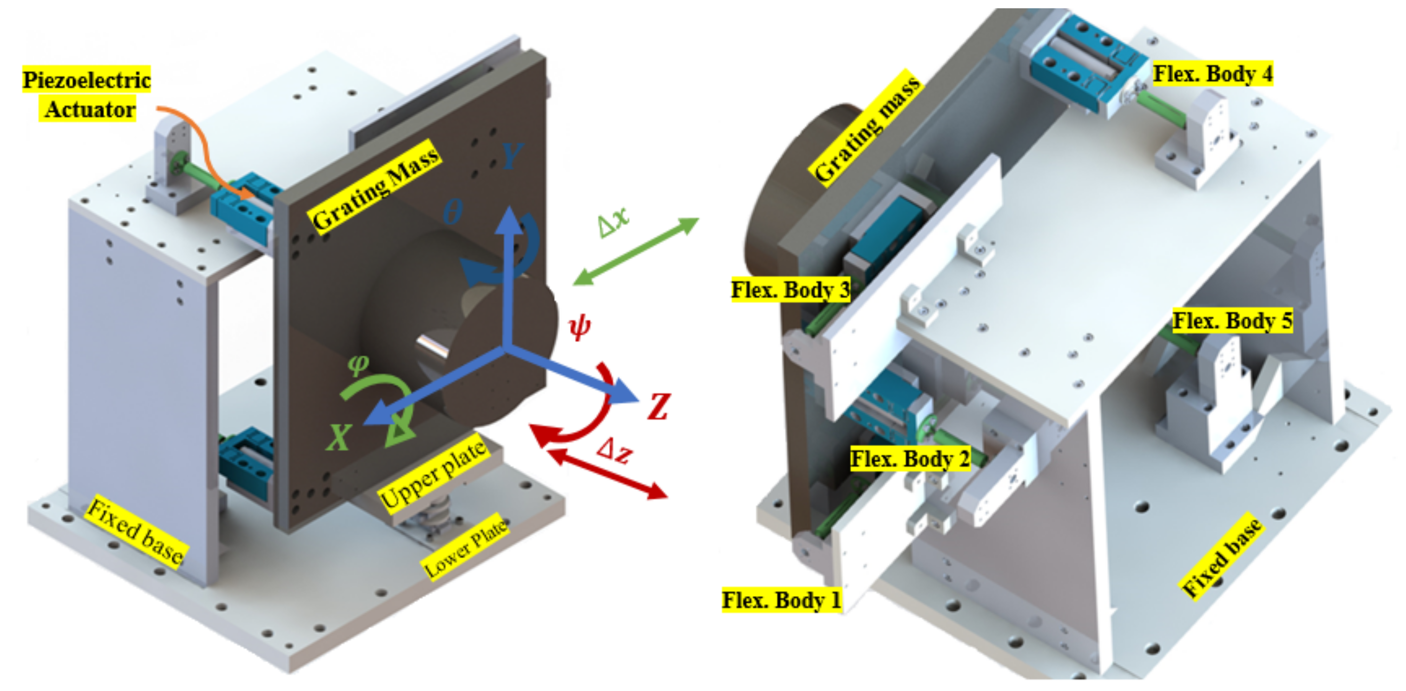
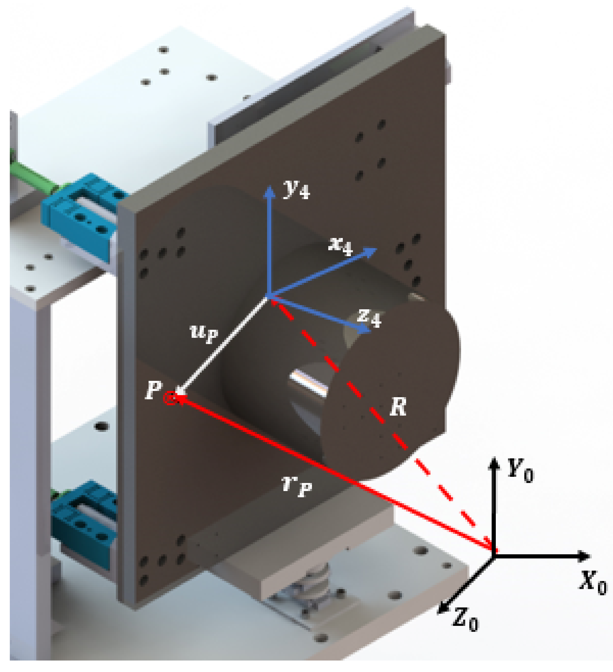
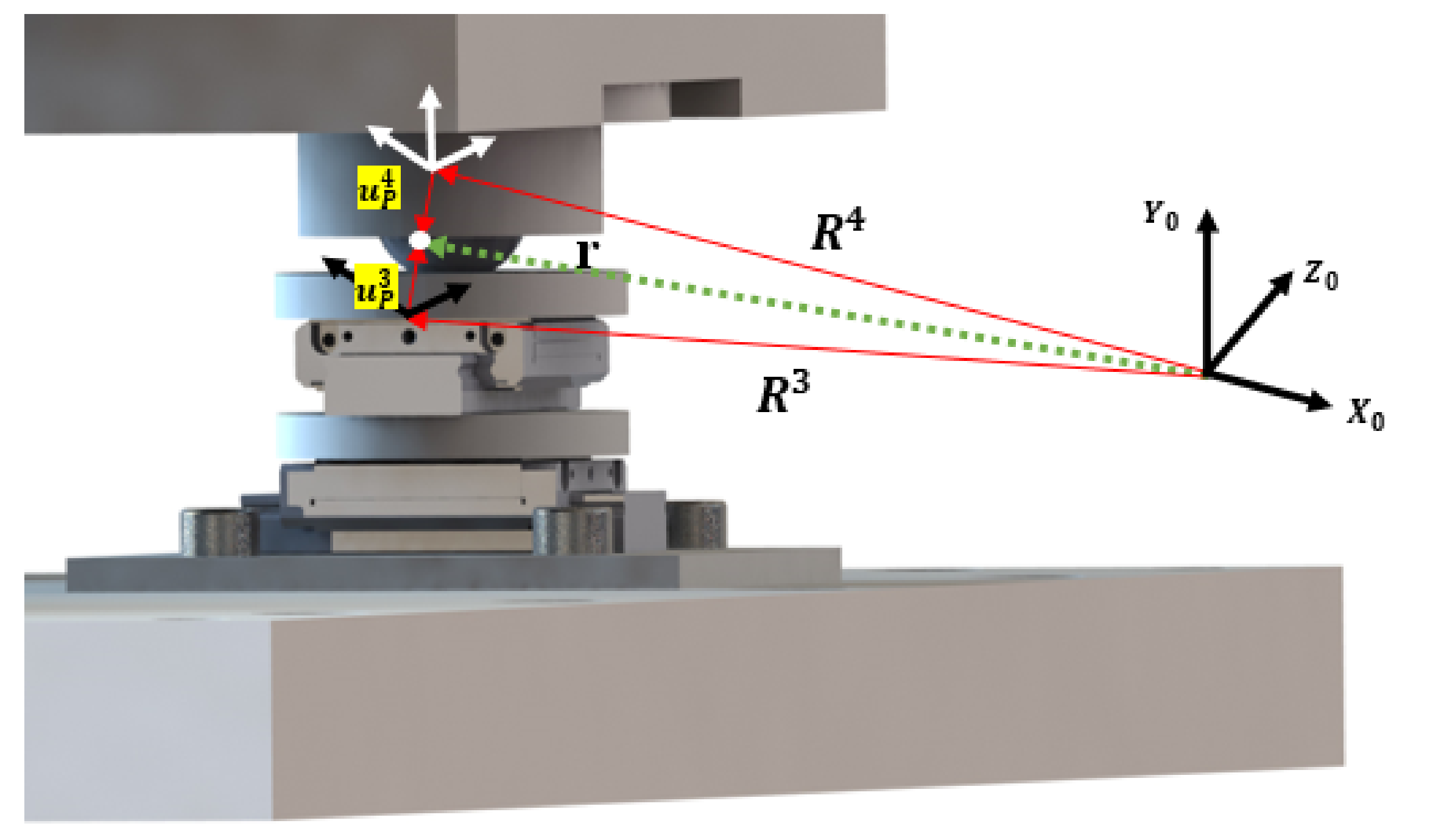
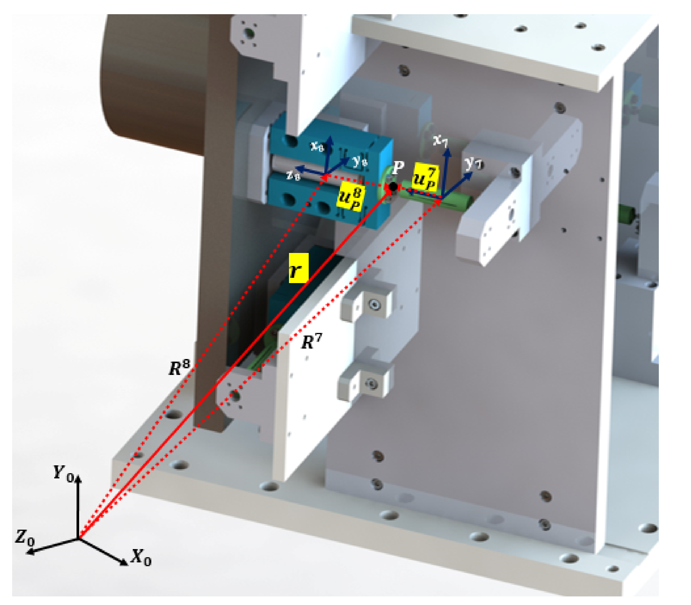
2. Kinematics of Grating Device as a Multibody System

2.1. Kinematics Grating Device

The grating device can be recognized as a typical parallel mechanism [16]. A floating mass, called grating mass, is fixed with five piezo actuators in order to move it laterally and longitudinally and make three independent rotations along perpendicular axes, see Figure 1. The system consists of fixed base, lower plate, upper plate, grating mass, five flexure structures and five flexible rods. The mechanism includes two prismatic joints and one spherical joint. The spatial movement consisted of five degrees of freedom (DOFs) of macro-micro scale compliant parallel mechanism. Specifically, the five movements include two translational DOFs along the X and Z axes of the grating frame and with three rotational degrees about the local axes [17].

The generalized coordinates of each body consist of three translational and four rotational coordinates. The complete generalized coordinates vector can be assembled by embedding vertically the individual coordinates of each body. Defining an arbitrary point P located on the grating mass, see Figure 2, the global position, $\mathbf{r},$ can be expressed as:

$${\mathbf{r}}_p^i={\mathbf{R}}^i+{\mathbf{u}}_p^i={\mathbf{R}}^i+{\mathbf{A}}^i({\overline{\mathbf{u}}}_r^i+{\overline{\mathbf{u}}}_f^i)$$

(1)

where ${\mathbf{r}}_p^i={[r_x^i,r_y^i,r_z^i]}^T$, $i=4$, is the global position vector of point P with respect to global frame which is fixed. ${\mathbf{R}}^i={[R_x^i,R_y^i,R_z^i]}^T$ is the global position vector of frame of the grating mass with respect to global frame, ${\mathbf{A}}^i$ is the transformation matrix between the global and local frames, such that ${\mathbf{u}}_p^i={\mathbf{A}}^i{\overline{\mathbf{u}}}_p^i$ where ${\overline{\mathbf{u}}}_p^i$ is the local position vector of P with respect to the local frame of the grating mass. Actually ${\overline{\mathbf{u}}}_p^i$ equal the combination of ${\overline{\mathbf{u}}}_r^i$ for rigid body motion and ${\overline{\mathbf{u}}}_f^i$ for elastic deformation. Equation (1) illustrates that the position vector of point P can be written as a function in the rotational coordinates, ${\theta }^i={[{\varphi }^i,{\theta }^i,{\psi }^i]}^T$ and translation coordinates, ${\mathbf{R}}^i$. In this paper, three successive rotations about $ZXZ$ are used to describe the orientation of the grating device, they are referred to as Euler angles representation [18].

2.2. System of Equations of Motion

In the floating frame of reference formulation, the flexible body’s deformation can be defined with respect to its reference [19]. The constraints equation of MBS with rigid and flexible bodies can be written as: ]

$$\mathbf{C}({\mathbf{q}}_r,{\mathbf{q}}_f,\mathbf{t})=\mathbf{0}$$

(2)

where $\mathbf{C}$ is constraint functions vectors, ${\mathbf{q}}_r$ is rigid bodies coordinates vector, ${\mathbf{q}}_f$ is flexible bodies coordinates vector and $\mathbf{t}$ is vector of the time. The MBS equations of motion can be written as [20]:

$$\left[\begin{array}{ccc}{\mathbf{M}}_{rr}& {\mathbf{M}}_{rf}& {\mathbf{C}}_{q_r}^T\\ {\mathbf{M}}_{fr}& {\mathbf{M}}_{ff}& {\mathbf{C}}_{q_f}^T\\ {\mathbf{C}}_{q_r}& {\mathbf{C}}_{q_f}& \mathbf{0}\end{array}\right]\left[\begin{array}{c}{\ddot{\mathbf{q}}}_{\mathbf{r}}\\ {\ddot{\mathbf{q}}}_{\mathbf{f}}\\ \lambda \end{array}\right]=\left[\begin{array}{c}{\mathbf{Q}}_r\\ {\mathbf{Q}}_f\\ {\mathbf{Q}}_d\end{array}\right]$$

(3)

where ${\mathbf{M}}_{\mathbf{rr}}$ and ${\mathbf{M}}_{\mathbf{ff}}$ is the system mass matrix related to rigid bodies and flexible bodies, respectively. The dynamic coupling among the rigid body movement and the flexible body deformation is described by the matrix ${\mathbf{M}}_{\mathbf{rf}}$ and the matrix ${\mathbf{M}}_{\mathbf{fr}}$. The matrices ${\mathbf{C}}_{\mathbf{q}r}$ and ${\mathbf{C}}_{\mathbf{q}f}$ are the Jacobian matrices, $\lambda$ is the Lagrange multipliers vector, ${\mathbf{Q}}_r={\mathbf{Q}}_{ex}$ is the external applied forces vector acting on rigid bodies, ${\mathbf{Q}}_f$ is the external applied forces vector acting on flexible bodies and ${\mathbf{Q}}_d$ is the quadratic velocity vector. The constraints Jacobian matrix plays the most important role in kinematic and dynamic analyses of a multibody system. In the case of linear kinematic constraints, the contribution to this matrix can be constant in the coordinates [21].

Equation (3) yields a system of DAEs. The solution obtained the acceleration vector $\ddot{\mathbf{q}}$ and Lagrange multipliers $\lambda$. The acceleration vector can be integrated forward to compute system velocities and configurations. The Lagrange multipliers vector is used for calculating the generalized reaction forces that are used for establishing the design stage [22]. Because of the direct numerical solution DAEs associated with the constrained dynamics of a multibody system poses several computational difficulties mainly related to stability [23]. A post-stabilization approach is employed to bring the position and velocity back to the invariant manifold [24]. Position stabilization and velocities stabilization were done for the modeling system. Following the Lagrange multiplier method, the numerical algorithm of the equations of motion may proceed as follows:

• An estimate of the preliminary situations that outline the preliminary configuration of the multibody model is formed. The preliminary situations that constitute the preliminary coordinates and velocities should be an excellent approximation of the precise preliminary configuration:
• Using the preliminary coordinates, the constraint Jacobian matrix is constructed, assemble the global mass matrix and other equation of motion items;
• Solve the linear set of the equations of motion Equation (3) for a constrained multibody system in order to obtain the accelerations at instant time and the Lagrange multipliers;
• Integrate the accelerations determined the coordinates and velocities. The vector of Lagrange multipliers can be used to determine the generalized reaction forces using Equation (4);
• This process is maintained until the preferred give up of the simulation time is reached.

2.3. Design of Grating Device

Mechanical design is the process of designing and/or selecting mechanical components and putting them together to accomplish a desired function according to specific needs. Grating device bodies transmit forces from one point to another due to grating movements. These forces produce stresses which are considered as the key factor of design process, in consequence, the relations between allowable materials strength and dimensions of designed components can be formulated. In this paper, the MBS is used to estimate the static and dynamic reaction forces acting on grating device bodies [8].

The flexible and flexure bodies are considering the most important element in the system because they are responsible for grating mass movements. The flexure bodies with a novel design give required stiffness to balance the effect elasticity due to flexible bodies [25]. The purpose of flexible and flexure bodies is to give maximum range of grating movements and it must be designed to have the sufficient dynamic structural stability against the extreme loading and abnormal operation conditions and preventing the structural failure [26].

$$\left[\begin{array}{c}{\mathbf{F}}^i\\ {\mathbf{M}}^i\end{array}\right]=-\left[\begin{array}{c}{\mathbf{C}}_R^{{}^{i}T}\\ {\mathbf{C}}_{\theta }^{{}^{i}T}\end{array}\right]{\lambda }^i$$

(4)

where $\mathbf{F}i$ and ${\mathbf{M}}_i$ are denoted the vectors of reaction forces and torques. ${\mathbf{C}}_R^{{}^{i}T}$ is a Jacobian matrix related to translation coordinates and ${\mathbf{C}}_{\theta }^{{}^{i}T}$ is a Jacobian matrix related to rotational coordinates for rigid and flexible bodies. According to the flowchart shown in Figure 3, the dynamic for design procedure is carried out in several stages. Firstly, the grating device system is drawn in the CAD program to obtain the initial parameters required for analysis. Secondly, the mathematical model is built using a multibody system approach and equations of motion are contracted. By solving the equations of motion, the system bodies accelerations and Lagrange multipliers are obtained. The accelerations are integrated forward to obtain the system velocities and configurations until the end of the simulation time. The reaction forces and torques Equation (4) can obtain from the multibody model using Lagrange multipliers. The stress behavior of the grating device is examined using the MATLAB FEATool Multiphysics toolkit based on reaction forces obtained from the multibody model and selected suitable materials for system components. Finally, the optimum design is achieved by changing materials of flexible and flexure bodies and the system dimensions until reaching the maximum range of grating movement parameters.

3. Multibody Model of Grating Device

The grating device system model shown in Figure 1 can be constructed without loss of generality, as shown in

Table 1. Grating device bodies.

Joint Type	Body(i)	Body(j)
Fixed	Grating Base	Ground
Prismatic(Z)	Lower plate	Grating Base
Prismatic(X)	Upper plate	Lower plate
Spherical	Grating mass	Upper plate
Fixed	Flexure bodies	Grating mass
Fixed	Flexible bodies	Flexure bodies
Fixed	Flexible bodies	Grating base

. According to the application, the grating mass motion can be described with five DOFs: translation X and Z and rotational $\varphi$, $\theta$ and $\psi$.

The grating mass can be defined with respect to generalized coordinate as:

$${\mathbf{q}}^i={\left[R_x^i{R}_y^i{R}_z^i{\varphi }^i{\theta }^i{\psi }^i\right]}^T$$

(5)

where ${\mathbf{q}}^i$ is body generalized coordinates. The system of generalized coordinates of all grating device bodies can define as:

$$\mathbf{q}={\left[{\mathbf{q}}^1{\mathbf{q}}^2{\mathbf{q}}^3{\mathbf{q}}^4{\mathbf{q}}^5\dots \dots ,{\mathbf{q}}^{14}\right]}^T$$

(6)

Kinematics constraints equations of spherical, prismatic and rigid joints are used to drive constraints equations of grating system. The rigid joint between grating mass and ground can be obtained by constraining all degree of freedom using mathematical equations [27]. The constraints equations of the rigid joint between fixed base and ground can be written as:

$${\mathbf{C}}_{({\mathbf{q}}^1,{\mathbf{q}}^g,t)}^1=\left[\begin{array}{c}{R}_{{}_x}^1\\ R_{{}_y}^1\\ R_{{}_z}^1\\ cos\left({\psi }^1\right)\ast cos\left({\varphi }^1\right)\ast cos\left({\theta }^1\right)-sin\left({\psi }^1\right)\ast sin\left({\varphi }^1\right)\\ cos\left({\varphi }^1\right)\ast sin\left({\psi }^1\right)+cos\left({\psi }^1\right)\ast sin\left({\varphi }^1\right)\\ cos\left({\varphi }^1\right)\ast sin\left({\theta }^1\right)\end{array}\right]=0$$

(7)

where ${\mathbf{q}}^g$ is generalized coordinate vector for ground and it equals zero. The prismatic joint can also be obtained by eliminating the freedom of the relative rotation between the two bodies about the joint axis and the freedom of the relative translation on one axis [28]. A prismatic joint which allows grating mass to translate in Z direction is shown in Figure 4.

Constraints equations of prismatic joints between lower plate and upper plate can be written as:

$${\mathbf{C}}_{({\mathbf{q}}^2,{\mathbf{q}}^3,t)}^3=\left[\begin{array}{c}{\mathbf{h}}^2\times {\mathbf{h}}^3\\ {\mathbf{h}}^2\times {\mathbf{S}}^{23}\\ {\mathbf{n}}^{2T}{\mathbf{n}}^3\end{array}\right]=0$$

(8)

where $h^2$, $h^3$, $n^2$, $n^3$ and $S^{23}$ are orthogonal vectors, see Figure 4. Equation (8) contains five independent constraint equations that define the kinematic conditions for the single-degree-of-freedom prismatic joint. Constraint equations of spherical joint shown in Figure 5 can be written as:

$${\mathbf{C}}^4({\mathbf{q}}^3,{\mathbf{q}}^4,t)={\mathbf{r}}_p^3-{\mathbf{r}}_p^4=\mathbf{0}$$

(9)

$${\mathbf{C}}^4({\mathbf{q}}^3,{\mathbf{q}}^4,t)={\mathbf{R}}^{{}_3}+{\mathbf{A}}^3{\overline{\mathbf{u}}}_3^i-{\mathbf{R}}^4-{\mathbf{A}}^4{\overline{\mathbf{u}}}_p^4=\mathbf{0}$$

(10)

where ${\mathbf{R}}^{{}_3}$ and ${\mathbf{R}}^4$ are the global position vectors of local frames of bodies 3 and 4, respectively. The matrices ${\mathbf{A}}^3$ and ${\mathbf{A}}^4$ are the transformation matrices. Finally, ${\overline{\mathbf{u}}}_p^3$ and ${\overline{\mathbf{u}}}_p^4$ are the local position vectors defined between the body frame and joint frame. As spherical joints only prevent translation movement, Equation (10) can be written as:

$${\mathbf{C}}_{({\mathbf{q}}^3,{\mathbf{q}}^4,t)}^4={\mathbf{R}}^3-{\mathbf{R}}^4=\mathbf{0}$$

(11)

Because spherical joint allowed only rotation about three axes, the constraints equation for spherical joints Equation (11) can be written as a function on translation constraints as:

$${\mathbf{C}}_{({\mathbf{q}}^3,{\mathbf{q}}^4,t)}^4=\left[\begin{array}{c}{R}_{{}_x}^3-R_{{}_x}^4\\ R_{{}_y}^3-R_{{}_y}^4\\ R_{{}_z}^3-R_{{}_z}^4\end{array}\right]=0$$

(12)

In FFR formulation, fixed joints can be modeled similarly as in rigid multibody systems. Figure 6 shows fixed joint between flexible body2 with flexure body2. Symbolic computer procedure can be used to compute all constraints equations.

The system of external force vector acting in different bodies on grating device can be obtained by the following equation.

$${\mathbf{Q}}_{ex}^i=\left[\begin{array}{c}{\mathbf{Q}}_{exR}^i\\ {\mathbf{Q}}_{ex\theta }^i\end{array}\right]$$

(13)

where ${\mathbf{Q}}_{exR}^i$ is external force associated with translation coordinates and ${\mathbf{Q}}_{ex\theta }^i$ external force associated with rotational coordinates. For grating system the only external forces acting is translation force ${\mathbf{Q}}_{exR}^i={\mathbf{F}}^i$ acting on grating mass as the source of motion and the gravity force ${\mathbf{Q}}_{ex\theta }^i=0$. Piezoelectric actuators drive the central axis of the flexible bodies structure and is fixed on the moving grating mass through fluxure bodies. ${\overline{\mathbf{F}}}^i=[{\overline{\mathbf{F}}}_x^i$${\overline{\mathbf{F}}}_y^i$${\overline{\mathbf{F}}}_z^i]$ is force components. The vector ${\mathbf{Q}}_d$ absorbs terms that are quadratic in the velocities $\dot{\mathbf{q}}$ which appearance with differentiating the constraints equation in terms of time to get velocity and acceleration. The quadratic velocity vector can be written as:

$${\mathbf{Q}}_d{=-(\mathbf{C}}_q{\dot{\mathbf{q}})}_q{\dot{\mathbf{q}}-2\mathbf{C}}_{qt}{\dot{\mathbf{q}}-\mathbf{C}}_{tt}$$

(14)

The vector ${\mathbf{C}}_{tt}$ is the vector of second partial derivative of the constraint equations with respect to time and the vector ${\mathbf{C}}_{qt}$ is the vector of partial derivative of the Jacobian matrix time. The solution of Equation (3) presented in the preceding section defines the vectors of acceleration and Lagrange multipliers. Acceleration can be integrated foreword to obtained grating mass displacement. Forces as the source of stresses can be calculated from the multibody system models as a function of generalized coordinates using Lagrange multipliers.

4. Numerical Results and Discussion

In this section, dynamic for design procedure presented in previous sections is used to design small-scale grating device system using MATLAB symbolic toolbox. The system is fully constructed using CAD software with suitable dimensions and bodies masses and inertias are listed in

Table 2. Grating device parameters employed in the numerical simulation.

Components	Mass (kg)	I${}_{\mathit{x}\mathit{x}}$(kg.m${}^2)$	I${}_{\mathit{y}\mathit{y}}$(kg.m${}^2)$	I${}_{\mathit{z}\mathit{z}}$(kg.m${}^2)$
Grating base	86.34	4.92	3.64	2.8
Disk${}_1$	0.15	0.000035	0.000035	0.000018
Disk${}_2$	0.11	0.000024	0.000013	0.000013
Grating mass	78.26	1.8	1.3	0.985
Flexure part	0.068	0.0001	0.0001	0.0000025
Flexible part	0.012	0.00001	0.00001	0.00000063

and used as initial simulation parameters. The external applied forces due to ceramic piezoelectric actuators are F = 4700 N. By applying external forces, the corresponding frame displacement of the system is obtained by dominant movements of piezoelectric actuators. Figure 7 shows constraints violation due to the prismatic joint between lower plate and grating base. The violation does not exceed $2\times {10}^{-12}$ which indicates the computational efficiency of multibody system model.

Table 3. Displacement range of grating parameters.

DOF	X ($\mathsf{\mu }$m)	Z ($\mathsf{\mu }$m)	$\mathit{\varphi }$ ($\mathsf{\mu }$rad)	$\mathit{\theta }$ ($\mathsf{\mu }$rad)	$\mathit{\psi }$ ($\mathsf{\mu }$rad)
Displacement	±1.5	±3.00	±2.5	±1.5	±2.5

illustrates the degree of freedom movement that the system are able to do.

Figure 8 shows the global position vector of the point $\mathbf{P}$ associated with translation coordinate. The translation along the Z-axis about 3 $\mathsf{\mu }$m in case of applying four forces at flexible bodies 1, 3, 4 and 5. The translation along the X-axis reaches 0.5 $\mathsf{\mu }$m at the same forces while there is no movement along Y-axis which indicates the accuracy of the formulation of multibody constraints.

Figure 9 shows the orientational coordinate of the grating mass with the same applying fores. The grating mass can rotate 2.5 $\mathsf{\mu }$rad about X and Z axis.

In order to optimize the grating device design, a multibody model provides all reaction forces acting on system components with maximum load condition. Figure 10 shows reactions forces acting on grating base, the values of the forces in X-axis and Z-axis are altered and the only reaction force in Y-axis due to the system weight.

Another useful type of data from multibody constraints are reaction moments. Figure 11 shows reactions moments acting on grating base. Likewise, other system bodies’ reaction forces can be computed.

The flexure and flexible bodies should be considered in the design of the tiling system because its the most important factors for system stability. Flexible bodies are an elastic element for the movement of system degree of freedom. The vector of acceleration and Lagrange multipliers associated with flexible bodies can be computed from the multibody model. The acceleration vector is integrated forward in order to calculate elastic displacement of flexible bodies. Figure 12 and Figure 13 shows displacement and orientation of local frame at the middle of the flexible body four due to generalized coordinates associated with flexible bodies.

Similar to rigid body, Lagrange multipliers can be used to compute reaction forces acting on flexible bodies. Figure 14 and Figure 15 shows the reaction forces between flexible and grating base used in design processes.

The material selection as well as the geometrical dimension of flexible and flexure bodies should be estimated to ensure the system’s stability. Therefore, the stiffness of the flexible bodies must be much lower than the rest of the system components with considerable factor of safety.

Table 4. Flexible and Flexure bodies mass properties.

Properties/Body	Flexible	Flexure
Mass (Kg)	0.012	0.068
Density (Kg/m${}^2$)	8000	2810
Elastic Modulus (GN/m${}^2$)	193	72
Poisson ratio	0.27	0.33
Tensile strength (MN/m${}^2$)	5800	2200
Yield strength (MN/m${}^2$)	1720	950

illustrates the primarily design properties of flexible and flexure bodies.

Dynamic reactions forces acting on flexible and flexure bodies are obtained and fed forward to FEATool Multiphysics to examine the stresses with maximum range of grating movement. According to the DFD procedures shown in Figure 3, the stress distribution of flexible body2 with the corresponding displacement along Z-axis show the highest of 1.5 $\mathsf{\mu }$m, see Figure 16 and Figure 17. It is found that, the maximum stress value at the neck point is 700 MN/m${}^2$ which is lesser than yield strength of flexible body material, see Table 4. In addition, the maximum value of the stress on the flexure bodies is less than its material yield strength with factor of safety 3.4. At the end of the procedures, the designed parameters of grating device reach the required performance without breakdown.

5. Experimental Validation

In this section, we describe experimental work carried out to validate the DFD procedures of the designed grating device system, a test system of the grating device as shown in Figure 18 was built and the grating mass movements were measured. The grating device parts are manufactured based on CAD model dimension and selected materials in Table 2 and assembled with other equipment. The equipment includes a piezoelectric actuator with a controller and a displacement sensor with a controller. The piezoelectric actuator used in the grating device test rig is a ceramic type that has a mechanical design of stacked piezoelectric ceramics, combined with a flexible hinge support structure and a shell structure into an integrated structure to form a packaged used in a variety of precision motion control applications. Piezoelectric ceramic actuators have fast response, large generation pressure, and highly accurate operation resonance making it possible to have high micro-displacement resolution and strong stability. The PTZ used in our test has displacement up to 60 $\mathsf{\mu }$m and output force output up to 4700 N with a customized fixed installation structure. The piezoelectric ceramic drive controller is used to control the piezoelectric actuator positions and included a power amplifier, sensor control, chassis and power supply. The high-resolution capacitive displacement sensor system is used to measure the displacements of the grating mass body. Capacitive sensors are designed for non-contact measurement of displacement, distance and position due to their high signal stability and resolution. Capacitive sensors can measure the nano-position of moving objects with excellent precision and duo to the high sensor bandwidth, they can be used in closed-loop control of high dynamics applications. The capacitive non-contact sensor is fully controlled using a servo controller module with a signal amplifier and PC interface. Kinematic results from the capacitive sensor are computed and compared with the multibody system model results.

Figure 19 shows the comparisons between the output grating mass displacement of the MBS model and the experimental data. Since the multibody model and experiment data have similar results, the dynamic for design procedure of the grating device system is accurate and can be used later in system identification and design optimization of the grating device system.

6. Conclusions

This paper introduces a dynamic for design DFD procedure of novel grating tiling device for maximum ranges of grating movements based on the multibody system approach.

(1)

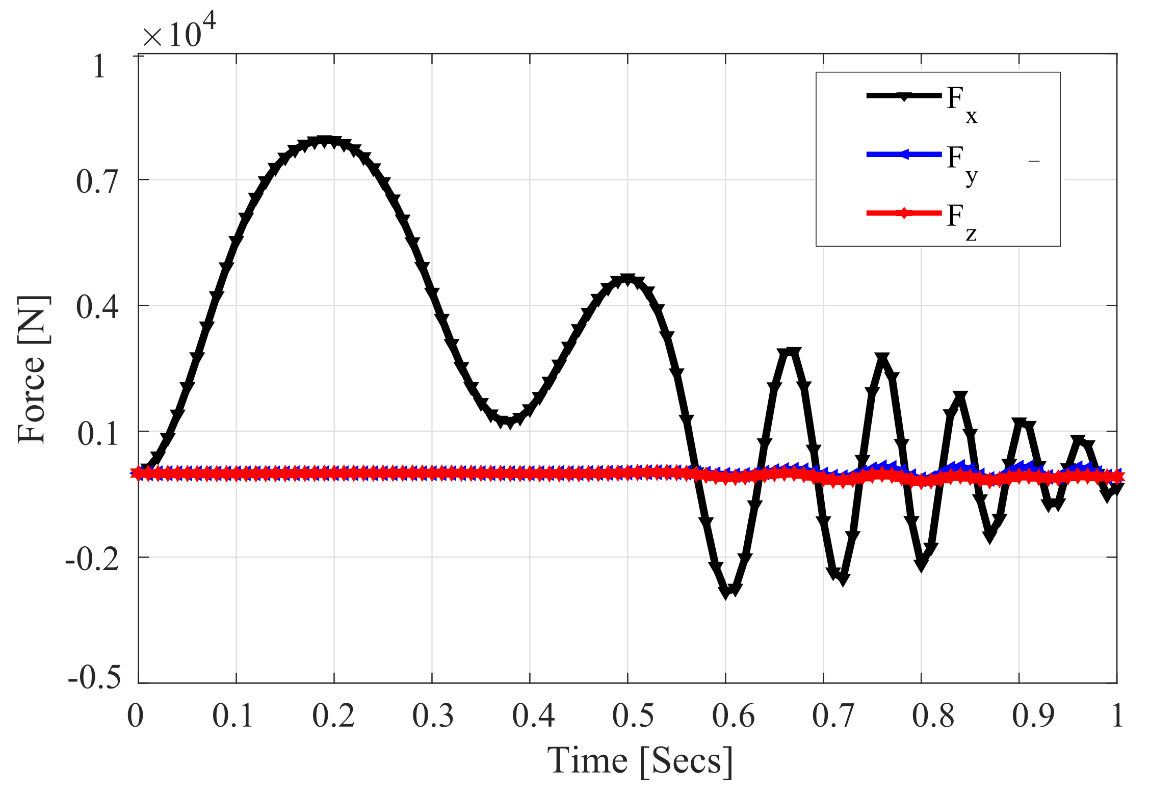
The grating device model was successfully implemented in a simulation tool entirely elaborated in MATLAB including symbolic and computational work. Equation of motion solution included system coordinates and Lagrange multipliers are obtained. These multipliers are used to estimate the reaction forces utilized in the design procedure of the grating system.

(2)

From the results presented in the preceding sections, the optimal design of such a grating device is carried out for maximum ranges of grating movements. The design procedure proposed in this work is systematic and oriented for grating devices to realize the positioning and attitude adjustment of the moving grating.

(3)

The design was constructed in real life and the movement was verified experimentally, which confirms the effectiveness of the proposed procedure. The design method of the grating device system based on the DFD procedure proposed in this paper provides new ideas and methods for the design of large load, and high-precision grating systems.

References

1. Shao, Z.X.; Zhang, Q.C.; Bai, Q.S.; FU, H.Y. Design method of controlling device for tiling high precision and large aperture grating. Opt. Precis. Eng. 2009, 1, 158–165. [Google Scholar]
2. Wu, J.; Luo, Z.; Zhang, N.; Zhang, Y.; Walker, P.D. Uncertain dynamic analysis for rigid-flexible mechanisms with random geometry and material properties. Mech. Syst. Signal Process. 2017, 85, 487–511. [Google Scholar] [CrossRef] [Green Version]
3. Wang, C.; Zhang, Y.; Qian, J.; Sun, L. Precision analysis of a large aperture tiled-gratings device. In Proceedings of the 2014 IEEE International Conference on Robotics and Biomimetics (ROBIO 2014), Bali, Indonesia, 5–10 December 2014; pp. 1175–1179. [Google Scholar]
4. Yunfei, L.; Yi, Z.; Mingjun, M.; Ke, C. Structural stability of large-size grating tiling device based on dynamic stiffness. J. Softw. Eng. 2015, 9, 287–297. [Google Scholar] [CrossRef]
5. Bai, Q.; Liang, Y.; Cheng, K.; Long, F. Design and analysis of a novel large-aperture grating device and its experimental validation. Proc. Inst. Mech. Eng. Part B J. Eng. Manuf. 2013, 227, 1349–1359. [Google Scholar] [CrossRef]
6. Shao, Z.; Wu, S.; Wu, J.; Fu, H. A novel 5-DOF high-precision compliant parallel mechanism for large-aperture grating tiling. Mech. Sci. 2017, 8, 349–358. [Google Scholar] [CrossRef] [Green Version]
7. Bai, Q.; Shehata, M.; Nada, A. Efficient Modeling Procedure of Novel Grating Tiling Device Using Multibody System Approach. In International Symposium on Multibody Systems and Mechatronics; Springer: Córdoba, Argentina, 12–15 October 2020; pp. 168–176. [Google Scholar]
8. Saleh, M.; Nada, A.; El-Betar, A.; El-Assal, A. Computational Design Scheme for Wind Turbine Drive-Train Based on Lagrange Multipliers. J. Energy 2017, 2017, 16. [Google Scholar] [CrossRef]
9. Wang, Z.; Tian, D.; Shi, L.; Liu, J. Multi-Body Dynamics Modeling and Control for Strapdown Inertially Stabilized Platforms Considering Light Base Support Characteristics. Appl. Sci. 2020, 10, 7175. [Google Scholar] [CrossRef]
10. Nada, A.A.; Bishiri, A.H. Multibody system design based on reference dynamic characteristics: Gyroscopic system paradigm. Mech. Based Des. Struct. Mach. 2021, 1–23. [Google Scholar] [CrossRef]
11. Wasfy, T.M.; Noor, A.K. Computational strategies for flexible multibody systems. Appl. Mech. Rev. 2003, 56, 553–613. [Google Scholar] [CrossRef]
12. Zahariev, E.V. Generalized finite element approach to dynamics modeling of rigid and flexible systems. Mech. Based Des. Struct. Mach. 2006, 34, 81–109. [Google Scholar] [CrossRef]
13. Nada, A.; Hussein, B.; Megahed, S.; Shabana, A. Use of the floating frame of reference formulation in large deformation analysis: Experimental and numerical validation. Proc. Inst. Mech. Eng. Part K J. Multi-Body Dyn. 2010, 224, 45–58. [Google Scholar] [CrossRef]
14. Sharma, H.; Patil, M.; Woolsey, C. A review of structure-preserving numerical methods for engineering applications. Comput. Methods Appl. Mech. Eng. 2020, 366, 113067. [Google Scholar] [CrossRef]
15. Shabana, A.A. Definition of ANCF finite elements. J. Comput. Nonlinear Dyn. 2015, 10, 054506. [Google Scholar] [CrossRef]
16. Si, H.; Guo, Y.B.; Liang, Y.C. Application and Developing Trends of Mechanical Tiling Technology in the Laser Fusion Device. In Key Engineering Materials; Trans Tech Publications Ltd.: Bach, Switzerland, 2014; Volume 621, pp. 57–62. [Google Scholar]
17. Rui, X.; Gu, J.; Zhang, J.; Zhou, Q.; Yang, H. Visualized simulation and design method of mechanical system dynamics based on transfer matrix method for multibody systems. Adv. Mech. Eng. 2017, 9, 1687814017714729. [Google Scholar] [CrossRef] [Green Version]
18. Korkealaakso, P.; Mikkola, A.; Rantalainen, T.; Rouvinen, A. Description of joint constraints in the floating frame of reference formulation. Proc. Inst. Mech. Eng. Part K J. Multi-Body Dyn. 2009, 223, 133–145. [Google Scholar] [CrossRef]
19. Pappalardo, C.M.; Lettieri, A.; Guida, D. Stability analysis of rigid multibody mechanical systems with holonomic and nonholonomic constraints. Arch. Appl. Mech. 2020, 90, 1961–2005. [Google Scholar] [CrossRef]
20. O’Shea, J.J.; Jayakumar, P.; Mechergui, D.; Shabana, A.A.; Wang, L. Reference conditions and substructuring techniques in flexible multibody system dynamics. J. Comput. Nonlinear Dyn. 2018, 13, 041007. [Google Scholar] [CrossRef]
21. El-Ghandour, A.; Foster, C. Coupled finite element and multibody systems dynamics modelling for the investigation of the bridge approach problem. Proc. Inst. Mech. Eng. Part F J. Rail Rapid Transit 2019, 233, 1097–1111. [Google Scholar] [CrossRef]
22. Kim, H.W.; Yoo, W.S. MBD applications in design. Int. J. Non-Linear Mech. 2013, 53, 55–62. [Google Scholar] [CrossRef]
23. Ziegler, P.; Humer, A.; Pechstein, A.; Gerstmayr, J. Generalized component mode synthesis for the spatial motion of flexible bodies with large rotations about one axis. J. Comput. Nonlinear Dyn. 2016, 11, 041018. [Google Scholar] [CrossRef]
24. Sugiyama, H.; Escalona, J.L.; Shabana, A.A. Formulation of three-dimensional joint constraints using the absolute nodal coordinates. Nonlinear Dyn. 2003, 31, 167–195. [Google Scholar] [CrossRef]
25. Yoo, W.S.; Kim, K.N.; Kim, H.W.; Sohn, J.H. Developments of multibody system dynamics: Computer simulations and experiments. Multibody Syst. Dyn. 2007, 18, 35–58. [Google Scholar] [CrossRef]
26. Wallin, M.; Hamed, A.M.; Jayakumar, P.; Gorsich, D.J.; Letherwood, M.D.; Shabana, A.A. Evaluation of the accuracy of the rigid body approach in the prediction of the dynamic stresses of complex multibody systems. Int. J. Veh. Perform. 2016, 2, 140–165. [Google Scholar] [CrossRef]
27. Elshami, M.; Shehata, M.; Bai, Q.; Zhao, X. Multibody Dynamics Modeling of Delta Robot with Experimental Validation. In International Symposium on Multibody Systems and Mechatronics; Springer: Córdoba, Argentina, 12–15 October 2021; pp. 94–102. [Google Scholar]
28. Bauchau, O. On the modeling of prismatic joints in flexible multi-body systems. Comput. Methods Appl. Mech. Eng. 2000, 181, 87–105. [Google Scholar] [CrossRef]
Figure 1. Grating device system unit.
Applsci 11 11716 g001
Figure 2. Displacement field of an arbitrary point.
Applsci 11 11716 g002
Figure 3. Dynamic for design procedure for grating tiling device.
Applsci 11 11716 g003
Figure 4. Prismatic joint between base and lower plate.
Applsci 11 11716 g004
Figure 5. Spherical joint between upper plate and grating mass.
Applsci 11 11716 g005
Figure 6. Fixed joint between flexible body2 and flexure body2.
Applsci 11 11716 g006
Figure 7. Constraints violation of the prismatic joint.
Applsci 11 11716 g007
Figure 8. Grating mass displacement.
Applsci 11 11716 g008
Figure 9. Orientation of grating mass around three axes.
Applsci 11 11716 g009
Figure 10. Reaction forces acting on grating base.
Applsci 11 11716 g010
Figure 11. Reaction moments acting on grating base.
Applsci 11 11716 g011
Figure 12. Flexible body 2 elastic displacement.
Applsci 11 11716 g012
Figure 13. Flexible body 2 elastic orientation.
Applsci 11 11716 g013
Figure 14. Reaction forces at fixed joint between flexure and flexible body 2.
Applsci 11 11716 g014
Figure 15. Reaction moments at fixed joint between flexure and flexible body 2.
Applsci 11 11716 g015
Figure 16. Stress distribution on flexible body2.
Applsci 11 11716 g016
Figure 17. Flexible body2 displacement along the Z-axis.
Applsci 11 11716 g017
Figure 18. Test rig: (1) grating device, (2) piezoelectric ceramic actuators, (3) piezoelectric actuators controller, (4) capacitive displacement sensor, (5) displacement sensor controller, (6) display computer.
Applsci 11 11716 g018
Figure 19. Comparison between MBS model result and experimental data.
Applsci 11 11716 g019