The Role of Buoyancy Induced Instability in Transpirational Cooling Applications

Abstract

Transpirational cooling is an effective thermal protection method in hypersonic vehicles. In order to properly manage the high heat load, an understanding of the convective flow regimes as well as the thermophysical properties of the working fluid are required. Often, the vehicle’s fuel is re-purposed as the coolant or working fluid that is passed through the porous media. If the geometry is such that the coolant is heated from below, buoyancy-induced instability can ensue resulting in a mixed convection phenomena. Transpirational cooling applications require a unique analysis which combines a Darcy–Forchheimer relationship for the momentum relation, a flowing base state which introduces non-negligible convective terms for the energy equation, and a novel consideration of a cubic density dependence on temperature. This latter feature is justified by fitting thermodynamic data for typical transpirational cooling conditions. A base state solution is provided and the onset of instability is investigated using linear stability analysis. The governing equations are solved utilizing multiple methods, comparing results from a combination of analytical solutions, finite difference, power series, and Chebyshev methods. Results demonstrate excellent consistency in predictions across these methods and indicate that including non-linear density effects promote a stabilizing effect. Finally, the effect of varying the net through-flow in the porous media is investigated.

1. Introduction

Transpirational cooling is an effective thermal protection method in hypersonic vehicles. The transpirational cooling concept was first applied to the throat of rocket engines in the 1940s. Since then it has been applied to other parts of the aircraft that experience high heat loads such as the leading edge and fuel injection strut. Often, the vehicle’s fuel is re-purposed as the coolant or working fluid that is passed through a porous media section to form a continuous thin film over the protected wall. Thus, a proper understanding of the underlying mechanisms in transpirational cooling applications leads to more robust design capable of handling higher heat loads.

Early investigation of transiprational cooling phenomena was carried out by Rannie [1] who analytically modeled the porous wall temperature to investigate the laminar transpired sublayer. His model aligned with experimental data at low thermal conductivity for the porous substrates. Other analytical approaches for transpirational cooling have also been detailed by Eckert [2,3] including how to model coolant injection and hot gas heat transfer from an exterior hot boundary layer. Recently, a closed form analytical solution was developed for 2D pressure and velocity field for transpirational cooling applications [4]. Several experimental works have been put forth detailing the effects of the transpirant, mass flow rate, inlet temperature, flow coking, etc. on cooling efficacy and performance [5,6,7,8]. Dahmen et al. [9] analyzed the experimental transpirational cooling setup in Ref. [6], using numerical simulation to provide full flow field details that were difficult to acquire through experiments. Other computational studies have been performed that quantify cooling efficacy versus inlet conditions, thermal properties, and boundary conditions [10,11].

All previous studies have either analytically, experimentally, or numerically, investigated transiprational cooling in geometric configurations where the hot surface is on the top or side and the cold surface is on the bottom or side. However, if the geometry is such that the hot surface and cold surface are on the bottom and top, respectively, then Bénard-type convection can ensue resulting in a mixed convection phenomena. This type of arrangement occurs on the bottom wall of the aircraft or the top wall of the combustion chamber. In these cases, an understanding of the buoyancy-induced instability mechanisms need to be described and understood. The tools of linear stability analysis provide a pathway for this understanding.

A similar geometric and flow configuration to that occurring in transpirational cooling applications, albeit with no base flow, is the Horton–Rogers–Lapwood (HRL) problem. The HRL problem consists of a buoyancy-induced instability in porous media due to heating from below [12,13]. The HRL problem is extensively described and characterized in Nield and Bejan [14]. A pioneering variation of the HRL problem where base flow is perpendicular to the base temperature gradient was studied by Prats [15]. Several variations of the HRL and Prats problems have been investigated by Barletta and Celli [16,17,18]. The variation of the HRL problem most relevant to the transpirational cooling problem at hand is with a base flow parallel in the direction of the base temperature gradient, i.e., vertical base flow. This problem was first studied by Wooding [19] on a semi-infinite (vertical) porous domain. Sutton then characterized stability in a finite domain–of both width and height–against through-flow velocities of a small magnitude [20]. Initially, a small negative through-flow has a slight destabilizing effect which transitions to a stabilizing effect as velocity is increased. This effect is exaggerated as the domain width becomes smaller. Next, Homsy and Sherwood investigated the stability theory on a finite domain for both strong and weak through-flows [21]. They found that mass discharge in the positive vertical direction destabilizes while the opposite was true for negative through-flow.

The previous works provide much insight to buoyancy-induced instabilities occurring in porous media applications such as transpirational cooling. However, transpirational cooling has additional complexities which are not accounted for by the hydrodynamic stability analysis in these works. These include the highly non-linear density variation with temperature, i.e., a nonlinear Boussinesq approximation [22,23]. Due to the often extreme temperature difference between the inlet and exit of the porous media, extremely large density gradients can occur. These density gradients arise from heating cryogenic fuels like methane or hydrogen to a supercritical state. Real-gas compressibility effects can be significant at these extreme temperatures and pressures. Thus, the objective of this work is to include the effects of a non-linear cubic density dependence on temperature in a base state configuration with a vertical through-flow to quantify and understand the instability mechanisms occurring in the porous medium. Three cases are considered in this work, each with an additional layer of complexity: (1) A traditional HRL configuration, (2) a HRL configuration with a non-linear density variation in temperature, and (3) adding a base vertical through-flow to Case 2. The third case is most representative of transpirational cooling. The non-dimensionalization introduced in this study to account for the drag term results in a Grashof-type scaling rather than the typical Rayleigh-type scaling encounter in HRL (or Wooding) style problems. The resulting equations are solved using a power series method, Chebyshev method, and finite difference method. The three cases of increasing complexity elucidate how the various effects of a non-linear density and a varying vertical through-flow affect the stability in transpirational cooling systems.

This work is divided into five sections. First, the mathematical framework used to study transpirational cooling is described. Second, linear stability analysis is performed and detailed. Next, an overview of the various solution techniques are outlined. Finally, results are given followed by a discussion and conclusions.

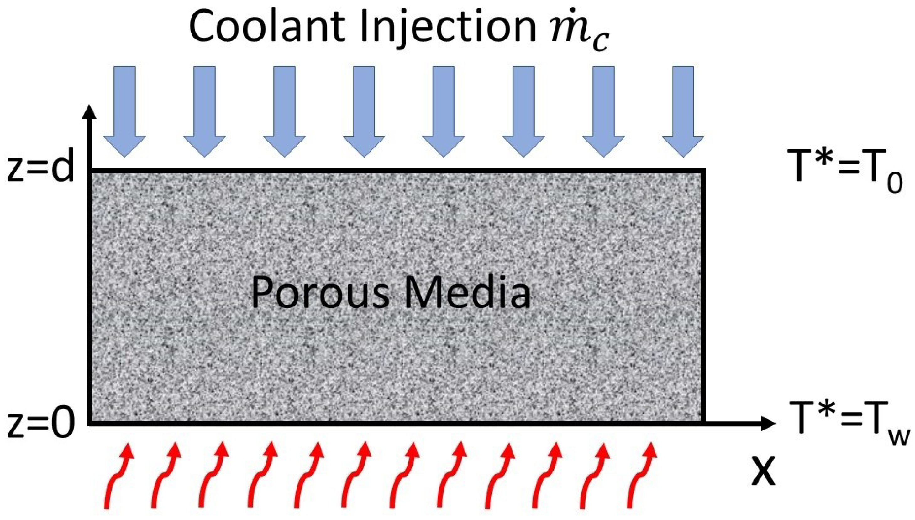
2. Mathematical Model

2.1. Governing Equations

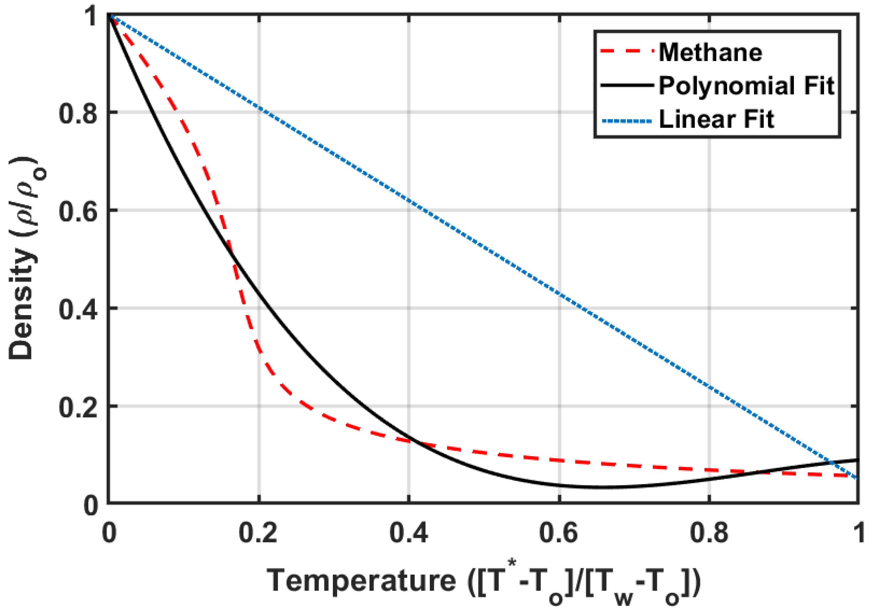
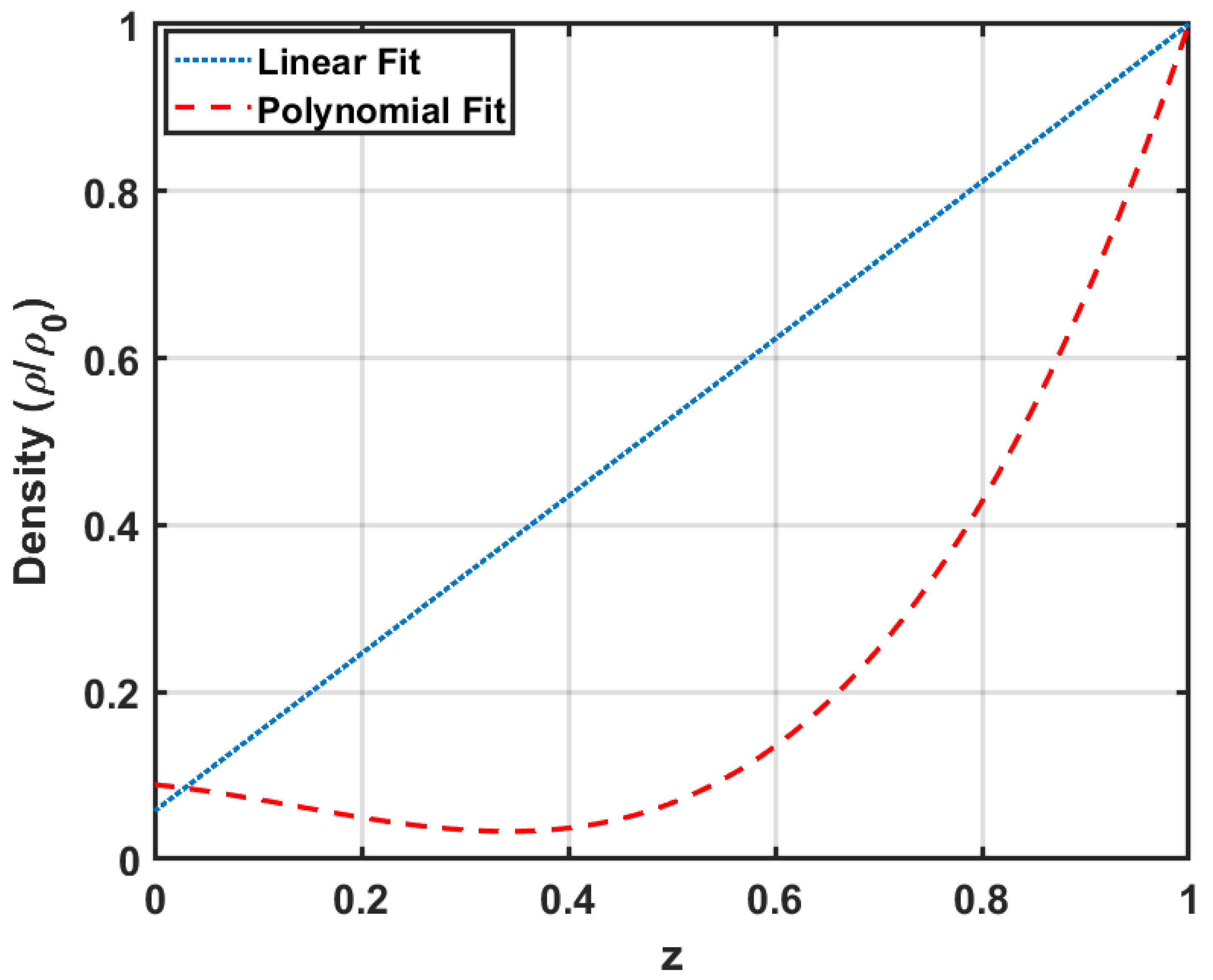
A simplified model for transpirational cooling is presented in Figure 1. Here, a fluid-saturated isotropic porous medium of infinite horizontal extent is confined between two permeable boundaries a distance d apart. The hot gas flowing over bottom layer is modeled as a constant temperature boundary condition as in Ref. [6]. Coolant continuously flows over the top permeable boundary ($z=d$ in Figure 1), and creates an isothermal condition. Wall suction provides a constant coolant injection aligned with the gravitation vector [3]. This following problem configuration is similar to the Wooding problem [19], where a constant through-flow is heated which gives rise to an additional thermally-induced natural convection of the Beńard type. These assumptions, along with the Boussinesq approximation, lead to Dirichlet conditions for velocity and temperature at the top and bottom boundary.

Analysis of this problem requires conservation of the mass, momentum, and energy equations subject to the aforementioned boundary conditions. In regards to the momentum equation, several experimental [6,7] and numerical studies [8,9] have determined that transipirational cooling applications are accurately approximated by the Darcy–Forchheimer equation. The curl of the Darcy–Forchheimer equation is presented here to drop the pressure term. The energy equations for the porous material and the fluid phase can be simplified to one equation if local thermal equilibrium exists between the solid and fluid phases, and there is no net conduction between the phases [14]. The resulting single equation uses an overall heat capacity and thermal conductivity per unit volume of the porous material and fluid denoted by the subscript ‘m’. For example, ${\left(\rho c_p\right)}_m=(1-\psi ){\left(\rho c_p\right)}_s+\psi {\left(\rho c_p\right)}_f$, where $\psi$ is the porosity and the subscripts ‘s’ and ‘f’ refer to the solid and fluid phase, respectively. Langener and Wolfersdorf [6] investigated these assumptions along with negligible work due to pressure, negligible viscous heating, and constant density in the energy equation to study transpirational cooling in scramjet engines and found good agreement with experimental results. Thus, the resulting energy equation is implemented in Equation (1).

The governing equations and boundary conditions are shown in Equation (1).

$$\left\{\begin{array}{cc}\hfill & \nabla ·{\mathbf{u}}^{*}=0\hfill \\ \hfill & \frac{\mu }{K}(\nabla \times {\mathbf{u}}^{*}+\frac{c_F\sqrt{K}}{\nu }\nabla \times ({\mathbf{u}}^{*}|{\mathbf{u}}^{*}\left|\right))=\nabla \times \rho g{\mathbf{e}}_{\mathbf{z}}\hfill \\ \hfill & {\left(\rho c_p\right)}_m\frac{\partial T^{*}}{\partial t^{*}}+{\left(\rho c_p\right)}_f{\mathbf{u}}^{*}·\nabla T^{*}=k_m{\nabla }^2{T}^{*}\hfill \\ \hfill & z^{*}=0:{\mathbf{u}}^{*}=<0,0,-\lambda \frac{Kg\beta \mathrm{\Delta }T}{{\nu }^2}>,T^{*}=T_w\hfill \\ \hfill & z^{*}=d:{\mathbf{u}}^{*}=<0,0,-\lambda \frac{Kg\beta \mathrm{\Delta }T}{{\nu }^2}>,T^{*}=T_0\hfill \end{array}\right.$$

(1)

The filtration velocity vector is represented by the three orthogonal velocity components, u${}^{*}=<u^{*},v^{*},w^{*}>$, corresponding to the Cartesian position vector, x${}^{*}=<x^{*},y^{*},z^{*}>$. The asterisk here refers to the dimensional quantities. The terms $\nu$, K, $c_F$, $\rho$, $|{\mathbf{u}}^{*}|$, and ‘g’ in the Darcy–Forchheimer equation are the kinematic fluid viscosity, permeability of the porous material, dimensionless Darcy-Forchheimer form drag coefficient, fluid density, velocity magnitude, and gravity, respectively. The term e${}_{\mathbf{z}}$ is the unit vector in the z direction. T${}^{*}$, $c_p$, k, $\beta$, and $\lambda$ are the respective temperature, specific heat, thermal conductivity, coefficient of thermal expansion, and a velocity scaling constant. The subscript ‘0’ and ‘w’ refer to the constant quantity at the top and bottom boundary, respectively. Here, all the properties are assumed constant except the density associated with buoyant forces.

In many transpiration cooling applications, the fuel is often repurposed as the coolant. These fuels, e.g., hydrogen, methane, and other heavier alkanes, are delivered as liquids at high pressures at or above the thermodynamic critical point of the fluid. As the fluid is transpired through the porous material, heating occurs which often causes the fluid to become supercritical (if it is not supercritical to begin with) and causes a reduction in the fluid density. Density gradients are highly nonlinear near the thermodynamic critical point and in the supercritical regions. Accordingly, the stability behavior can be significantly different from systems with linear dependencies. In order to capture these nonlinear effects, density is modeled as a third order polynomial, which qualitatively captures the real-fluid behavior of the coolant as illustrated in Figure 2. This is often considered as the nonlinear Boussinesq approximation [22,23]. Figure 2 shows non-dimensional reduced density, ${\rho }_r=\frac{\rho }{{\rho }_c}$, versus non-dimensional reduced temperature, $T_r=\frac{T^{*}}{T_c}$, of methane and hydrogen generated using real-fluid equations of state implemented through REFPROP [24]. The subscript ‘c’ represents the property at the critical point. Figure 2 shows methane and hydrogen for sweep of reduced pressures from $P_r=1$ to $P_r=$ 5 – a typical pressure range for coolant delivery [25]. A least squares fit using a third order polynomial is shown in Figure 2 as the solid black line. Figure 3 shows typical conditions cooling the throat of a rocket engine using methane with an at in inlet temperature of 105 K and a wall temperature of 755 K with the density (red-dashed line), the polynomial curve fit (black solid line), and the linear fit (blue small-dashed line) [25]. The values are also used for the fluid properties in

Table 1. Value of properties used in this work.

Property	${\mathit{w}}_{\mathit{b}}$ *	K	$\mathit{\beta }$	$\mathbf{\Delta }$ T	$\mathit{\nu }$	L	${\mathit{c}}_{\mathit{F}}$
Units	$\frac{\mathrm{m}}{\mathrm{s}}$	$\mathsf{\mu }{\mathrm{m}}^2$	$\frac{1}{\mathrm{mK}}$	K	$\frac{{\mathrm{cm}}^2}{\mathrm{s}}$	mm	-
Value	0.05–0.15	500–1000	1–5	650	0.003	5–10	5–20
Reference	[6]	[6]	current work	[25]	[24]	[6]	[6]

. Equation (2) shows the third order polynomial:

$$\rho ={\rho }_0(1-\beta \mathrm{\Delta }T\left(T+c_1{T}^2+c_2{T}^3\right)$$

(2)

where the non-linear portion can be separated as the function $f\left(T\right)=c_1{T}^2+c_2{T}^3$. In Equation (2), T is the non-dimensional scaling of temperature where $T=\frac{T^{*}-T_0}{\mathrm{\Delta }T}$, $\beta$ is an average coefficient of thermal expansion, and $\mathrm{\Delta }T=T_w-T_0$. It is worth noting that $\beta$ is different for the linear case compared to the non-linear case. As a result, it varies from the linear case, where $\beta =0.00145$ to the non-linear curve fit where ${\beta }_2=0.0057$. To appropriately compare to linear and non-linear cases, a scale factor, $\beta /{\beta }_2=3.97$, must be accounted for in the results and will be discussed in the later sections.

The system of equations in Equation (1) are non-dimensionalized by introducing the following scaling variables:

$$\mathit{x}={\mathit{x}}^{*}/d,\mathit{u}={\mathit{u}}^{*}\frac{{\nu }^2}{Kg\beta \mathrm{\Delta }T},T=\frac{T^{*}-T_0}{\mathrm{\Delta }T},t=t^{*}\frac{Kg\beta \mathrm{\Delta }T}{\nu L}.$$

(3)

The system of equations in Equation (1) are rewritten as:

$$\left\{\begin{array}{cc}\hfill & \nabla ·\mathbf{u}=0\hfill \\ \hfill & \nabla \times \mathbf{u}+\xi \nabla \times \left(\mathbf{u}\right|\mathbf{u}\left|\right)=\nabla \times T{\mathbf{e}}_{\mathbf{z}}+\nabla \times f{\mathbf{e}}_{\mathbf{z}}\hfill \\ \hfill & \frac{\partial T}{\partial t}+\frac{1}{\sigma }\mathbf{u}·\nabla T=\gamma {\nabla }^{2}T\hfill \\ \hfill & z=0:\mathbf{u}=<0,0,-\lambda >,T=1\hfill \\ \hfill & z=1:\mathbf{u}=<0,0,-\lambda >,T=0\hfill \end{array}\right.$$

(4)

where $\sigma =\frac{{\left(\rho c_p\right)}_m}{{\left(\rho c_p\right)}_f}$, $\xi =c_{F}D{a}^{3/2}Gr$, $\gamma =\frac{k_m/{\left(\rho c_p\right)}_m}{DaGr}$, $Da=\frac{K}{L^2}$ is the Darcy number, and $Gr$ = $\frac{g\beta \mathrm{\Delta }T{L}^3}{{\nu }^2}$ is the Grashof number.

2.2. Base State

The basic steady state energy equation subjected to the aforementioned boundary conditions with a constant through-flow given by $w_b=-\lambda$ is given by Equation (5),

$$C\frac{d{T}_b}{dz}=\frac{d{T}_b^2}{d{z}^2}$$

(5)

where $C=\frac{-\lambda }{\sigma \gamma }$ and the subscript ‘b’ denotes the base state. The basic solution promotes a thermal boundary layer of the exponential form given in Equation (6):

$$T_b\left(z\right)=\frac{1-e^{C(1-z)}}{1-e^C}.$$

(6)

This solution is very similar to the one dimensional solution used to model transpirational cooling experimental data given in Ref. [6], which used constant temperatures for both the top and bottom boundary to match experimental conditions. It is worth noting that the non-linearity in the temperature boundary layer is driven by the velocity magnitude, $\lambda$. In the limit of the velocity magnitude approaching zero, the temperature boundary layer becomes linear and approaches the same basic solution described in Ref. [17], where a porous material with a horizontal rather than vertical through-flow undergoes heating at the bottom boundary with a fixed top boundary temperature.

The basic density profile can be solved for by inserting Equation (6) into Equation (2) (shown later in Section 5). Accordingly, non-linearity in the density is caused from two independent sources: (1) The through-flow velocity and its effect on the temperature profile and (2) inherent non-linearity in the equation of state. Together, these effects manifest large density gradients at the top of the domain and small gradients at the bottom. The stability of this configuration is analyzed in the next section.

3. Linear Stability Analysis

The disturbance of Equation (4) is analyzed via linear stability analysis by redefining the velocity and temperature with a base state superimposed with a perturbation, namely:

$$\begin{array}{cc}\hfill \mathit{u}=& {\mathit{u}}_{\mathit{b}}+{\mathit{u}}^{\prime }ϵ\hfill \\ \hfill T=& T_b+T^{\prime }ϵ,\hfill \end{array}$$

(7)

where $ϵ$ is an arbitrary small parameter. Next, Equation (7) is substituted into Equation (4) and linearized. The system of equations is further simplified by utilizing the incompressible relation in conjunction with the vertical component of the double curl of the Darcy–Forchheimer equation. The following system reduces to Equation (8):

$$\left\{\begin{array}{cc}\hfill & {\nabla }^2{w}^{\prime }-\lambda \xi ({\nabla }^2{w}^{\prime }+{\nabla }_h^2{w}^{\prime })={\nabla }_h^2{T}^{\prime }+{\nabla }_h^2\left(\mathrm{g}\left(T_b\right)T^{\prime }\right)\hfill \\ \hfill & \frac{\partial T^{\prime }}{\partial t}+\frac{1}{\sigma }(w^{\prime }\frac{d{T}_b}{dz}-\lambda \frac{\partial T^{\prime }}{\partial z})=\gamma {\nabla }^2{T}^{\prime }\hfill \\ \hfill & z=0:w^{\prime }=0,T^{\prime }=0\hfill \\ \hfill & z=1:w^{\prime }=0,T^{\prime }=0.\hfill \end{array}\right.$$

(8)

The product of the function $g\left(T_b\right)$ and $T^{\prime }$ is a result of linearizing f where g$\left(T_b\right)=2c_1{T}_b+3c_2{T}_b^2$.

Next, the method of normal modes is introduced where the disturbances take the form $<w^{\prime },T^{\prime }>=<W\left(z\right),\Theta \left(z\right)>e^{i({\alpha }_{x}x+{\alpha }_{y}y)+\Omega t}$. The system of equations is finally transformed into the following ODE:

$$\left\{\begin{array}{cc}\hfill & [D^2-{\alpha }^2]W+\lambda \xi [D^2-2{\alpha }^2]W=-{\alpha }^2\left(1+g\right)\Theta \hfill \\ \hfill & \Omega \Theta +\frac{1}{\sigma }(W\frac{d{T}_b}{dz}-\lambda D\Theta )=\gamma [D^2-{\alpha }^2]\Theta \hfill \\ \hfill & z=0:W=0,\Theta =0\hfill \\ \hfill & z=1:W=0,\Theta =0.\hfill \end{array}\right.$$

(9)

The ODE can be further simplified if $\lambda \xi$ is small. Considering the transpirational flow rates, permeability, and inlet conditions in Refs. [6,25], $\lambda$ is around 0.01–0.05. While typically $\xi <<1$. The values for calculating $\lambda$ and $\xi$ are given in Table 1. Note that eliminating the terms associated with $\lambda \xi$ resembles a typical Darcy law, albeit with a non-linear density. However, the non-dimensional scaling includes viscosity effects which give a Grashof-type number instead of a Rayleigh-type number. Further assuming the principle of exchange of stabilities is valid, the system reduces to Equation (10). For convenience, let $\Gamma ={\left(\sigma \gamma \right)}^{-1}$:

$$\left\{\begin{array}{cc}\hfill & [D^2-{\alpha }^2]W=-{\alpha }^2\left(1+g\right)\Theta \hfill \\ \hfill & [D^2-{\alpha }^2]\Theta =\Gamma (W\frac{d{T}_b}{dz}-\lambda D\Theta ).\hfill \end{array}\right.$$

(10)

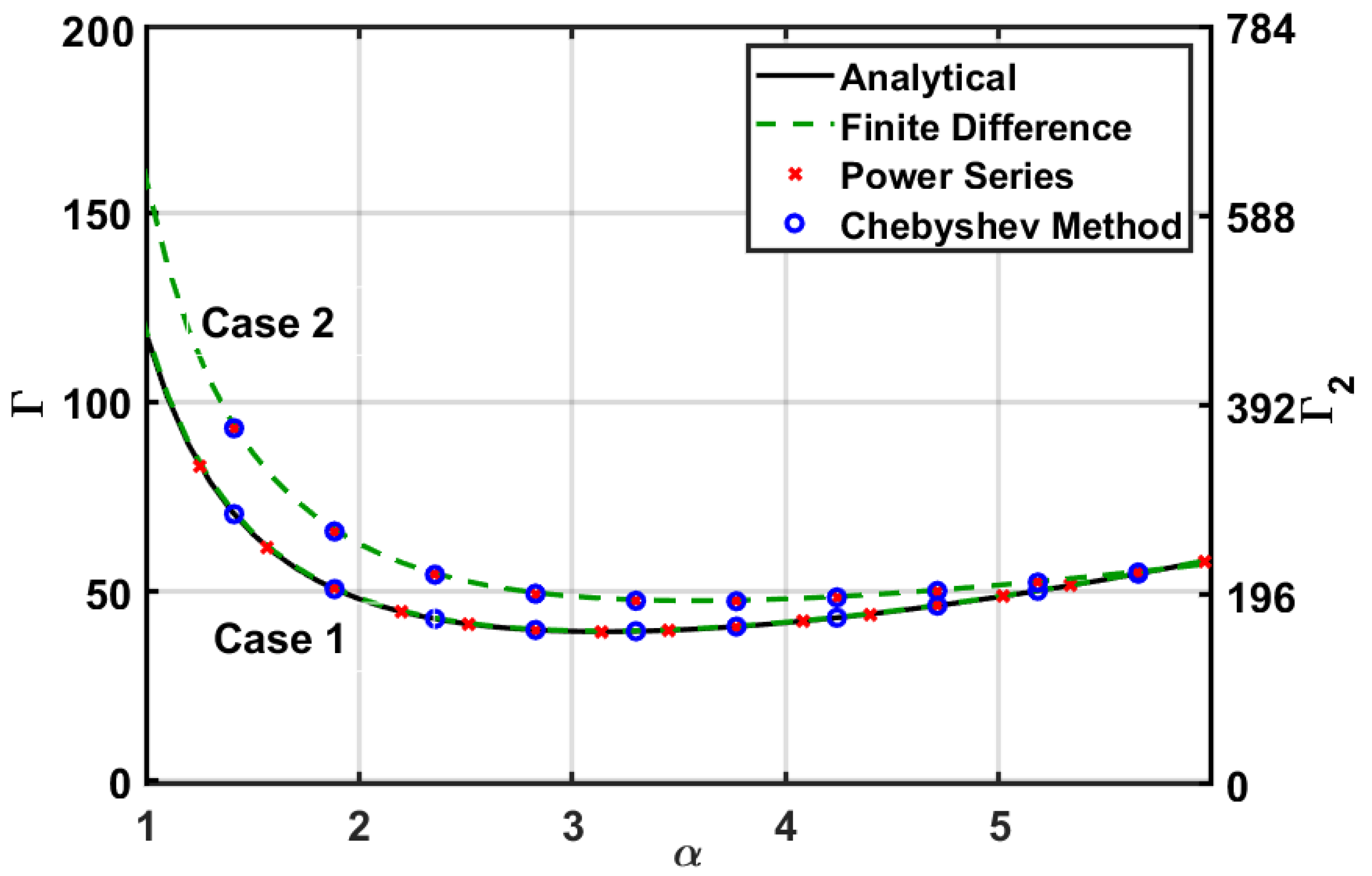
4. Solution Techniques

4.1. Power Series

The system in Equation (10) will be solved in three steps. First, by considering the case of $\lambda =0$ and $g=0$. Second, $\lambda =0$ and $g\ne 0$. Lastly, a non-zero $\lambda$ and g. For the first two cases where $\lambda =0$, the solution can be obtained using a power series expansion. In order to do this, the system is simplified to one equation in terms of $\Theta$.

$$\left\{\begin{array}{cc}\hfill & {[D^2-{\alpha }^2]}^2\Theta =\Gamma {\alpha }^2(1+g)\Theta \hfill \\ \hfill & z=0:\Theta =D^2\Theta =0\hfill \\ \hfill & z=1:\Theta =D^2\Theta =0.\hfill \end{array}\right.$$

(11)

Since g is a polynomial, the power series method is well-suited where $\Theta$ is in the following form:

$$\Theta =\sum _{i=1}^n{a}_n{z}^n.$$

The coefficients can be obtained using the resultant boundary conditions at $z=0$ and plugging the power series into Equation (11), collecting like powers of z, and re-normalize everything by with respect to $a_1$. This process yields the following coefficients:

$$\begin{array}{cc}& a_0=a_2=a_4=0,a_5=\frac{{\alpha }^2}{120}\left(12a_3-{\alpha }^2+\Gamma (1+2c_1+3c_2)\right)\hfill \\ & a_{n+4}=\frac{{\alpha }^2}{(n+4)(n+3)(n+2)(n+1)}[2(n+2)(n+1)a_{n+2}-{\alpha }^2{a}_n+\hfill \\ & \Gamma \left(a_n(1+2c_1+3c_2)-a_{n-1}(2c_1+6c_2)+3c_2{a}_{n-2}\right)].\hfill \end{array}$$

Note that the recursive formula for $a_{n+4}$ is a function of $a_3$. In order to determine $a_3$, the boundary condition $D^2\Theta =0$ at $z=1$ is used to solve for $a_3$. The truncated power series for $D^2\Theta$ will take on the form:

$$D^2\Theta ={\varphi }_1+a_3{\varphi }_2=0\stackrel{}{\to }{a}_3=-\frac{{\varphi }_1}{{\varphi }_2}$$

where $a_3$ can be factored out of ${\varphi }_2$ and explicitly solved. The boundary condition for $\Theta =0$ at $z=1$ is then used to numerically solve for $\Gamma$ as a function of $\alpha$. Due to expanding the power series at $z=0$, high accuracy requires more terms. Truncating the power series to 30 terms results in a maximum percent error of $1.92\times {10}^{-13}$ as compared to the analytical solution for Case 1 for wavenumbers from 1 to 6.

4.2. Chebyshev Method

Next, a spectral expansion in Chebyshev polynomials is used to solve the system of ODEs given in Equation (10). A detailed description of the method is provided in Ref. [26], and thus, a brief overview is provide here. Employing the Chebyshev technique requires shifting the domain to the Chebyshev domain (−1, 1) and expressing the variables as a finite expansion of Chebyshev polynomials:

$$W=\sum _{k=0}^{N+2}{W}_k{T}_k\left(z\right)\mathrm{and}\Theta =\sum _{k=0}^{N+2}{\Theta }_k{T}_k\left(z\right).$$

A weighted inner product with $T_k$ is applied to each equation and converted to a generalized eigenvalue problem.

$$\left(\begin{array}{cc}{D}_2-{\alpha }^{2}I& {\alpha }^2(1+g)I\\ B{C}_1& 0...0\\ B{C}_2& 0...0\\ 0& D_2-{\alpha }^{2}I\\ 0...0& B{C}_3\\ 0...0& B{C}_4\end{array}\right)\left(\begin{array}{c}W\\ \Theta \end{array}\right)=\Gamma \left(\begin{array}{cc}0& 0\\ 0...0& 0...0\\ 0...0& 0...0\\ \frac{d{T}_b}{dz}& -\lambda D\\ 0...0& 0...0\\ 0...0& 0...0\end{array}\right)\left(\begin{array}{c}W\\ \Theta \end{array}\right)$$

where $D_2$ are I are the Chebyshev matrix representation of $D^2$ and identity matrix, respectively. The final eigenvalue system can be solve by passing the matrices through a standard eigenvalue solver, e.g., Matlab’s “eig” subroutine.

Determining the onset of instability requires the smallest eigenvalue. Thus, the wavenumber is swept and a $\Gamma$ determined for every wavenumber. One complexity is added when $\lambda \ne 0$, that is, $\Gamma$ cannot be separated explicitly as an eigenvalue. In order to overcome this, a ‘test’ $\Gamma$ is supplied to the terms containing $\Gamma$ in the matrix and a ‘new’ $\Gamma$ is solved. This iterative process is done until the ‘test’ $\Gamma$ and the ‘new’ $\Gamma$ converge within a designated value (absolute error <0.001).

4.3. Finite Difference Method

Similarly, finite difference method solves Equation (11) as an eigenvalue problem. Since the case of marginal stability is a steady-state problem, the governing equation is classified as an elliptical differential equation. As such, it must be solved by utilizing an implicit method. A system of differential equations is posed, with the governing eigenvalue equation solved at each grid location. For example, Case 1 yields the following:

$$[D^2-{\alpha }^2{]}^2\left[\begin{array}{c}{W}_1\\ W_2\\ ⋮\\ W_n\end{array}\right]=-{\alpha }^2\Gamma \left[\begin{array}{c}{W}_1\\ W_2\\ ⋮\\ W_n\end{array}\right]$$

(12)

where $[D^2-{\alpha }^2{]}^2$ is the finite difference operator which uses central difference schemes for the various derivatives ($D,D^2,D^3,D^4$) before summing them together $(D^4-4D^3\alpha +6D^2{\alpha }^2-4D{\alpha }^3+{\alpha }^4)$ over the mesh stencil for each equation. The algorithm proceeds as follows: (1) Prescribe the wavenumber, $\alpha$. (2) Fill out operator matrix $[D^2-{\alpha }^2{]}^2$ including boundary conditions listed above. (3) Utilize Matlab’s existing “eig” feature to determine possible eigenvalues for a given operator. (4) Find the lowest positive eigenvalue for $\Gamma$. For Case 3, the presence of $\Gamma$ in the operator requires an iterative guess-and-average procedure similar to that described above for the Chebyshev method.

5. Results

5.1. Case 1: $g=0$ and $\lambda =0$

The first case to consider regarding the system given in Equation (10) is the simplest case of $\lambda =0$ and g = 0. Note as $\lambda$$\stackrel{}{\to }$ 0 the base state temperature gradient, $\frac{d{T}_b}{dz}$$\stackrel{}{\to }$−1, i.e., the conductive limit. For large $\lambda$, the base state approaches that given by Wooding [19]. It is easily demonstrated that the system reduces to Equation (13):

$$\left\{\begin{array}{cc}\hfill & [D^2-{\alpha }^2]W=-{\alpha }^2\Theta \hfill \\ \hfill & [D^2-{\alpha }^2]\Theta =-\Gamma W.\hfill \end{array}\right.$$

(13)

It is worth noting that this system is the system given for the Horton–Rogers–Lapwood problem in [14], albeit a Grashof-type number is used ($\Gamma$) instead of a Rayleigh-type number. The analytical solution is simple: $W=\Theta =sin\left(j\pi z\right)$ and $j=1,2,3,\dots$, if $\Gamma =\frac{{({\left(j\pi \right)}^2+{\alpha }^2)}^2}{{\alpha }^2}$. It is clear that $\Gamma$ has a minimum when $j=1$, leading to critical parameters of ${\Gamma }_c=4{\pi }^2$ and ${\alpha }_c=\pi$. Note that $\Gamma$ includes the effects of $\sigma$, which dictates how the porous medium properties (${\left(\rho c_p\right)}_s$) differ from the fluid properties.

This result can be compared to the three techniques used in in this work and is shown in Figure 4. The signature marginal stability curve is reproduced with all three methods.

Table 2. Relative error of the three different methods compared to the analytical solution.

	Power Series	Chebyshev	Finite Difference
Maximum Error [%]	1.92 $\times {10}^{-13}$	$6.9\times {10}^{-7}$	0.74
RMS Error [%]	$8.6\times {10}^{-14}$	$3.3\times {10}^{-7}$	0.44

shows the relative error for the three methods compared to the analytical solution between wavenumbers 1 and 6. Thirty terms are used for both the power series method and the Chebyshev method. The power series is the most accurate but has the longest run time. The finite difference method can be improved by using finer mesh instead of the relatively coarse mesh of 100 points, however, the 100 grid points gave comparable run times to the Chebyshev method and thus was selected as a baseline.

5.2. Case 2: $g\ne 0$ and $\lambda =0$

$$\left\{\begin{array}{cc}\hfill & [D^2-{\alpha }^2]W=-{\alpha }^2(1+g)\Theta \hfill \\ \hfill & [D^2-{\alpha }^2]\Theta =-{\Gamma }_{2}W\hfill \end{array}\right.$$

(14)

Next, the effects of non-linear density are added and the resulting system is shown in Equation (14). As mentioned previously, when a non-linear base density distribution is used, $\beta$ is different than in Case 1. Thus, a scaling factor is needed to equate the $\Gamma$ from case 1 to the $\Gamma$ in Case 2. The $\Gamma$ for Case 2 will be referred to as ${\Gamma }_2$ and is related to Case one by $\Gamma ={\Gamma }_2\frac{\beta }{{\beta }_2}$.

The above system is solved using the three numerical methods that were validated for Case 1 above. As shown in Figure 4, these methods again are all in agreement in their prediction of the marginal stability curve. Due to the additional terms in Equation (14), the power series method converges slower. The Chebyshev method converges the fastest out of the three methods and thus is used for comparison. To demonstrate the agreement between the finite difference and Chebyshev, the mesh is increase by a factor of 10.

Table 3. Relative error of the power series and finite difference method compared to the Chebyshev method.

	Power Series	Finite Difference
Maximum Error [%]	$0.93$	4.6 $\times {10}^{-3}$
RMS Error [%]	$0.29$	$3.22\times {10}^{-3}$

demonstrates the degree of convergence between the three methods for Case 2.

Figure 4 shows the marginal stability curve shift to a higher $\Gamma$ compared to Case 1, indicating a stabilizing effect. Figure 5 helps provide insight to why the non-linear density profile results in a stabilizing effect. Accounting for non-linear changes in density yields a rapid decrease in the initial density near $z=1$. Thus, there is a lower amount of heavy fluid over-top the lighter fluid at the bottom ($z=0$). The end results is a higher Grashof number occurring at a larger wavenumber. The ${\Gamma }_c$ and ${\alpha }_c$ for Case 2 are 47.51 and 3.57, respectively.

Next, the normalized velocities for each case are compared in Figure 6. The non-linear density base profile causes a shift in the sinusoidal shape toward the top of the domain. The overturning convective velocity currents appears to be biased to where the steepest density gradient occur (see Figure 5). Thus, most of the convective mixing inside the porous media will be shifted towards the top of the domain. In addition, the greater wavenumbers in Case 2 promote tighter convective cell formation. These tighter packed cells will ultimately enhance mixing near the coolant side of the porous media once instability ensues.

5.3. Case 3: $g\ne 0$ and $\lambda \ne 0$

Lastly, Case 3 is investigated given by the system in Equation (10). The solution method for Case 3 provided here is the Chebyshev method due to the robustness and speed of convergence. It is worth noting that two additional complexities are added when $\lambda \ne 0$. (1) The base state temperature becomes an exponential function and (2) the base state temperature gradient, $\frac{d{T}_b}{dz}$, is also an exponential function. As mentioned previously, the iterative approach described in the Solution Techniques section is implemented.

Figure 7 shows the marginal stability curves at various $\lambda$’s. Typical transpirational flow rates result in a $\lambda \approx 0.05$ [6,25]. Thus, $\lambda$ is varied from 0.005 to 0.05. Interestingly, increasing $\lambda$ initially yields a destabilizing effect followed by a stabilizing effect. This is consistent with what was observed Sutton [20] who solved a similar problem to the one in this work (variances include a finite horizontal domain, a linear density Boussinesq approximation, and a different non-dimensionalization). Sutton determined at $\lambda =0.005$ that the onset of instability occurred at 39.42 for a domain with a width twice that of the depth. Here, the minimum point for marginal stability for $\lambda =0.005$ occurs at ${\Gamma }_2=196.49$ which corresponds to a $\Gamma =43.24$. Again, as compared to 39.42, the non-linear density provides a stabilizing effect. Figure 7 also illustrates a shift towards higher wavenumbers, which occurs for increasing $\lambda$. The critical values for the different flow rates are summarized in

Table 4. ${\Gamma }_c$ and ${\alpha }_c$ are shown for the various $\lambda$’s in Case 3.

	${\mathit{\alpha }}_{\mathit{c}}$	${\mathbf{\Gamma }}_{\mathit{c}}$
$\lambda =0.005$	3.81	43.24
$\lambda =0.010$	4.07	40.90
$\lambda =0.025$	4.96	38.89
$\lambda =0.050$	7.31	45.73

. Table 4 clearly shows the effect of increasing the net through-flow, which causes a consistent shift and increase in the wavenumber resulting in tighter convective cells.

Lastly, all cases are compared in Figure 8. The effect of each constituent complexity can be compared to the original HRL solution. First, the non-linear density dependence increases the stability of the system from a critical value of $4{\pi }^2$ to $47.51$. Then the system is destabilized from $47.51$ to $45.73$ by adding a base through-flow of $\lambda =0.05$. The system is however regaining stability by increasing the through-flow velocity as shown in Table 4. An increase in wavenumber is observed from Case 1, 2, to 3.

6. Conclusions

Linear stability analysis was performed for a simplified system modeling transpirational cooling applications. Analysis was performed utilizing three models of increasing detail: Case 1, a Horton–Rogers–Lapwood (HRL) type configuration, Case 2, a HRL configuration with non-linear (cubic) density dependence on temperature, and Case 3, both a cubic density function and a base through-flow velocity. In all cases, linear stability analysis was performed to yield governing equations for the system. These equations were then solved utilizing multiple numerical methods, comparing results from a combination of analytical solutions, finite difference, power series, and Chebyshev methods. Results demonstrated excellent consistency in predictions across these methods.

The addition of a cubic density dependence on temperature had several effects as compared to Case 1 (HRL problem). First, accounting for the non-linear density variation during the transpirational heating process shifts the marginal stability curve to a higher Grashof-type number resulting in increased stability. This is due to sharp density gradients near the top wall decreasing the density such that an overlaying fluid is not heavy as compared to the linear density case. In addition, a shift to higher wavenumbers is observed. The cubic density profile also shifted velocity peak toward the top of the porous media. Finally, Case 3 studied the effects of the addition of a base through-flow velocity—the base flow is in the same direction as the gravity vector. A base through-flow velocity sweep revealed that initially increasing the base through-flow destabilizes followed by a re-stabilizing effect. However, it is worth noting that all base flows for Case 3 considered in this work were more unstable as compared to Case 2, i.e., the highest base velocity resulted in a lower critical Grashof-type number as compared to Case 2. In both Cases 2 and 3, accounting for the non-linear variation in density increases the stability of the system.

The implications of an additional mode of convection (buoyancy-induced convection) is increased mixing, i.e., increased heat transfer inside the porous medium. Accounting for this additional mode of convection in cases where instability ensues is important when it comes to thermal management of the system. Thus, an awareness that sharp density gradients at the top of the domain from non-linear density variation in the system, as well as increased through-flow have a stabilizing effect on the system are pertinent to design and modeling considerations.

References

1. Rannie, W.; Dunn, L.G.; Millikan, C.B. A Simplified Theory of Porous Wall Cooling; Technical Report; Jet Propulsion Laboratory, National Aeronautics and Space: Pasadena, CA, USA, 1947. [Google Scholar]
2. Eckert, E.R.G.; Livingood, J.N. Comparison of Effectiveness of Convection-, Transpiration-, and Film-Cooling Methods with Air as Coolant; National Advisory Committee for Aeronautics, Lewis Flight Propulsion Laboratory: Cleveland, OH, USA, 1954; Volume 1182. [Google Scholar]
3. Eckert, E.R.G.; Drake, R.M., Jr. Analysis of Heat and Mass Transfer; McGraw-Hill: New York, NY, USA, 1972. [Google Scholar]
4. Hermann, T.; McGilvray, M. Analytical solution of flows in porous media for transpiration cooling applications. J. Fluid Mech. 2021, 915, A38. [Google Scholar] [CrossRef]
5. Choi, S.; Scotti, S.; Song, K.; Ries, H.; Choi, S.; Scotti, S.; Song, K.; Ries, H. Transpiring cooling of a scram-jet engine combustion chamber. In Proceedings of the 32nd Thermophysics Conference, Atlanta, GA, USA, 23–25 June 1997; p. 2576. [Google Scholar]
6. Langener, T.; Von Wolfersdorf, J.; Steelant, J. Experimental investigations on transpiration cooling for scramjet applications using different coolants. AIAA J. 2011, 49, 1409–1419. [Google Scholar] [CrossRef]
7. Zhu, Y.; Yan, S.; Zhao, R.; Jiang, P. Experimental investigation of flow coking and coke deposition of supercritical hydrocarbon fuels in porous media. Energy Fuels 2018, 32, 2941–2948. [Google Scholar] [CrossRef]
8. Ifti, H.S.; Hermann, T.; McGilvray, M. Flow characterisation of transpiring porous media for hypersonic vehicles. In Proceedings of the 22nd AIAA International Space Planes and Hypersonics Systems and Technologies Conference, Orlando, FL, USA, 17–19 September 2018; p. 5167. [Google Scholar]
9. Dahmen, W.; Gotzen, T.; Müller, S.; Rom, M. Numerical simulation of transpiration cooling through porous material. Int. J. Numer. Methods Fluids 2014, 76, 331–365. [Google Scholar] [CrossRef] [Green Version]
10. Wang, J.; Han, X. Numerical investigation of transpiration and ablation cooling. Heat Mass Transf. 2007, 43, 275–284. [Google Scholar] [CrossRef]
11. Glass, D.E.; Dilley, A.D.; Kelly, H.N. Numerical analysis of convection/transpiration cooling. J. Spacecr. Rocket. 2001, 38, 15–20. [Google Scholar] [CrossRef] [Green Version]
12. Horton, C.; Rogers, F., Jr. Convection currents in a porous medium. J. Appl. Phys. 1945, 16, 367–370. [Google Scholar] [CrossRef]
13. Lapwood, E. Convection of a fluid in a porous medium. In Mathematical Proceedings of the Cambridge Philosophical Society; Cambridge University Press: Cambridge, UK, 1948; Volume 44, pp. 508–521. [Google Scholar]
14. Nield, D.A.; Bejan, A. Convection in Porous Media; Springer: Cham, Switzerland, 2006; Volume 3. [Google Scholar]
15. Prats, M. The effect of horizontal fluid flow on thermally induced convection currents in porous mediums. J. Geophys. Res. 1966, 71, 4835–4838. [Google Scholar] [CrossRef]
16. Barletta, A.; Celli, M.; Rees, D.A.S. Darcy–Forchheimer flow with viscous dissipation in a horizontal porous layer: Onset of convective instabilities. J. Heat Transf. 2009, 131, 072602. [Google Scholar] [CrossRef]
17. Celli, M.; Impiombato, A.N.; Barletta, A. Buoyancy-driven convection in a horizontal porous layer saturated by a power-law fluid: The effect of an open boundary. Int. J. Therm. Sci. 2020, 152, 106302. [Google Scholar] [CrossRef]
18. Barletta, A.; Celli, M. The Horton–Rogers–Lapwood problem for an inclined porous layer with permeable boundaries. Proc. R. Soc. A Math. Phys. Eng. Sci. 2018, 474, 20180021. [Google Scholar] [CrossRef] [PubMed] [Green Version]
19. Wooding, R. Rayleigh instability of a thermal boundary layer in flow through a porous medium. J. Fluid Mech. 1960, 9, 183–192. [Google Scholar] [CrossRef]
20. Sutton, F.M. Onset of convection in a porous channel with net through flow. Phys. Fluids 1970, 13, 1931–1934. [Google Scholar] [CrossRef]
21. Homsy, G.M.; Sherwood, A.E. Convective instabilities in porous media with through flow. AIChE J. 1976, 22, 168–174. [Google Scholar] [CrossRef]
22. Partha, M. Nonlinear convection in a non-Darcy porous medium. Appl. Math. Mech. 2010, 31, 565–574. [Google Scholar] [CrossRef]
23. RamReddy, C.; Naveen, P.; Srinivasacharya, D. Influence of non-linear Boussinesq approximation on natural convective flow of a power-law fluid along an inclined plate under convective thermal boundary condition. Nonlinear Eng. 2019, 8, 94–106. [Google Scholar] [CrossRef]
24. Lemmon, E.; Bell, I.H.; Huber, M.; McLinden, M. NIST Standard Reference Database 23: Reference Fluid Thermodynamic and Transport Properties-REFPROP, Version 10.0; Standard Reference Data Program; National Institute of Standards and Technology: Gaithersburg, MD, USA, 2018. [Google Scholar]
25. May, L.; Burkhardt, W.M. Transpiration Cooled Throat for Hydrocarbon Rocket Engines; Technical Report; Aerojet Propulsion Div: Sacramento, CA, USA, 1991. [Google Scholar]
26. Harfash, A. Numerical methods for solving some hydrodynamic stability problems. Int. J. Appl. Comput. Math. 2015, 1, 293–326. [Google Scholar] [CrossRef] [Green Version]
Figure 1. Simplified model of the transpirational cooling process.
Applsci 11 11766 g001
Figure 2. Reduced density ( ρ ρ c ) versus reduced temperature ( T * T c ) for hydrogen (blue circle) and methane (red square) for a sweep of reduced pressures range from 1 to 5. The black solid line is a third order approximation of the thermodynamic data.
Applsci 11 11766 g002
Figure 3. Dimensionless density versus dimensionless temperature is shown (red-dashed line) for methane at typical conditions of T 0 = 105 K and T w = 755 K [25]. A third order polynomial is used to fit the data (black solid line). The linear fit is shown as the blue small-dashed line.
Applsci 11 11766 g003
Figure 4. The stability curves are illustrated for Case 1 and 2 for the three different solution techniques. The right axis plots Γ 2 where Γ 2 = β 2 β Γ .
Applsci 11 11766 g004
Figure 5. Density versus domain depth is plotted for the non-linear density (red-dashed line) and linear density (blue small-dashed line) profiles.
Applsci 11 11766 g005
Figure 6. The normalized velocity profiles are shown for Case 1 and 2 for the state of marginal stability.
Applsci 11 11766 g006
Figure 7. Marginal stability curves for Case 3 are shown for different base flows, λ .
Applsci 11 11766 g007
Figure 8. The marginal stability curve are plotted for Case 1, 2, and 3 when λ = 0.05 .
Applsci 11 11766 g008