Cyber-Physical LPG Debutanizer Distillation Columns: Machine-Learning-Based Soft Sensors for Product Quality Monitoring

Featured Application

The outcomes of this work can be applied to forecast C5 content in debutanizer columns based on data obtained by a few pressure and temperature sensors. In addition, the proposed visualization can be used as a model global explanation, highlighting opportunities regarding feature selection, the most important features guiding the forecasts, and threshold values within which the forecasting model can operate.

Abstract

Refineries execute a series of interlinked processes, where the product of one unit serves as the input to another process. Potential failures within these processes affect the quality of the end products, operational efficiency, and revenue of the entire refinery. In this context, implementation of a real-time cognitive module, referring to predictive machine learning models, enables the provision of equipment state monitoring services and the generation of decision-making for equipment operations. In this paper, we propose two machine learning models: (1) to forecast the amount of pentane (C5) content in the final product mixture; (2) to identify if C5 content exceeds the specification thresholds for the final product quality. We validate our approach using a use case from a real-world refinery. In addition, we develop a visualization to assess which features are considered most important during feature selection, and later by the machine learning models. Finally, we provide insights on the sensor values in the dataset, which help to identify the operational conditions for using such machine learning models.

1. Introduction

Petroleum refineries receive crude oil of different provenances with their specific characteristics. The inlet crude oil feedstock is transformed into final products through multiple processes. Each process provides products whose qualities are prescribed by different standards, such as the Liquefied Petroleum Gas (LPG), a mixture of hydrocarbon gases used in heating appliances and vehicles. The final mixture product usually contains 48% propane, 50% butane, and up to 2% pentane (hereafter, also referred to as C5) which is developed based on local regulations and composition requirements, the intended use, and even seasonal limitations (e.g., a higher proportion of propane is used in winter due to its evaporation point).

To achieve the desired quality, the LPG obtained from crude oil distillation must undergo several processes to remove impurities. One of these purification processes is debutanization, which removes C5. To ensure the final mixture meets the specification standards, samples are taken in various stages of the refinement and purification process and undergo lab analysis. Results are passed on to production engineers so that they can adjust process settings if required. However, lab analysis may take up to several hours to be completed and is not conducted every day, causing the identification of an already existing off-specs situation to be delayed. This, in turn, makes recovery harder, since the sooner an off-spec situation is identified and resolved, the better it is for the recovery efforts in terms of both time and cost. Hence, there is a need for early (or ideally real-time) identification of situations where C5 content exceeds specifications. This brings a strong motivation to create a model-based approach for a cognition module supporting the operation which alerts of an C5 off-spec situation, and enables real-time decision-makings based on such alerts.

Currently, several approaches to estimate debutanization process outcomes exist. Among them, Aspen HYSYS (https://www.aspentech.com/en/products/engineering/aspen-hysys (accessed on 23 October 2021)) uses mathematical models to simulate a debutanizer unit and predict process outputs. Such simulation models frequently use elaborate math and complicated equations to achieve enough generalization to be applied across different units. Data-driven models overcome limitations regarding equation solving complexity by using past data to learn and produce possible solutions. Although the ability to reuse them across units strongly depends on the model design, once trained, such models can provide forecasts with almost no latency. If forecasts are good enough, the models can acquire frequently insights regarding C5 content in the LPG, for providing ground for earlier off-spec product identification and timely decision-making.

Real-time prediction of C5 content during the debutanization processes provide new insights that guide decision-makings for process monitoring and control. To create machine learning models capable of such forecasts, we use historical sensor data regarding operational temperature and pressure, as well as laboratory results obtained from the samples analysis. Such data and analysis results enable the support of machine-learning model training and evaluation by identifying correlations between sensed conditions and measured outcomes for two purposes: (i) with real-time sensor data, such models can provide real-time C5 content estimates; (ii) with new real-time sensor data and lab analysis data update, the machine-learning model performance is expected to be promoted in time, if retrained with the new data available.

In this paper, we develop machine learning models for a real-world use case, based on sensor data provided by a Tüpras (https://www.tupras.com.tr (accessed on 23 October 2021)) refinery. By examining the actual process in the use case, we found that different debutanizer columns have different features because of their different designs. Moreover, only a few sensors are in the debutanizer column. Most sensor data corresponded to the pipping system that connected the debutanizer column with the condensation unit and the units that follow. We used several debutanizer unit diagrams to understand where the sensors are located, and which sensors are close to the distillation column exit. Temperature and pressure conditions are identified by the ones near the column exit, and hence the first ones placed in the pipes close to the related exit but before the condensation unit. We assume such data provides good insight on how operating conditions relate to extracted samples and measured composition. Furthermore, we observed that there are some cases where both temperature and pressure sensors exist for any given point in the debutanizer column, but at least one of them exists. Considering these limitations, machine learning models are developed to predict C5 content based on the inputs of two sensors (one pressure sensor and one temperature sensor). Finally, we develop two machine learning models that provide predictions based on the data from these two sensors for independent estimate: (i) one that predicts the expected amount of C5 in the LPG; and (ii) one that forecasts whether C5 content is off spec (higher than 2%).

The contribution of this paper is the use of operational temperature and pressure sensor data to develop:

• a machine-learning model to predict C5 content in LPG stream;
• a machine-learning model to predict if C5 content exceeds specification levels

Machine-learning models built using data from a few sensors can be more easily applied to a broad range of debutanizer columns since they impose fewer restrictions on the number of input data sources required to provide forecasts. Thus, we consider that a major strength of our approach is the fact that it relies only on data of two sensors, one measuring pressure and the second one measuring temperature in the debutanizer column-both placed at separate locations within the column.

Along with the development of the aforementioned models, we also provide a prototype dashboard, which provides global explanations to understand which features were considered most relevant during the feature selection, and which features were considered relevant by the forecasting model. In addition, we provide insights on the sensor value distribution in the training set, to understand the model operational limitations.

To evaluate our models, we have used three metrics: two for measuring regression features and one for measuring the classification features. We assess the regression model performance with the Root Mean Square Error (RMSE) and the Mean Absolute Error (MAE). The MAE is not sensitive to outliers and can thus provide a reasonable estimate of the model performance for normal C5 levels. The RMSE penalizes large errors and thus better indicates if out-of-spec measurements were predicted adequately. The classification model performance is measured with the Area Under the Receiver Operating Characteristic Curve (AUC ROC [1]). AUC ROC is invariant to a priori class probabilities, referring to a relevant property when measuring model discrimination power in an imbalanced dataset. After evaluating the models, results show that our approach is applied to effectively provide real-time C5 content predictions in the LPG debutanization process of our given use case.

The rest of this paper is structured as follows: Section 2 presents related work. Section 3 describes a Tüpras refinery use case, and Section 4 introduces the features created for the C5 content forecasting model, as well as the way to develop and evaluate these models. Section 5 presents the experiments we performed and the obtained results. Finally, Section 6 offers our conclusions and provides an outline for future work.

2. Related work

2.1. Distillation Process-Related Models

Debutanizer columns are an important part of several processing units in oil refineries. Therefore, the objective of the online composition of debutanizer outlet streams is to maximize the production of LPG while meeting the corresponding quality standards. Currently, the quality of the debutanizer output is measured via laboratory analysis. Hence, changes in the quality are identified only upon the analysis of the sample, which may take several hours. Therefore, to maintain the quality of the product within the predefined specifications, it is of imperative importance to predict the top and bottom outputs of the debutanization process precisely [2].

To realize this objective, Ref. [3] identifies three major approaches to develop the required models: (i) first-principle (a.k.a. fundamental) models, which consider mass, energy, and momentum principles and equations to provide a forecast; (ii) machine learning models, which are created by training an algorithm on input-output data of the process; and (iii) hybrid models, which combine both the fundamental and the empirical models.

First-principle models involve sets of non-linear differential equations (usually in the order of ${10}^2$ or ${10}^3$ non-linear differential equations) and a comparable number of algebraic equations [4,5]. The equations usually take into account the global balance of matter, partial balances of matter, pressure, temperature, flow, reflux policies, and the relationship between component concentrations at different levels of the distillation column [3,6]. Although additional information regarding the structure of the distillation column can further enhance such models (e.g., the number of trays in a column or the column hydraulics [7]) with the increasing computational complexity of such models.

To alleviate the computational needs, simplified distillation column models have been proposed [8,9], at the expense of an increased error whose applicability often restricted to a single column [10]. These models are usually implemented in Advanced Process Control systems (APC), such as a Multivariable Model Predictive Control (MPC), for managing relevant process variables and their dynamics. The equations mentioned above govern the control logic between variables. Algorithms that perform matrix computations are used to solve such system dynamic models with multiple variables simultaneously. In addition to their computational complexity, the usefulness of such models is constrained to the model assumptions, e.g., sensor colocation points [11].

Data-driven models provide an alternative modeling approach for developing the forecast models [12]. In particular, machine learning models are developed based on the prior knowledge of the physical processes for creating good features of model outputs. The models are trained with the collected data from the actual operations of the unit: (1) The raw data are transformed into a dataset for developing models which perform features that reflect different dynamic features for the raw data variables; (2) Through the developed models, observed outputs are generated through the feature vectors. Through such model features, the machine learning models can accurately learn non-linear features from the data, even when some noises exist in the data [13].

Hybrid models arise from the combination of the first-principle and data-driven models [14]. Such models are used to retain the theoretical knowledge of the process, which is mirrored in equations. In contrast, the data-driven models can augment such knowledge using data, and can be used to model parts of the process that are hard to formulate and would otherwise require overly complex first-principle models [3,15]. Hybrid models have been implemented widely in various chemical processes such as batch distillation [16], reactive distillation [17], and polymerization process [18,19]. However, only a handful of models have been implemented in continuous distillation columns.

In the literature, there are some attempts to model continuous distillation processes in refineries. Such attempts not only include debutanizer columns [11,20], but also various other units such as Crude Distillation Units (CDU) [21,22] and Fluid Catalytic Crackers (FCC) [23,24]. Among the models developed for debutanizer columns, we find the artificial neural networks (ANN) [22,25,26], partial least square regression [27,28], support vector regression (SVR) [22,27], principal component regression [29], supervised latent factor analysis [30,31], probabilistic regression [32], and state-dependent autoregressive model with exogenous variables [33].

To evaluate C5 and C4 product concentrations in the debutanizer column, Ref. [3] created a dynamic neural model that acts as a soft sensor based on the data provided. In a similar manner, Ref. [34] developed an ANN model to predict LPG composition at the top and bottom of a distillation column, comparing its performance to a partial least squares model. A comparison between different models was also performed by [26], which developed multiple linear regression, principal components regression, and neural networks models for a debutanizer column. They concluded that the performance of such models was superior to least square regression models and support vector regression models reported in the literature. Finally, Ref. [35] aimed to identify the governing equations regarding a distillation column using a white-box machine-learning approach.

Cyber-physical systems describe systems that integrate the physical processes into the digital world, where monitoring and analytics can be performed [36,37]. A standard abstraction model considers three significant layers: physical, cybernetic, and an interface between both [38]. The concept of cyber-physical systems has been successfully implemented in petrochemical plants [39].

This paper highlights the importance of artificial intelligence applications compared to traditional analytic methods based on mathematical models. It proposes a cyber-physical integration using machine-learning models to provide real-time LPG C5 content estimates based on streamed sensor data. In our use case, sensor data regarding pressure and temperature was available only from a few sensors at the top of the debutanizer column; hence, such models could not be replicated. Nevertheless, we have acknowledged the algorithms described in the related work and implemented models based on them and our set of features.

2.2. Explainable Artificial Intelligence

The machine learning models are growing in complexity and sophistication providing accurate forecasts based on historic data. At the same time, there is an increasing need to understand the logic behind such models, to comply with regulatory requirements, and provide ground for responsible decision-making [40,41]. Insights on the process followed by such models when applying operations on the input to provide a forecast enable a decision about whether such forecasts can be trusted or not [42,43]. To respond to such challenges, research on techniques, approaches and visualizations is done in a sub-field of artificial intelligence, known as Explainable Artificial Intelligence (XAI).

Multiple taxonomies were proposed to categorize the different XAI approaches. Arrieta et al. distinguish between transparent models and post-hoc explainability techniques, dividing the last category into model-agnostic and model-specific approaches [44]. Transparent models are also known as inherently interpretable or white-box models, while the models that do not fall into this category, are considered opaque or black-box models [45]. A more elaborate taxonomy was proposed by Das et al. [46], who considered dividing XAI techniques based on three criteria: scope (considering global or local explanations), methodology (if the technique focuses on the input data or model parameters), and usage (if is model-agnostic or model-specific). Regarding the scope, local explanations provide insights regarding a particular forecast, while global explanations attempt to describe the overall model behavior [47].

When providing global explanations for models trained on tabular data, a frequent model-specific approach is to consider the feature weight in the model to determine the feature relevance ranking. Model-agnostic alternatives have been devised by several authors using surrogate models [48,49,50]. Although much research has been done on explaining model behavior, less research was invested towards crafting comprehensive explanations with insights regarding the data and the model creation process. Part of this void was addressed by MELODY (MachinE-Learning MODel SummarY) [51], and SUBPLEX [52], which connect local explanations to data analytics either summarizing insights regarding the whole dataset or a relevant subpopulation. INFUSE [53], on the other side, focused on providing explanations regarding the feature selection process, and the influence of different feature selection strategies on it. Although INFUSE takes into account a process of cross-validation, it does not bind it to the resulting model and any model related explanations.

Visual interpretations are considered particularly effective to explain the model forecasting rationale [54]. Although much work was invested towards developing XAI techniques, some researchers consider not enough research was invested on making such explanations end-user-centered [55,56]. Visual explanations comprehend insights regarding the dataset and feature contributions at a local and global level. Scatterplots are frequently used to visualize data distribution, using some dimensionality reduction technique to map the high-dimensional dataset into two dimensions [57,58]. Color-coded instances are frequently used in classification tasks, and interactive interfaces provided, to enable the user focus on specific instances and conduct further research [47]. To represent feature contributions, horizontal bar plots [52,59,60], breakdown plots [61,62], heatmaps [63,64], Partial Dependence Plots [65], or Accumulated Local Effects Plots [66] are used.

In this research, we complemented our model development with a dashboard that provides insights into the most informative features within the dataset, when considering feature selection, while also informing their relevance from the model point of view. In addition, we inform the value ranges of each sensor’s readings found in the dataset. Such values must be taken into account, since the model is able to issue good predictions within the observed ranges, and not outside them.

3. Problem Statement

3.1. Tüpras Refinery

The use case corresponds to a Tüpras refinery located in Izmit, which began oil production in 1961 and currently has a design capacity to process 11.3 million tons of crude oil per year. The crude oil is supplied from four countries: Iran, Iraq, Russia, and Saudi Arabia. Each of these crude oil feedstocks have different characteristics such as density, sulfur content, and impurities. The refinery complies with Euro 5 standards [67] and produces mostly diesel, gasoline, and LPG. The entire refining unit consists of atmospheric and vacuum distillation units, hydrocrackers, fluid catalytic crackers, continuous catalyst regeneration reformers, diesel and kerosene desulphurization units, merox, asphalt units, and sulfur recovery units. In Figure 1, we provide a diagram showing the relation between processing units of this refinery, highlighting the LPG and gas flows. In this research, we focus on the LPG debutanizer units, which is implemented for the atmospheric distillation process. Although feedstock changes regularly, experts pointed out that they do not display much difference in light hydrocarbons content regardless of the crude oil provenance. The atmospheric distillation process ameliorates this difference before the LPG enters the debutanizer unit. Given that the concentration of pentanes does not depend on the crude oil provenance, we consider it as a specific function of the debutanization process which is a distillation process with two control variables: pressure and temperature.

3.2. Debutanization Process

The debutanization process is a fractional distillation process that aims to recover the light gases ($C1-C4$) and the Liquefied Petroleum Gas ($LPG$) from the overhead distillate coming from the distillation unit [26]. This distillation process aims to separate liquid components by heating a liquid to vapor, condensing the vapor back to liquid to purify or separate it. To that end, three components are required: (1) a distillation column (used to separate a liquid mixture into its fractions based on the differences in volatilities); (2) a reboiler (used to provide the necessary vaporization of the distillation process); (3) a condenser (used to cool and condense the overhead vapor).

The $CH4$ (methane) component exists in the feedstock with the other alkane compounds, with the $C4H10$ (butane) fraction only gaining its freedom when the vaporized gas condenses inside the array of valve trays that line the interior of the debutanizer column. Based on thermal unit conversion technology, the butane is efficiently siphoned from the raw feed. To achieve this, the boiling point of butane is used as a reference point to determine temperature and pressure conditions. Pure butane condenses in the debutanizer column when the architecture of the column locks in the mandated variables, so few impurities can form. Similarly, propane, ethane, and methane are liberated and refined as valuable fuel sources in the other alkane processing columns.

Pressure is frequently considered the most relevant distillation control variable since it affects column temperatures, product relative volatilities, condensation (and therefore the distillate composition), and cooling and energy requirements [68]. Pressure controls are usually integrated into the condensation system, and therefore both need to be considered simultaneously. The satisfactory operation of the distillation column requires steady pressure, and pressure changes must be introduced slowly and steadily. In a mass balance control, higher distillation column pressures reduce the relative volatility between the components, increasing the molar flow rates, the condensation rate, and therefore the amount of reflux [69]. Conversely, low pressures can prevent condensation and thus prevent a successful distillation. In atmospheric distillation columns, the condensation rate can be controlled through the temperature too [70].

The control of condensate temperature enables additional control over vapor and liquid product split. Changes in the temperature usually correlate with changes in the product composition [71]. In particular, differential temperature control considers that given temperature measurements at two different points of the distillation column, the temperature difference between both remains constant regardless of the pressure changes. Variations in the temperature difference thus signal changes in the composition profile of the product [72]. It must be noted that vapor enters the distillation condensers at a saturation temperature.

Given the importance of the pressure and temperature variables in the distillation process, it is critical to determine the best placement of the sensors to enable adequate and timely insights into the process. The distillation column pressure is usually measured in vapor spaces at the reflux accumulator and the top of the column. The column temperature is usually measured nearby the condenser to avoid a dynamic lag associated with the reflux drum. The temperature sensor placement follows two criteria: the linearity of the response (where the steady-state responses to a positive and negative change in the corrective action are most similar), and the maximum sensitivity to product composition. In addition, experts consider that the best temperature control points are where the most extensive and symmetrical temperature variations are observed [70].

Please note that it is widely considered that reflux needs to be controlled to achieve on-spec production, Ref. [70] points out that such reasoning originates from a distillation column design practice, where reflux is increased until the product achieves a particular specification given several stages for which the distillation column is designed. However, the same author clarifies that the primary consideration for introducing reflux into a tray tower is to achieve good hydraulics and thus avoid premature flooding and entrainment. Although the absence of a reflux drum makes the condensation rate a slave of the top product rate, the reflux control provides additional means to increase the purity of the overhead product keeping out the heavier fraction from the stream of vapor that leaves the top of the tower.

Modeling a distillation column is a complex process as it involves various non-linearities and includes multiple variables with interactions between them [73]. In the Tüpras refinery, there is an abundance of sensors to monitor the entire debutanization processes. Data from these sensors include measurements of input and output flows, temperatures, and pressures across the whole refinery. These are used in feedback loops to maintain the process stable and control the system dynamics close to the set-point values that the process engineers have selected for seamless plant operation. Although rich sensor data exists, we only obtained the data from the temperature and the pressure sensors on the top of the debutanizer columns. Although a limited number of sensors was provided, our proposed approach presents excellent results as shown in Section 5.

3.3. Relevant Physical and Chemical Principles and Laws

In our use case, we have sensor data for the temperature and pressure measurement. To formalize meaningful features enabling the models to predict C5 content, we have considered the following laws and equations from physics:

• Raoult’s law states that the total pressure of a component equals the vapor pressure of its pure components multiplied by their mole fraction (see Equation (1));
• Antoine’s equations provide a relationship between the vapor pressure of a pure component and three empirically measured constants at a given temperature (see Equation (2));
• Combined Gas Law states that the ratio of the product of pressure and volume and the absolute temperature of a gas equal a constant (see Equation (3));
• Clausius-Clapeyron relation describes pressure at a given temperature T₂ if the enthalpy of vaporization and vapor pressure are known at some other temperature T₁ (see Equation (4))

$$P=P_1·x_1+\dots +P_n·x_n$$

(1)

Equation (1): Raoult’s law. P refers to pressure, x refers to mole fraction, and the n indicates different mixture components.

$$lo{g}_{10}P=\frac{A˘B}{C+T}$$

(2)

Equation (2): Antoine’s equation. P refers to pressure, T refers to temperature. A, B, C are empirical, component specific constants.

$$k=\frac{P·V}{T}$$

(3)

Equation (3): Combined Gas Law equation. P refers to pressure, V refers to volume, and T refers to temperature. k is a constant.

$$ln\left(\frac{P_1}{P_2}\right)=-\frac{L}{R}·\left(\frac{1}{T_2}-\frac{1}{T_1}\right)$$

(4)

Equation (4): Clausius-Clapeyron relation. P refers to pressure, T refers to temperature, L is the specific latent heat of the substance, and R is the specific gas constant.

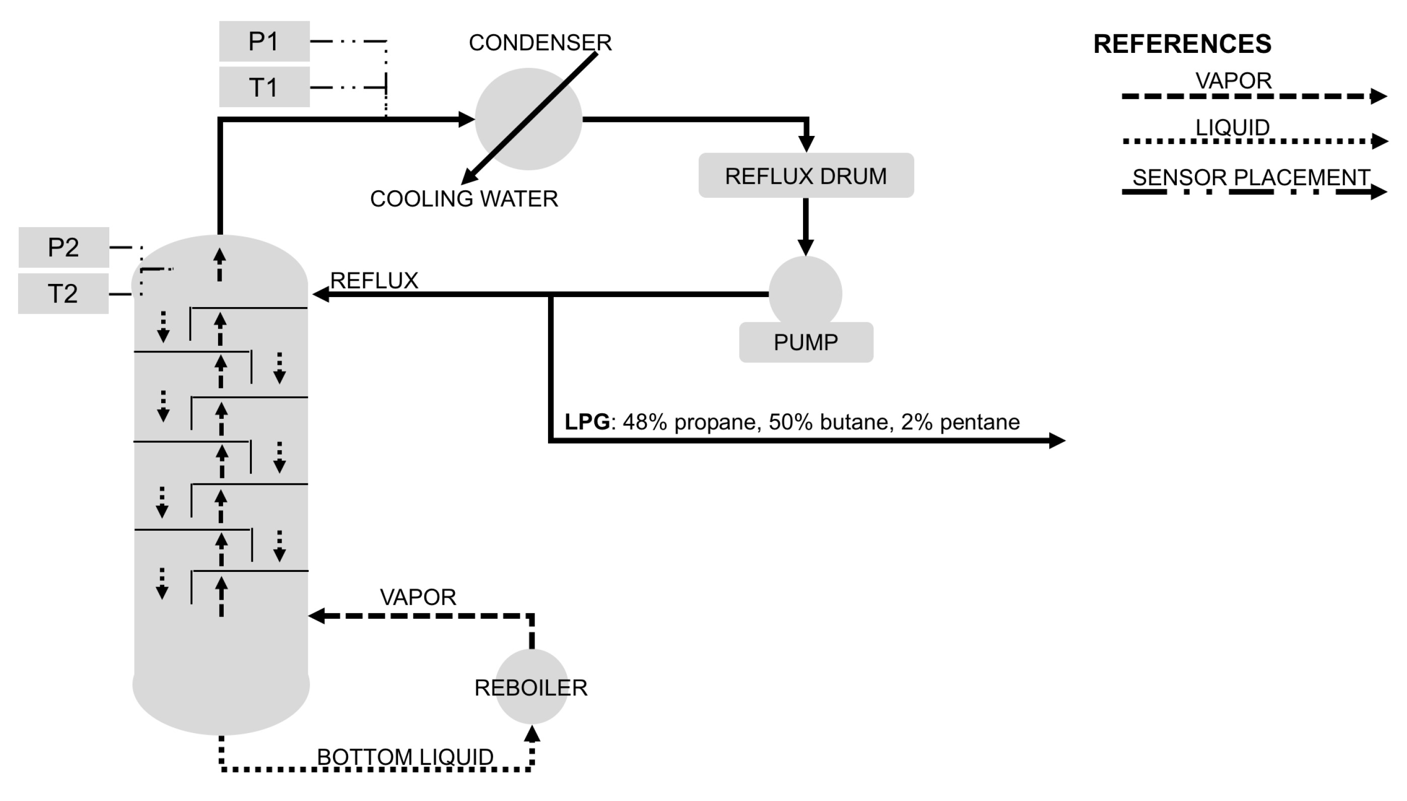
For the case study, we obtained data from sensors P1 and T2 of the debutanizer unit (in the Figure 1); while we missed sensor readings from T1 and P2.

Not having both temperature and pressure at a given point of the debutanizer column prevents us from using the Ideal Gas Law equation to compute the gas molar weight (see Equation (5)) of the mixture. The gas molar weight could provide further insights on the mixture composition using the gas molar weight equation (see Equation (6)). The gas molar weight equation expresses that the gas molar weight equals to the sum of the molar weights of the pure components multiplied by their mole fraction.

$$P·V=n·R·T$$

(5)

Equation (5): Ideal Gas Law. P stands for pressure, V stands for volume, n represents the amount of substance, R is the ideal gas constant, and T corresponds to the temperature.

$$M=M_1·x_1+\dots +M_n·x_n$$

(6)

Equation (6): Molar weight equation. M stands for molar weight, x represents mole fractions, while the subindexes indicate different mixture components.

LPG specifications require LPG to have a mixture of propane and butane, with no more than 2% of the volume of five carbon components (C5) and no more than 5% of the volume of two and five carbon components (C2 and C5). Though many possible components have two and five carbons, we decided to approximate them as a single pure component. Considering the laws, equations, and restrictions described above, we can derive a set of equations, which provide meaningful cues on the expected mixture composition, and thus drive better forecasts. e.g., from Equation (1) and approximating the LPG composition to the four elements described above, we obtain that C5 proportion can be expressed as Equation (7). Although pressure is known from the sensor readings (P1), we do not know the exact proportion of propane and butane. We also miss sensor data regarding the temperature at the same point where the pressure is sensed (T1). Considering that the relationship between temperature and pressure is linear, and given a snapshot of sensor data, we approximate T1 based on P1 and T2. Such an approximation allows us to compute saturation pressures for pure LPG components based on Antoine’s equations (see Equation (2)). Considering various scenarios of possible LPG composition, we compute features (see Section 4.3) signaling expected pressure for given conditions and how it compares to the pressure sensed in the debutanizer unit. When considering the constants for Antoine’s equations, we approximated two carbon hydrocarbon elements with methyl-disulfide (C₂H₆S₂), and five carbon hydrocarbon elements with pentane (C₅H₁₂)). When doing so, we considered the vaporization temperature and sulfur content (sulfur is removed in later stages).

$$x_{C5}=\frac{P-(P_B·x_B+P_P·x_P+P_{C2}·(1-x_B-x_P))}{P_{C5}-P_{C2}}$$

(7)

Equation (7): Estimated C5 content. We obtain P from sensor data, P_i can be computed based on a given temperature, x_B and x_P can be approximated to LPG specification, or other useful values.

4. Methodology

4.1. Data Preparation

To realize the proposed machine learning models, we used data provided by Tüpras. The data included temperature and pressure sensor data, and 263 laboratory measurements (167 measurements from the debutanizer Unit A, and 96 from the debutanizer Unit B), all sampled simultaneously at irregular day intervals. We consider that the irregular sampled data should not affect the machine-learning model training since temperature and pressure sensor inputs are used to estimate LPG C5 content. As described in Section 3, experts informed us that light components, such as C5, do not vary much between feedstocks. The debutanizer follows a previous distillation phase, where LPG is separated from the rest of crude oil derivatives. Therefore, the debutanizer’s operational pressure and temperature are used to influence the observed LPG C5 concentration.

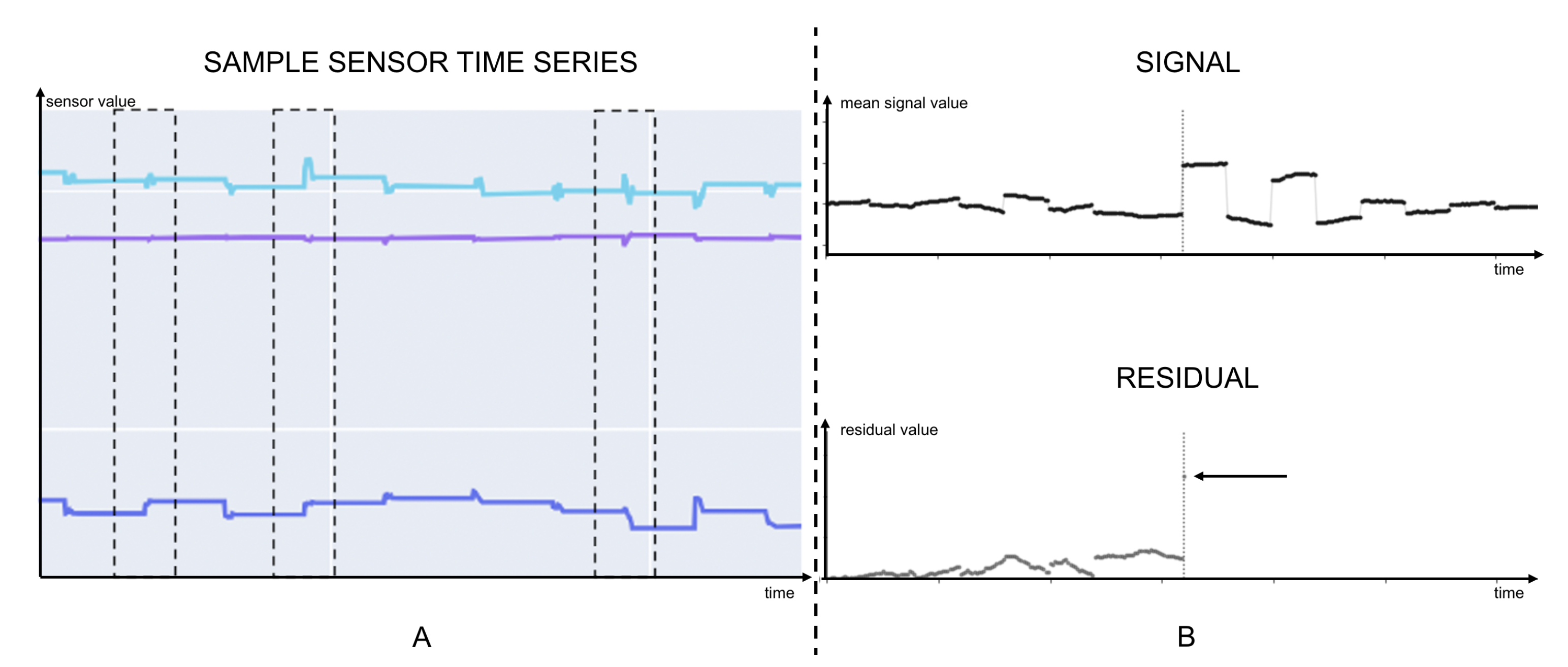
We found that sensor data were available at different frequencies when creating the dataset for training machine-learning models. Although some sensors provided readings every five seconds, others provided data at a minute level. We thus resampled all sensor data at a minute level and set all values to second zero. When resampling, we considered the last sensor reading. We chose to impute values using forward filling for missing values, considering that missing sensor readings are most likely to have a value similar to the last one observed. Since we had no information regarding set-point configurations on past operations, we ran a change level detection algorithm on sensor reading time series. The algorithm computed the mean of the past sensor readings and compared the value to the new sensor reading. If the new reading was above a certain threshold, we considered a new set-point was set. We empirically tried different threshold values and obtained the best results, corroborated with plots manual inspection, by setting it to 4%. In Figure 2A, we provide an example of three time series of sensor data, enclosing some level changes within dashed squares. In Figure 2B, we show two plots that illustrate how the change level detector works. The plot at the top shows average signal values, while the plot at the bottom shows the residual, computed as the difference between the new sensor reading and the average signal value.

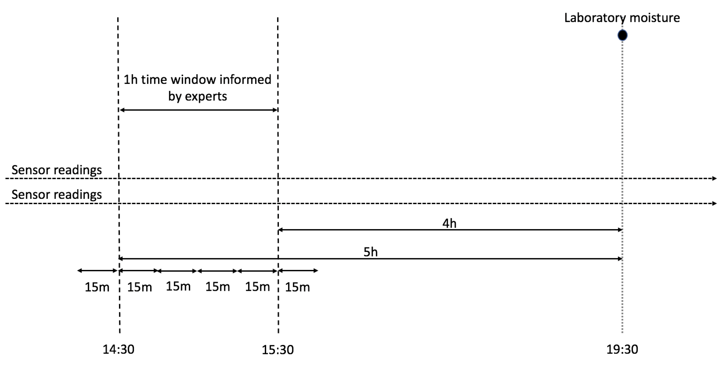
Experts instructed us that the timestamps from laboratory samples did not match sensor data timestamps. To match them, timestamps from laboratory samples had to be transposed four to five hours earlier. Since accurate data regarding time transposition was missing, we decided to consider sensor values measured in 15 minutes slots for a time range of an hour and a half (see Figure 3). Since operational conditions change when a new set-point is given, we computed the median sensor value since the last change level detected and the upper bound time considered to match the laboratory reading.

4.2. Data Analysis

To perform our research, we focused on the data provided from the two LPG debutanizer units. We obtained a total of 263 laboratory analysis results: 167 for Unit A and 96 for Unit B. Sensor reading values were attached to them through the procedure described in the previous subsection. We observed that only Unit A had pentane concentrations that exceeded the allowed out-of-specification threshold, reaching a total of 14 off-specification events. We provide the summarized statistics of the sensor readings and target values in

Table 1. Description statistics for sensor and laboratory analysis data obtained for debutanizer Unit A and Unit B.

	Unit A							Unit B
	Mean	Stdev	min	25%	50%	75%	Max	Mean	Stdev	min	25%	50%	75%	Max
P1 (kg/cm2)	7.42	0.29	6.54	7.28	7.43	7.60	8.32	4.98	3.84	0.00	0.00	7.61	8.02	8.78
T2 (°C)	62.66	19.82	0.00	66.17	67.41	69.13	89.70	35.99	30.84	0.00	0.00	58.20	61.38	80.36
C5 (%)	0.63	1.15	0.00	0.02	0.17	0.70	6.52	0.04	0.11	0.00	0.00	0.00	0.03	0.74

.

4.3. Feature Creation

When creating features for our models, Raoult’s law and the gas molar weight equation in Section 3.3 assume that all the components and proportions of a given gas are known to compute the final pressure and molar weight. Although specifications indicate that no more than 2% of the LPG volume is compound by C5 hydrocarbons and that the sum of C2+C5 hydrocarbons must not exceed 5% of the LPG volume, a wide range of possible mixture proportions is observed in reality. In some scenarios, the C5 proportion exceeds the specifications, which is detrimental to propane and butane content. The same is observed for C2 content. In our model, we decided to consider five hypothetical LPG compositions as described in

Table 2. Description of sample mixtures considered to compute expected pressure for certain temperature, given the mixture composition and constants from Antoine’s equations.

LPG Sample Mixture	C2H6S2	C3H8	C4H10	C5H12
1	0.000	0.485	0.505	0.010
2	0.000	0.480	0.500	0.020
3	0.030	0.465	0.485	0.020
4	0.000	0.465	0.485	0.050
5	0.000	0.455	0.475	0.070

. Our hypothesis is that such simplifications could be useful towards understanding the real LPG composition given temperature and pressure sensor readings. To compute specific pressures given Antoine’s equations, and given the wide variety of C2 and C5 components, we approximated them with a single type of chemical compound: methyl-disulfide (C₂H₆S₂), and pentane (C₅H₁₂). The constants for Antoine’s equations were obtained from the National Institute of Standards and Technology (https://webbook.nist.gov/ (accessed on 23 October 2021)), and the University of Maryland (https://user.eng.umd.edu/~nsw/chbe250/antoine.dat (accessed on 23 October 2021)), which cite the following scientific literature sources: [74,75,76,77,78,79,80,81].

For each of these scenarios, we estimated the T1 values using the Clausius-Clapeyron relation based on the enthalpy of vaporization we computed for a snapshot of data provided in debutanizer unit diagrams (see Figure 4). By analyzing temperature and pressure for three segments of measurements, we identified that high or low C5 content is likely associated with certain pressure thresholds. We thus created dummy variables considering those thresholds.

In

Table 3. Some of the features we created for the machine learning models. spr abbreviates saturation pressure ratio, while spt abbreviates saturation pressure total.

Features Group (FG)	FG ID	Feature	Description	Type
Sensor reading values	1	P1	Pressure measurement from sensor P1	Real number
		T2	Temperature measurement from sensor T2	Real number
Expected mixture vapor saturation pressure for temperature T2	2	spt002	Mixture #1	Real number
		spt0	Mixture #2	Real number
		spt1	Mixture #3	Real number
		spt2	Mixture #4	Real number
		spt3	Mixture #5	Real number
		spt4	Mixture #6	Real number
Pressure P1 in range	3	p < 7.06	Pressure below 7.06 kg/cm2	Boolean
		p < 7.14	Pressure below 7.14 kg/cm2	Boolean
		p > 7.63	Pressure above 7.63 kg/cm2	Boolean
Expected T1 temperature for mixture	4	T1-spt1	Mixture #3	Real number
		T1-spt2	Mixture #4	Real number
		T1-spt3	Mixture #5	Real number
		T1-spt4	Mixture #6	Real number
Relative pressure, comparing pressure P1 and expected mixture pressure for temperature T2.	5	spr002	spt002/P1	Real number
		spr0	spt1/P1	Real number
		spr1	spt2/P1	Real number
		spr2	spt3/P1	Real number
		spr3	spt4/P1	Real number
		spr4	spt5/P1	Real number
Ratio between estimated T1 temperature for mixture, and the P1 pressure.	6	T1/P1-spt1-T2	Mixture #3	Real number
		T1/P1-spt2-T2	Mixture #4	Real number
		T1/P1-spt3-T2	Mixture #5	Real number
		T1/P1-spt4-T2	Mixture #6	Real number
Categorical feature indicating whether the relationship between estimated T1 temperature and P1 pressure is above or below the value measured from normal operating conditions, from values obtained in diagrams provided.	7	T1/P1-spt1.vref	Mixture #3	Boolean
		T1/P1-spt2.vref	Mixture #4	Boolean
		T1/P1-spt3.vref	Mixture #5	Boolean
		T1/P1-spt4.vref	Mixture #6	Boolean

we describe some of the features we developed for our machine learning models. We grouped then in Feature Groups, based on their common characteristics. Although features from Features Group 1 correspond to raw sensor readings, the rest of the features was developed based on physical principles and equations presented in Section 3.3. Features corresponding to Features Group 2 indicate the expected vapor pressure at P2 for the sensed temperature at T2, considering the mixtures from Table 2. Features Group 3 groups three categorical features defined in relation to P1, where thresholds were defined based on average P1 pressure values and standard deviations of each group and their relation to measured LPG C5 content. The features in Features Group 4 are analogous to the features from the Features Group 2, computing the expected T1 temperature based on pressure P1, for LPG mixtures specified in Table 2. These features are used to compute the Features Group 5 when contrasted with sensed pressure at P1. The Features Group 6 computes the ratio between the estimated T1 temperature, and the pressure at P1. Finally, Features Group 7 indicates whether the ratio between the estimated temperature T1 and pressure P1 is greater than the value measured from the diagrams obtained under normal operating conditions.

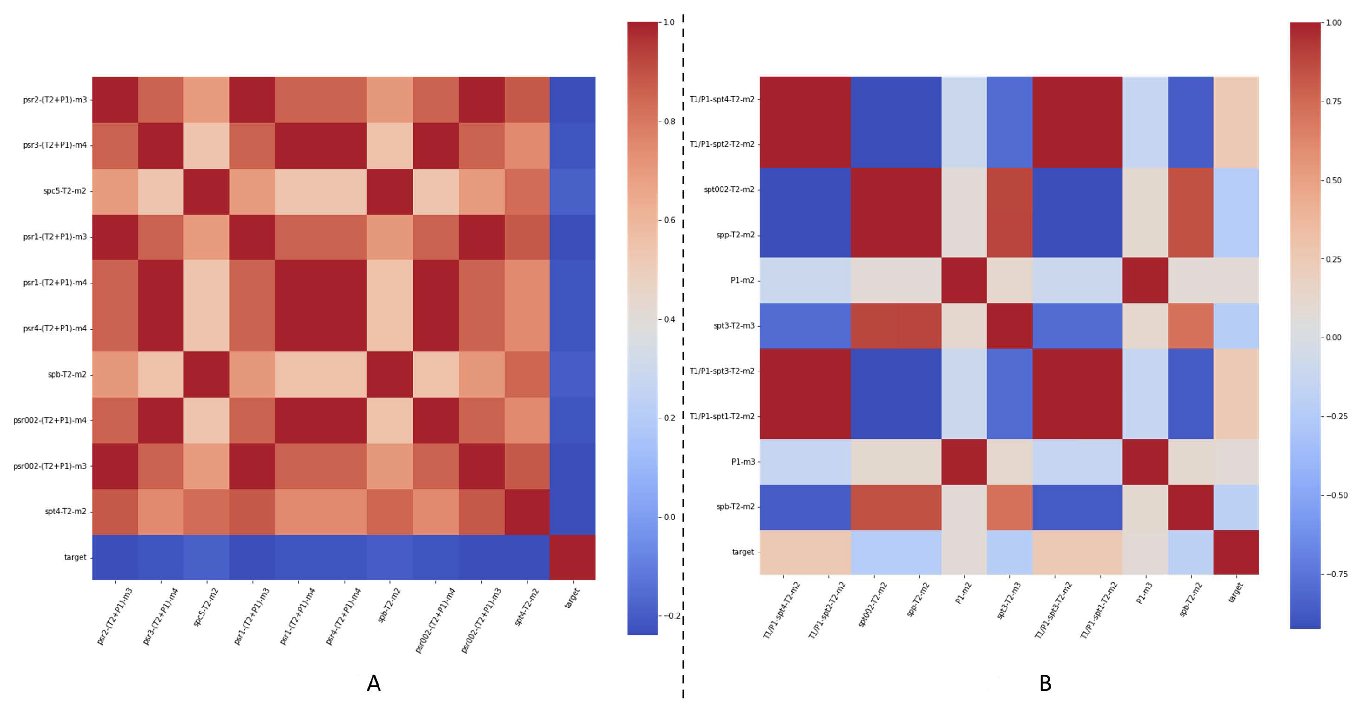
We created a total of 198 features. To avoid overfitting the machine learning models, we selected only K features, obtaining K from $\sqrt{N}$, where N is the number of instances in the training subset, as suggested by [82]. Feature selection was performed by computing their mutual information [83], and selecting the top K most informative ones. We describe the correlation between the selected features and target C5 content values we aim to forecast in Figure 5, Figure 6 and Figure 7.

4.4. Machine-Learning Model Development

4.4.1. Regression Machine Learning Models

Forecasting LPG C5 content solely from temperature and pressure data is a challenging task. In Figure 8, C5 content could reach very disparate values: from values close to zero to a range of valid values when considering the LPG specifications, and some peaks corresponding to samples with C5 concentrations well above the specification ranges. In our research, we developed and compared six models. These models include two baseline models and four models that aim to provide enhanced forecasts, and which we describe below:

• Baseline 1 (C5 median): our prediction is the median of C5 values observed in the data set for model training;
• Baseline 2 (LiR): linear regression to predict C5 content based on raw temperature and pressure sensor measurements (P1 and T2 from Figure 1, described in Feature Group ID #1 at Table 3);
• Model 1 (LiR): linear regression considering raw sensor measurements of P1 and T2 sensors at fifteen-minute intervals (see Figure 1, and all features described in Table 3), for the time range as presented in Figure 3;
• Model 2 (SVR): Support Vector Regressor [84], which takes into account most relevant features assessed over all created features;
• Model 3 (MLPR): Multi-layer Perceptron regressor [85], which takes into account most relevant features assessed over all created features;
• Model 4 (VR): composite model introduced in Figure 9, and described in detail later in this section. The model takes into account most relevant features assessed over all created features.

We expect that most of the time, C5 content levels remain within a threshold. Thus, predicting the median of C5 content observed in the past (Baseline 1) provides a realistic estimate that is not sensitive to outliers. Furthermore, we expect good machine learning models to surpass such a baseline, showing they learned patterns that allow more precise forecasts. Although the Baseline 2 (LiR) is a linear regression model that forecasts C5 content based only on raw temperature and pressure readings obtained from two sensors, Model 1 (LiR) provides insights on how the forecasting quality is improved by introducing a more extensive set of features (all features presented in Table 3), considering Roult’s law and Antoine’s equations, given the assumptions and simplifications described in Section 4.3. Model 2 (SVR) and Model 3 (MLPR) were built based on the SVR and MLPR algorithms, which were frequently reported in the related work. We instantiated the Model 2 (SVR) model with a radial basis function kernel, using an epsilon value of 0.1 and non-scaled L2 regularization. We did not impose constraints on the number of iterations required by the solver. Model 3 (MLPR) was instantiated with a single hidden layer of a hundred neurons, using a ReLU activation [86] and the Adam solver [87]. The learning rate was set to a fixed constant (0.001), and we trained it for 300 iterations. A validation set was created randomly sampling 0.1 of the training set.

We designed Model 4 (VR) (see Figure 9) as a voting regressor (VR) [88] that takes the input from four estimators to decide on the final forecast. Two estimators are CatBoost [89] models ((A) and (B)), each of them optimized with a different metrics function. (A) is optimized for the Root Mean Square Error (RMSE) metric, which tends to give more weight to points further away from the mean, and thus focuses on better adjusting off-specification values. On the other side, (B) is optimized for the Mean Absolute Error (MAE), which is not sensitive to outliers and ends up providing better estimates on the usual C5 levels. For both models, we use the expectile loss [90], which places unequal weights on disturbances. The expectile level (α) represents the center of mass of a probability distribution. The probabilities to the right are measured with α, while the probabilities to the left are measured with 1 − α [91]. Providing an asymmetric penalization of errors for the scored instances emphasizes instances whose output was not properly learned and yielded a greater forecast error. Both estimators are fed to the voting regressor, which issues a final forecast.

It is important to highlight that though C5 content data are available from laboratory analysis, we avoid using features based on past C5 measurements to ensure that the final model can load the sensor data and provide real-time C5 content estimates.

4.4.2. Classification Machine Learning Models

Forecasting if C5 content is off specification is a challenging task given the strongly imbalanced data. Only 14 out of 167 measurements in Unit A corresponded to such events in our particular use case, while no such events were registered in Unit B. In our research, we compared six models; two baseline models and four models that aim to provide better predictions:

• Baseline 1 (zero forecast): we predict no off-spec occurrence takes place;
• Baseline 2 (LgR): logistic regression to predict C5 content based on raw temperature and pressure sensor measurements (P1 and T2 from Figure 1, described in Feature Group ID #1 at Table 3);
• Model 1 (LgR): logistic regression considering raw sensor measurements of P1 and T2 sensors at fifteen-minute intervals (see Figure 1), and all features described in Table 3, for the time range as presented in Figure 3;
• Model 2 (SVC): Support Vector Classifier [84], which takes into account most relevant features assessed over all created features;
• Model 3 (MLPC): Multi-layer Perceptron Classifier [85], which takes into account most relevant features assessed over all created features;
• Model 4 (CatBoost): a CatBoost classifier with a Focal loss [92], which provides an asymmetric penalization to training instances, focusing more on those that are misclassified. The model takes into account most relevant features assessed over all created features.

We expect that most of the time, C5 content levels remain within the required specifications. Thus, predicting that no off-spec event takes place (Baseline 1) provides a realistic estimate that is accurate in all cases, except for a handful of cases where such an anomaly takes place. We expect the machine learning models to surpass such a baseline, showing they can accurately predict off-spec events, without introducing many false positives and negatives. The Baseline 2 (LgR) and Model 1 (LgR) were initialized with the same parameters, using a limited-memory Broyden–Fletcher–Goldfarb–Shannon solver algorithm [93,94,95,96], along with a L2 regularization. In both cases, a class balancing strategy was used to weights classes inversely proportional to class frequencies. Model 2 (SVC) was initialized with a radial basis function kernel and epsilon value of 0.1 and L2 regularization. We did not constrain the number of solver iterations. We initialized the Model 3 (MLPC) with a single hidden layer of a hundred neurons, with a ReLU activation and Adam solver. We used a constant learning rate (0.001) and trained the model over 300 iterations, with a validation set obtained by random sampling 0.1 of the training set. Finally, the CatBoost model was initialized with a Focal loss, growing asymmetric trees, a depth of six nodes, and a maximum number of 64 leaves. We trained the model over a thousand iterations, with a learning rate of 0.0299 evaluating against the AUC ROC metric. In all cases, we standardized features by removing the mean and scaling them to unit variance.

When building the classification models, we avoided using features based on past C5 measurements to ensure the models consume only data that can be provided in real time, and thus issue real-time forecasts.

5. Experiments and Results

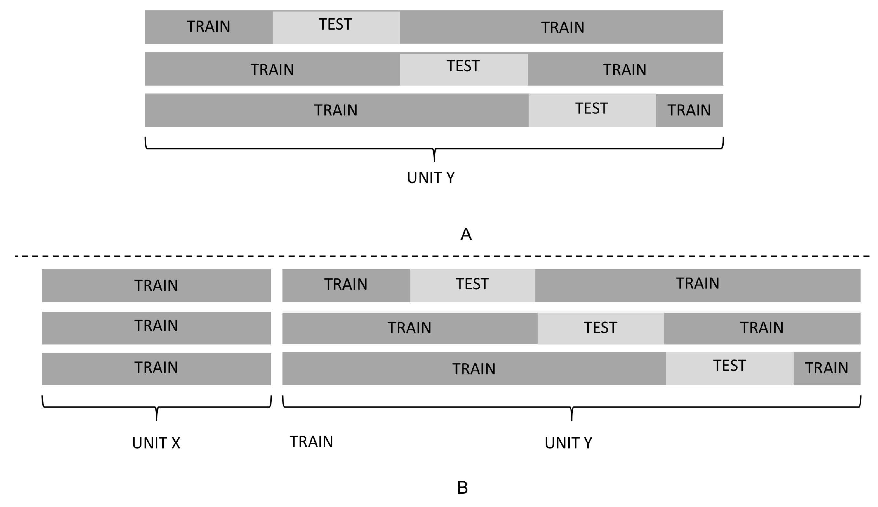
To evaluate the models presented in Section 4.4, we ran a repeated ten-fold cross-validation [97], executing 50 cross-validation runs. We conducted four experiments: two for regression models and two for classification models. Either for regression and classification, the experiments consisted of training the model only with historical data of the debutanizer unit we aim to predict for (Experiment 1), and to enrich the model validation with the data available from another debutanizer unit (Experiment 2). We present the corresponding cross-validation setting in Figure 10. We ensure results from both experiments are comparable by preserving the same cross-validation test sets among both experiments. We also assessed if the differences in results obtained for the different models were statistically significant. To that end, we executed the Wilcoxon signed-rank test [98] and tested for significance at a 95% level.

5.1. Regression Models

When implementing the experiments for the regression models presented in Section 4.4.1, we measured MAE and RMSE metrics. We present the results in

Table 4. Experiment 1 results. Mean RMSE and MAE values we obtained for different models with a ten-fold cross-validation, repeated 50 times. Best results are bolded, second-best are reported in italics. The results within the same column, which have no statistically significant difference between them when tested with a Wilcoxon paired rank test at a 95% confidence level, are marked with * and **.

Model	Unit A		Unit B
	RMSEmean	MAEmean	RMSEmean	MAEmean
Baseline 1 (C5 median)	** 1.1179	* 0.6028	0.1174	* 0.0853
Baseline 2 (LR)	** 1.1794	0.7601	1.4150	0.7248
Model 1 (LR)	1632.9693	560.4650	96826.5563	46730.6566
Model 2 (SVR)	* 1.0754	* 0.6087	* 0.1240	0.0991
Model 3 (MLPR)	* 1.0728	0.7122	0.2115	0.1424
Model 4	1.0352	* 0.6127	* 0.1201	* 0.0871

and

Table 5. Experiment 2 results. Mean RMSE and MAE values we obtained for different models with a ten-fold cross-validation, repeated 50 times. Best results are bolded, second-best are reported in italics. The results within the same column, which have no statistically significant difference between them when tested with a Wilcoxon paired rank test at a 95% confidence level, are marked with * and **. The arrows indicate whether the mean result improved (↑), or degraded (↓) when compared to Experiment 1.

Model	Unit A		Unit B
	RMSEmean	MAEmean	RMSEmean	MAEmean
Baseline 1 (C5 median)	1.1760↓	0.6141↓	0.1152↑	0.0818↑
Baseline 2 (LR)	1.0603↑	0.7009↑	** 0.2126↑	0.1978↑
Model 1 (LR)	1198266158.9503↓	411001902.3054↓	** 0.2753↑	0.1900↑
Model 2 (SVR)	1.1098↓	0.6193↓	* 0.1287↓	0.1021↓
Model 3 (MLPR)	1.0771↓	0.7234↓	0.2044↑	0.1581↓
Model 4	0.9655↑	0.5743↑	* 0.1270↓	0.0852↑

. From Experiment 1, we observed the best overall performance was achieved with Model 4 (VR), which demonstrates the best performance for all the scenarios except for one (RMSE for Unit B), where it achieved the second-best prediction. This performance was nearly matched by Baseline 1 (C5 median), which achieved the best performance in three cases: Unit B, and MAE for Unit A. We consider the Model 2 (SVR) was the third-best model among the evaluated ones, achieving the second-best prediction in all cases, except for MAE at Unit A, where it matched the best performance displayed by Model 4 (VR) and Baseline 1 (C5 median). Moreover, we found the Model 1 (LiR) demonstrated a significantly worse performance, which we attribute to the feature selection. We ground this conclusion on the fact that a better result was obtained by Baseline (LiR), and while some improvement was observed when augmenting the data in Experiment 2, it did not match the performance of the rest of the models. The best overall performance for Experiment 2 was achieved by Model 4 (VR), which achieved the best performance at Unit A, and second-best for Unit B. We consider the overall second-best performance was achieved by Baseline 1 (C5 median), which had the best performance in Unit B, and second-best considering MAE at Unit A.

When comparing results from both experiments, we observed Model 4 (VR) displayed the best performance, surpassing the Baseline 1 (C5 median). Model 4 (VR) is used to predict the C5 peaks providing good forecasts for low C5 levels, which reflects on the close results when compared to Baseline 1 (C5 median). Although the SVR algorithm is frequently reported in the literature, it achieved the third-best performance in Experiment 1 and degraded in Experiment 2. Using data from both units to train the models improved the performance of Baseline 2 (LiR) and Model 4 (VR) in all cases. It also improved the performance of Model 1 (LiR) for Unit B, and degraded the performance of Model 3 (MLPR) in all cases, except when measuring RMSE for Unit B.

Finally, we assessed which features were considered most informative by the feature selection criteria for both experiments. We found that from Experiment 1, the most relevant features were the pressure sensor readings, features from Feature Group 6 (ratio between expected T1 temperature and P1 pressure, for the given LPG mixtures—see Table 3), and categorical features indicating whether the pressure sensor readings are below 7.14 kg/cm², or above 7.63 kg/cm². However, the set of relevant features in Experiment 2 changed. Among the most important ones, we found those from Feature Group 2 (expected mixture saturation vapor pressure for considering temperature T2—see Table 3), and those from Feature Group 6. Pressure measures were still considered relevant in Experiment 2, but their importance faded in the presence of the ones mentioned above.

5.2. Classification Models

When implementing the experiments for the classification models presented in Section 4.4.2, we measured the AUC ROC metric. From

Table 6. Out-of-specification detection results for Unit A. Mean ROC AUC values we obtained for different models with a ten-fold cross-validation, repeated 50 times. Best results are bolded, second-best are reported in italics. The results within the same column, which have no statistically significant difference between them when tested with a Wilcoxon paired rank test at a 95% confidence level, are marked with *. The arrows indicate whether the mean result improved (↑), or degraded (↓) when compared to Experiment 1. Unit B is not reported, since the dataset did not include out-of-spec measurements for Unit B.

Model	Experiment 1	Experiment 2
	AUC ROCmean	AUC ROCmean
Baseline 1 (zero forecast)	0.5000	* 0.5000
Baseline 2 (LR)	0.5656	↑0.5675
Model 1 (LR)	0.6567	↓0.6059
Model 2 (SVC)	0.4491	* ↑0.4897
Model 3 (MLPC)	0.6709	↓0.5381
Model 4 (Catboost)	0.7359	↑0.7670

, we found that the best classification performance was obtained by Model 4 (CatBoost) in both experiments, with an AUC ROC of at least 0.7359, and surpassing the second-best model by 0.065 points in the worst case. However, best results were achieved in Experiment 2.

The second-best model in Experiment 1 was the Model 2 (MLPC), and the Model 1 (LgR) for Experiment 2. When comparing the model performance across experiments, we observed an increased performance in Experiment 2 for the Baseline 2 (LR) and Model 2 (SVC) models. On the other hand, a decreased discrimination power was measured for Model 1 (LgR), and Model 3 (MLPC). Model 2 (SVC) performed worse than a zero forecast in both experiments, but this difference was not statistically significant in Experiment 2. We hypothesize that the performance decrease in Experiment 2 for certain models can be related to the stronger class imbalance (8% event occurrence in Experiment 1 is reduced to 5% event occurrence in Experiment 2). Such imbalance influences the learning of the algorithms, and most likely affects the discrimination power of the trained models. We found the differences between results within the experiments were statistically significant, except between the Baseline 1 (zero forecast) and Model 2 (SVC) in Experiment 2.

Finally, we analyzed which features were considered most informative under the mutual information criteria for each experiment. For Experiment 1 the most informative features were the readings from the pressure sensor, categorical features indicating whether the sensed pressure is below 7.14 kg/cm², or below 7.06 kg/cm², and features from Features Group 4 (see Table 3). This changed for Experiment 2, where the most important features were related to readings from the pressure sensor and the Features Group 5.

5.3. Explaining Artificial Intelligence Models

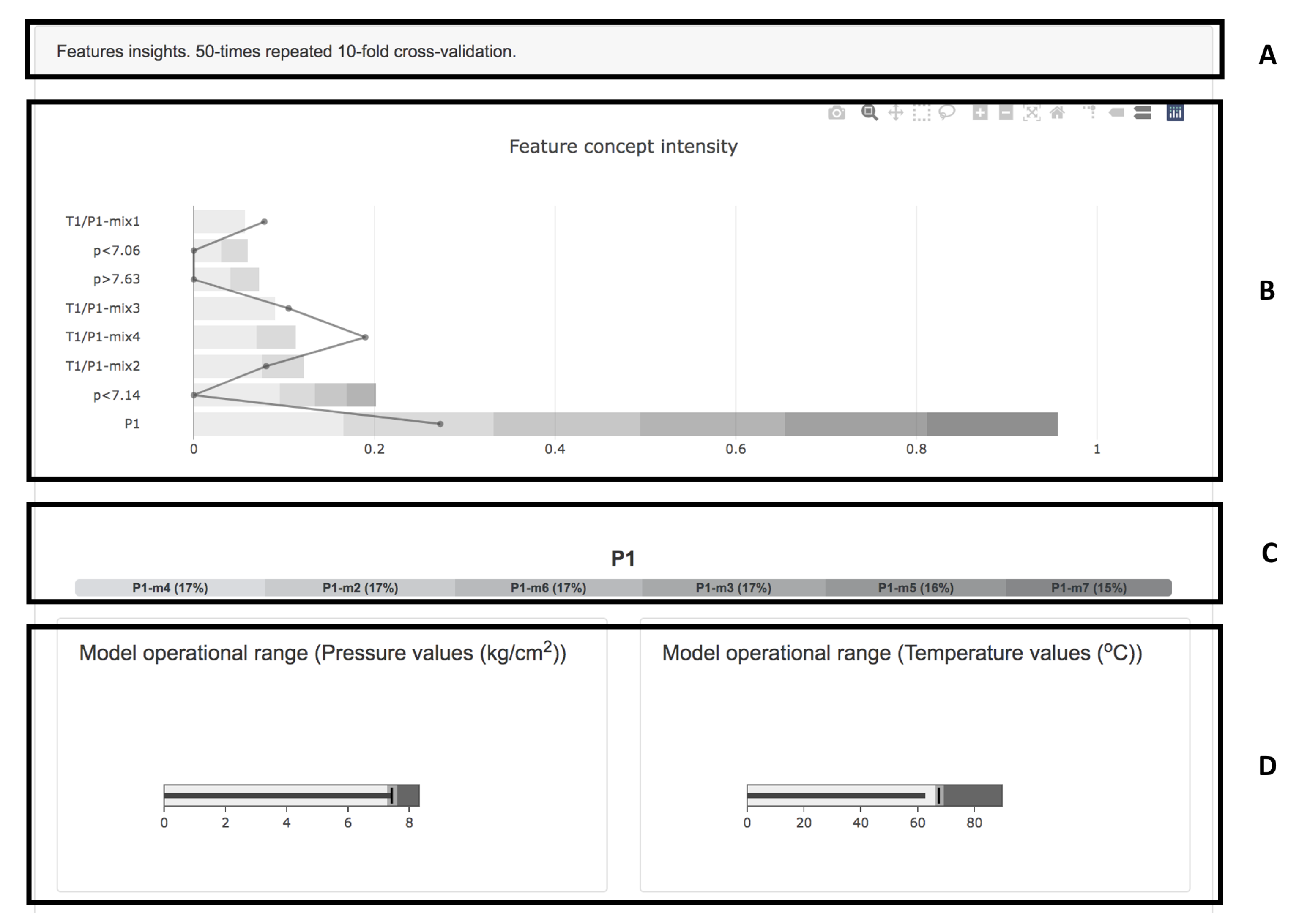
Although model accuracy is of great importance, insights on model rationale are required to assess the main factors driving the forecast are reasonable, and thus the forecast can be trusted. Although much research in the literature was devoted to global explanations, we found few authors taking into account the data or model training process. Furthermore, we found no authors combined insights regarding feature selection, and how relevant the selected features are to the model across a repeated cross-validation. We therefore propose a novel visualization that summarizes the aforementioned insights (see Figure 11).

Although much research work in the literature has been devoted to global explanations, and some related work focuses on the characteristics of the dataset, little research has been done on integrating insights regarding the dataset, the experimental setting, and the resulting model. We therefore propose a novel visualization which combines the three aforementioned parts. Figure 11A provides a brief description regarding the experimental setting. In this particular case, it states that the corresponding plots result from data obtained when training a forecasting model in a repeated 10-fold cross-validation setting, repeating the cross-validation 50 times. Figure 11B shows a horizontal stacked bar plot, where the intensity of feature concepts is presented to the users. We consider feature concepts as semantic abstractions that group certain features based on feature metadata. In our particular case, such grouping was performed for features computed with the same formula, but using sensor data at different points in time (see Figure 3). The shades of gray within the horizontal stacked bars represent how frequently was each feature of the feature concepts abstraction chosen when performing feature selection, within the 50 times 10-fold cross-validation. The line chart overlayed to the horizontal stacked bar plot informs how relevant were those feature concepts to the forecasting machine learning models, on average. Such overlay provides useful information to the machine-learning engineer, who can remove features found not informative to the model, to give room to better ones. In this particular case, we found three such cases ($p<7.06$, $p>7.63$, and $p<7.14$), referring to features with Boolean values, assessing whether the pressure values obtained from the sensor were above or below certain threshold value. By clicking a particular feature concept in the horizontal bar stacked plot, the section highlighted in Figure 11C is updated. Figure 11C enriches the aforementioned view, detailing each feature’s relevance within the specific feature concept. Finally, the bullet charts in Figure 11D provide insights into the values distribution for both sensors (P1 and T2). We explain the bullet chart with greater detail in Figure 12. The bullet chart has three segments, corresponding to quartiles Q1, Q2 + Q3, and Q4. A vertical bar in the Q2 + Q3 marks the median value, while a dark horizontal bar within the bullet chart, shows the mean value observed in the readings.

6. Conclusions

In this paper, two machine learning models are developed to forecast the concentration of pentanes (C5) in the LPG debutanization process. The first one is a regression model that provides pentane concentration estimates. The second one is a classifier that predicts whether the pentane concentration levels exceed allowed thresholds. Both models were designed to provide real-time forecasts based on sensor data. The advantages of the models are that only two sensors are required (temperature and pressure sensors, located at two distinct points at the top of the debutanizer column). Both models were compared against several baseline models, and machine learning models developed based on algorithms cited in the literature.

Our experiments show that the best results for the pentanes concentration estimation was obtained with a voting regressor, trained with historical data of the debutanizer unit. The model surpasses the performance achieved by a baseline predicting the pentane concentration as a median of past values and a linear regressor predicting the concentration from raw sensor values. When predicting the off-specification detection, best results were achieved with a CatBoost classifier trained with a focal loss over the data of both debutanizer units considered in this research. The model achieved an AUC ROC of 0.7670. In both cases, the addition of data from another debutanizer unit boosted the learning and consequent performance of most of the models.

In addition to the aforementioned models, we developed a prototype dashboard that allows visualization of relevant information regarding feature selection, features relevance to the model, and sensor reading values within which the model was trained. Such a dashboard is useful to assess strengths, limitations and improvement opportunities regarding the developed models.

We envision several directions for future research. First, we would like to extend these experiments to a broader range of debutanizer units. Secondly, we would like to compare the current approach to more complex settings, where a broader range of sensors is available. Finally, we consider that this approach can be applied in other industries using distillation processes and where soft sensors predicting specific substance concentrations are helpful.

References

1. Bradley, A.P. The use of the area under the ROC curve in the evaluation of machine learning algorithms. Pattern Recognit. 1997, 30, 1145–1159. [Google Scholar] [CrossRef] [Green Version]
2. Ferrer-Nadal, S.; Yélamos-Ruiz, I.; Graells, M.; Puigjaner, L. On-line fault diagnosis support for real time evolution applied to multi-component distillation. In Proceedings of the European Symposium on Computer-Aided Process Engineering-15, 38th European Symposium of the Working Party on Computer Aided Process Engineering, Barcelona, Spain, 29 May–1 June; Puigjaner, L., Espuña, A., Eds.; Elsevier: Amsterdam, The Netherlands, 2005; Volume 20, pp. 961–966. [Google Scholar] [CrossRef]
3. Abdullah, Z.; Aziz, N.; Ahmad, Z. Nonlinear Modelling Application in Distillation Column. Chem. Prod. Process. Model. 2007, 2. [Google Scholar] [CrossRef]
4. Michelsen, F.A.; Foss, B.A. A comprehensive mechanistic model of a continuous Kamyr digester. Appl. Math. Model. 1996, 20, 523–533. [Google Scholar] [CrossRef]
5. Franzoi, R.E.; Menezes, B.C.; Kelly, J.D.; Gut, J.A.; Grossmann, I.E. Cutpoint Temperature Surrogate Modeling for Distillation Yields and Properties. Ind. Eng. Chem. Res. 2020, 59, 18616–18628. [Google Scholar] [CrossRef]
6. Friedman, Y.; Neto, E.; Porfirio, C. First-principles distillation inference models for product quality prediction. Hydrocarb. Process. 2002, 81, 53–60. [Google Scholar]
7. Garcia, A.; Loria, J.; Marin, A.; Quiroz, A. Simple multicomponent batch distillation procedure with a variable reflux policy. Braz. J. Chem. Eng. 2014, 31, 531–542. [Google Scholar] [CrossRef]
8. Ryu, J.; Maravelias, C.T. Computationally efficient optimization models for preliminary distillation column design and separation energy targeting. Comput. Chem. Eng. 2020, 143, 107072. [Google Scholar] [CrossRef]
9. Küsel, R.R.; Wiid, A.J.; Craig, I.K. Soft sensor design for the optimisation of parallel debutaniser columns: An industrial case study. IFAC-PapersOnLine 2020, 53, 11716–11721. [Google Scholar] [CrossRef]
10. Ibrahim, D.; Jobson, M.; Guillen-Gosalbez, G. Optimization-based design of crude oil distillation units using rigorous simulation models. Ind. Eng. Chem. Res. 2017, 56, 6728–6740. [Google Scholar] [CrossRef] [Green Version]
11. Schäfer, P.; Caspari, A.; Schweidtmann, A.M.; Vaupel, Y.; Mhamdi, A.; Mitsos, A. The Potential of Hybrid Mechanistic/Data-Driven Approaches for Reduced Dynamic Modeling: Application to Distillation Columns. Chem. Ing. Tech. 2020, 92, 1910–1920. [Google Scholar] [CrossRef]
12. Bachnas, A.; Tóth, R.; Ludlage, J.; Mesbah, A. A review on data-driven linear parameter-varying modeling approaches: A high-purity distillation column case study. J. Process. Control 2014, 24, 272–285. [Google Scholar] [CrossRef] [Green Version]
13. Eikens, B.; Karim, M.N.; Simon, L. Neural Networks and First Principle Models for Bioprocesses. IFAC Proc. Vol. 1999, 32, 6974–6979. [Google Scholar] [CrossRef]
14. McBride, K.; Sanchez Medina, E.I.; Sundmacher, K. Hybrid Semi-parametric Modeling in Separation Processes: A Review. Chem. Ing. Tech. 2020, 92, 842–855. [Google Scholar] [CrossRef]
15. Schweidtmann, A.M.; Bongartz, D.; Huster, W.R.; Mitsos, A. Deterministic global process optimization: Flash calculations via artificial neural networks. In Computer Aided Chemical Engineering; Elsevier: Amsterdam, The Netherlands, 2019; Volume 46, pp. 937–942. [Google Scholar]
16. van Lith, P.F.; Betlem, B.H.; Roffel, B. Combining prior knowledge with data driven modeling of a batch distillation column including start-up. Comput. Chem. Eng. 2003, 27, 1021–1030. [Google Scholar] [CrossRef] [Green Version]
17. Chen, L.; Hontoir, Y.; Huang, D.; Zhang, J.; Morris, A. Combining first principles with black-box techniques for reaction systems. Control. Eng. Pract. 2004, 12, 819–826. [Google Scholar] [CrossRef]
18. Cubillos, F.; Callejas, H.; Lima, E.; Vega, M. Adaptive control using a hybrid-neural model: Application to a polymerisation reactor. Braz. J. Chem. Eng. 2001, 18, 113–120. [Google Scholar] [CrossRef]
19. Chang, J.S.; Lu, S.C.; Chiu, Y.L. Dynamic modeling of batch polymerization reactors via the hybrid neural-network rate-function approach. Chem. Eng. J. 2007, 130, 19–28. [Google Scholar] [CrossRef]
20. Siddharth, K.; Pathak, A.; Pani, A. Real-time quality monitoring in debutanizer column with regression tree and ANFIS. J. Ind. Eng. Int. 2018, 15, 41–51. [Google Scholar] [CrossRef] [Green Version]
21. Ochoa-Estopier, L.M.; Jobson, M. Optimization of Heat-Integrated Crude Oil Distillation Systems. Part I: The Distillation Model. Ind. Eng. Chem. Res. 2015, 54, 4988–5000. [Google Scholar] [CrossRef]
22. Shang, C.; Yang, F.; Huang, D.; Lyu, W. Data-driven soft sensor development based on deep learning technique. J. Process. Control 2014, 24, 223–233. [Google Scholar] [CrossRef]
23. Michalopoulos, J.; Papadokonstadakis, S.; Arampatzis, G.; Lygeros, A. Modelling of an Industrial Fluid Catalytic Cracking Unit Using Neural Networks. Chem. Eng. Res. Des. 2001, 79, 137–142. [Google Scholar] [CrossRef]
24. Bollas, G.; Papadokonstadakis, S.; Michalopoulos, J.; Arampatzis, G.; Lappas, A.; Vasalos, I.; Lygeros, A. Using hybrid neural networks in scaling up an FCC model from a pilot plant to an industrial unit. Chem. Eng. Process. Process. Intensif. 2003, 42, 697–713. [Google Scholar] [CrossRef]
25. Fortuna, L.; Graziani, S.; Xibilia, M. Soft sensors for product quality monitoring in debutanizer distillation columns. Control. Eng. Pract. 2005, 13, 499–508. [Google Scholar] [CrossRef]
26. Pani, A.K.; Amin, K.G.; Mohanta, H.K. Soft sensing of product quality in the debutanizer column with principal component analysis and feed-forward artificial neural network. Alex. Eng. J. 2016, 55, 1667–1674. [Google Scholar] [CrossRef] [Green Version]
27. Ge, Z.; Song, Z. A comparative study of just-in-time-learning based methods for online soft sensor modeling. Chemom. Intell. Lab. Syst. 2010, 104, 306–317. [Google Scholar] [CrossRef]
28. Zheng, J.; Song, Z.; Ge, Z. Probabilistic learning of partial least squares regression model: Theory and industrial applications. Chemom. Intell. Lab. Syst. 2016, 158, 80–90. [Google Scholar] [CrossRef]
29. Ge, Z. Active learning strategy for smart soft sensor development under a small number of labeled data samples. J. Process. Control 2014, 24, 1454–1461. [Google Scholar] [CrossRef]
30. Ge, Z. Supervised Latent Factor Analysis for Process Data Regression Modeling and Soft Sensor Application. IEEE Trans. Control Syst. Technol. 2016, 24, 1004–1011. [Google Scholar] [CrossRef]
31. Yao, L.; Ge, Z. Locally Weighted Prediction Methods for Latent Factor Analysis with Supervised and Semisupervised Process Data. IEEE Trans. Autom. Sci. Eng. 2017, 14, 126–138. [Google Scholar] [CrossRef]
32. Yuan, X.; Ye, L.; Bao, L.; Ge, Z.; Song, Z. Nonlinear feature extraction for soft sensor modeling based on weighted probabilistic PCA. Chemom. Intell. Lab. Syst. 2015, 147, 167–175. [Google Scholar] [CrossRef]
33. Bidar, B.; Sadeghi, J.; Shahraki, F.; Khalilipour, M.M. Data-driven soft sensor approach for online quality prediction using state dependent parameter models. Chemom. Intell. Lab. Syst. 2017, 162, 130–141. [Google Scholar] [CrossRef]
34. Mohamed Ramli, N.; Hussain, M.; Mohamed Jan, B.; Abdullah, B. Composition Prediction of a Debutanizer Column using Equation Based Artificial Neural Network Model. Neurocomputing 2014, 131, 59–76. [Google Scholar] [CrossRef]
35. Subramanian, R.; Moar, R.R.; Singh, S. White-box Machine learning approaches to identify governing equations for overall dynamics of manufacturing systems: A case study on distillation column. Mach. Learn. Appl. 2021, 3, 100014. [Google Scholar] [CrossRef]
36. Shi, J.; Wan, J.; Yan, H.; Suo, H. A survey of cyber-physical systems. In Proceedings of the 2011 International Conference on Wireless Communications and Signal Processing (WCSP), Nanjing, China, 9–11 November 2011; pp. 1–6. [Google Scholar]
37. Chen, H. Applications of cyber-physical system: A literature review. J. Ind. Integr. Manag. 2017, 2, 1750012. [Google Scholar] [CrossRef]
38. Lu, Y. Cyber physical system (CPS)-based industry 4.0: A survey. J. Ind. Integr. Manag. 2017, 2, 1750014. [Google Scholar] [CrossRef]
39. Khodabakhsh, A.; Ari, I.; Bakir, M.; Ercan, A.O. Multivariate Sensor Data Analysis for Oil Refineries and Multi-mode Identification of System Behavior in Real-time. IEEE Access 2018, 6, 64389–64405. [Google Scholar] [CrossRef]
40. Adadi, A.; Berrada, M. Peeking inside the black-box: A survey on explainable artificial intelligence (XAI). IEEE Access 2018, 6, 52138–52160. [Google Scholar] [CrossRef]
41. Keller, P.; Drake, A. Exclusivity and Paternalism in the public governance of explainable AI. Comput. Law Secur. Rev. 2021, 40, 105490. [Google Scholar] [CrossRef]
42. El-Assady, M.; Jentner, W.; Kehlbeck, R.; Schlegel, U.; Sevastjanova, R.; Sperrle, F.; Spinner, T.; Keim, D. Towards XAI: Structuring the Processes of Explanations. In Proceedings of the ACM Workshop on Human-Centered Machine Learning, Glasgow, UK, 4 May 2019. [Google Scholar]
43. Xu, F.; Uszkoreit, H.; Du, Y.; Fan, W.; Zhao, D.; Zhu, J. Explainable AI: A brief survey on history, research areas, approaches and challenges. In Proceedings of the CCF International Conference on Natural Language Processing and Chinese Computing, Gansu, China, 9–11 October 2019; Springer: Berlin/Heidelberg, Germany, 2019; pp. 563–574. [Google Scholar]
44. Arrieta, A.B.; Díaz-Rodríguez, N.; Del Ser, J.; Bennetot, A.; Tabik, S.; Barbado, A.; García, S.; Gil-López, S.; Molina, D.; Benjamins, R.; et al. Explainable Artificial Intelligence (XAI): Concepts, taxonomies, opportunities and challenges toward responsible AI. Inf. Fusion 2020, 58, 82–115. [Google Scholar] [CrossRef] [Green Version]
45. Loyola-Gonzalez, O. Black-box vs. white-box: Understanding their advantages and weaknesses from a practical point of view. IEEE Access 2019, 7, 154096–154113. [Google Scholar] [CrossRef]
46. Das, A.; Rad, P. Opportunities and challenges in explainable artificial intelligence (xai): A survey. arXiv 2020, arXiv:2006.11371. [Google Scholar]
47. Alicioglu, G.; Sun, B. A survey of visual analytics for Explainable Artificial Intelligence methods. Comput. Graph. 2021. [Google Scholar] [CrossRef]
48. Messalas, A.; Kanellopoulos, Y.; Makris, C. Model-agnostic interpretability with shapley values. In Proceedings of the 2019 10th International Conference on Information, Intelligence, Systems and Applications (IISA), Patras, Greece, 15–17 July 2019; pp. 1–7. [Google Scholar]
49. Frye, C.; de Mijolla, D.; Begley, T.; Cowton, L.; Stanley, M.; Feige, I. Shapley explainability on the data manifold. arXiv 2020, arXiv:2006.01272. [Google Scholar]
50. Polley, S.; Koparde, R.R.; Gowri, A.B.; Perera, M.; Nuernberger, A. Towards trustworthiness in the context of explainable search. In Proceedings of the 44th International ACM SIGIR Conference on Research and Development in Information Retrieval, Online, 11–15 July 2021; pp. 2580–2584. [Google Scholar]
51. Chan, G.Y.Y.; Bertini, E.; Nonato, L.G.; Barr, B.; Silva, C.T. Melody: Generating and Visualizing Machine Learning Model Summary to Understand Data and Classifiers Together. arXiv 2020, arXiv:2007.10614. [Google Scholar]
52. Chan, G.Y.Y.; Yuan, J.; Overton, K.; Barr, B.; Rees, K.; Nonato, L.G.; Bertini, E.; Silva, C.T. SUBPLEX: Towards a Better Understanding of Black Box Model Explanations at the Subpopulation Level. arXiv 2020, arXiv:2007.10609. [Google Scholar]
53. Krause, J.; Perer, A.; Bertini, E. INFUSE: Interactive feature selection for predictive modeling of high dimensional data. IEEE Trans. Vis. Comput. Graph. 2014, 20, 1614–1623. [Google Scholar] [CrossRef] [PubMed]
54. Seifert, C.; Aamir, A.; Balagopalan, A.; Jain, D.; Sharma, A.; Grottel, S.; Gumhold, S. Visualizations of deep neural networks in computer vision: A survey. In Transparent Data Mining for Big and Small Data; Springer: Berlin/Heidelberg, Germany, 2017; pp. 123–144. [Google Scholar]
55. Jin, W.; Carpendale, S.; Hamarneh, G.; Gromala, D. Bridging ai developers and end users: An end-user-centred explainable ai taxonomy and visual vocabularies. In Proceedings of the IEEE Visualization, Vancouver, BC, Canada, 20–25 October 2019; pp. 20–25. [Google Scholar]
56. Hudon, A.; Demazure, T.; Karran, A.; Léger, P.M.; Sénécal, S. Explainable Artificial Intelligence (XAI): How the Visualization of AI Predictions Affects User Cognitive Load and Confidence; Davis, F.D., Riedl, R., vom Brocke, J., Léger, P.-M., Randolph, A.B., Müller-Putz, G., Eds.; Springer: Cham, Switzerland, 2021; pp. 237–246. [Google Scholar]
57. Joia, P.; Coimbra, D.; Cuminato, J.A.; Paulovich, F.V.; Nonato, L.G. Local affine multidimensional projection. IEEE Trans. Vis. Comput. Graph. 2011, 17, 2563–2571. [Google Scholar] [CrossRef] [PubMed]
58. Wang, J.; Gou, L.; Zhang, W.; Yang, H.; Shen, H.W. Deepvid: Deep visual interpretation and diagnosis for image classifiers via knowledge distillation. IEEE Trans. Vis. Comput. Graph. 2019, 25, 2168–2180. [Google Scholar] [CrossRef] [PubMed]
59. Ribeiro, M.T.; Singh, S.; Guestrin, C. “Why should i trust you?” Explaining the predictions of any classifier. In Proceedings of the 22nd ACM SIGKDD International Conference on Knowledge Discovery and Data Mining, San Francisco, CA, USA, 13–17 August 2016; pp. 1135–1144. [Google Scholar]
60. Collaris, D.; van Wijk, J.J. ExplainExplore: Visual exploration of machine learning explanations. In Proceedings of the 2020 IEEE Pacific Visualization Symposium (PacificVis), Tianjin, China, 14–17 April 2020; pp. 26–35. [Google Scholar]
61. Ribeiro, M.T.; Singh, S.; Guestrin, C. Model-agnostic interpretability of machine learning. arXiv 2016, arXiv:1606.05386. [Google Scholar]
62. Alvarez-Melis, D.; Jaakkola, T.S. Towards robust interpretability with self-explaining neural networks. arXiv 2018, arXiv:1806.07538. [Google Scholar]
63. Viton, F.; Elbattah, M.; Guérin, J.L.; Dequen, G. Heatmaps for Visual Explainability of CNN-Based Predictions for Multivariate Time Series with Application to Healthcare. In Proceedings of the 2020 IEEE International Conference on Healthcare Informatics (ICHI), Oldenburg, Germany, 30 November–3 December 2020; pp. 1–8. [Google Scholar]
64. Rožanec, J.; Trajkova, E.; Kenda, K.; Fortuna, B.; Mladenić, D. Explaining Bad Forecasts in Global Time Series Models. Appl. Sci. 2021, 11, 9243. [Google Scholar] [CrossRef]
65. Greenwell, B.M. pdp: An R package for constructing partial dependence plots. R J. 2017, 9, 421. [Google Scholar] [CrossRef] [Green Version]
66. Apley, D.W.; Zhu, J. Visualizing the effects of predictor variables in black box supervised learning models. J. R. Stat. Soc. Ser. B (Stat. Methodol.) 2020, 82, 1059–1086. [Google Scholar] [CrossRef]
67. Council of the European Union; European Parliament. Regulation (EC) No 715/2007 of the European Parliament and of the Council; Technical report, 715/2007/EC; Official Journal of the European Union, Publications Office of the European Union: Luxembourg, 20 June 2007. [Google Scholar]
68. Luyben, W.L. Distillation column pressure selection. Sep. Purif. Technol. 2016, 168, 62–67. [Google Scholar] [CrossRef]
69. Liu, Z.Y.; Jobson, M. The effect of operating pressure on distillation column throughput. Comput. Chem. Eng. 1999, 23, S831–S834. [Google Scholar] [CrossRef]
70. Kister, H.Z. Distillation Operation; McGraw-Hill: New York, NY, USA, 1990. [Google Scholar]
71. Mejdell, T.; Skogestad, S. Composition estimator in a pilot-plant distillation column using multiple temperatures. Ind. Eng. Chem. Res. 1991, 30, 2555–2564. [Google Scholar] [CrossRef]
72. Huang, K.; Wang, S.J.; Iwakabe, K.; Shan, L.; Zhu, Q. Temperature control of an ideal heat-integrated distillation column (HIDiC). Chem. Eng. Sci. 2007, 62, 6486–6491. [Google Scholar] [CrossRef]
73. Behnasr, M.; Jazayeri-Rad, H. Robust data-driven soft sensor based on iteratively weighted least squares support vector regression optimized by the cuckoo optimization algorithm. J. Nat. Gas Sci. Eng. 2015, 22, 35–41. [Google Scholar] [CrossRef]
74. Aston, J.; Messerly, G. Additions and Corrections-The Heat Capacity and Entropy, Heats of Fusion and Vaporization, and the Vapor Pressure of n-Butane. J. Am. Chem. Soc. 1941, 63, 3549. [Google Scholar] [CrossRef]
75. Das, T.R.; Reed Jr, C.O.; Eubank, P.T. PVT [pressure-volume-temperature] surface and thermodynamic properties of butane. J. Chem. Eng. Data 1973, 18, 244–253. [Google Scholar] [CrossRef]
76. Carruth, G.F.; Kobayashi, R. Vapor pressure of normal paraffins ethane through n-decane from their triple points to about 10 mm mercury. J. Chem. Eng. Data 1973, 18, 115–126. [Google Scholar] [CrossRef]
77. Kemp, J.; Egan, C.J. Hindered rotation of the methyl groups in propane. The heat capacity, vapor pressure, heats of fusion and vaporization of propane. Entropy and density of the gas. J. Am. Chem. Soc. 1938, 60, 1521–1525. [Google Scholar] [CrossRef]
78. Rips, S. On a Feasible Level of Filling in of Reservoires by Liquid Hydrocarbons. Khim. Prom. (Moscow) 1963, 8, 610–613. [Google Scholar]
79. Helgeson, N.; Sage, B.H. Latent heat of vaporization of propane. J. Chem. Eng. Data 1967, 12, 47–49. [Google Scholar] [CrossRef]
80. Yaws, C.; Yang, H. To estimate vapor pressure easily. Hydrocarb. Process. (USA) 1989, 68. [Google Scholar]
81. Osborn, A.G.; Douslin, D.R. Vapor-pressure relations for 15 hydrocarbons. J. Chem. Eng. Data 1974, 19, 114–117. [Google Scholar] [CrossRef]
82. Hua, J.; Xiong, Z.; Lowey, J.; Suh, E.; Dougherty, E.R. Optimal number of features as a function of sample size for various classification rules. Bioinformatics 2005, 21, 1509–1515. [Google Scholar] [CrossRef] [Green Version]
83. Kraskov, A.; Stögbauer, H.; Grassberger, P. Estimating mutual information. Phys. Rev. E 2004, 69, 066138. [Google Scholar] [CrossRef] [PubMed] [Green Version]
84. Drucker, H.; Burges, C.J.; Kaufman, L.; Smola, A.; Vapnik, V. Support vector regression machines. Adv. Neural Inf. Process. Syst. 1997, 9, 155–161. [Google Scholar]
85. McCulloch, W.S.; Pitts, W. A logical calculus of the ideas immanent in nervous activity. Bull. Math. Biophys. 1943, 5, 115–133. [Google Scholar] [CrossRef]
86. Fukushima, K. Visual feature extraction by a multilayered network of analog threshold elements. IEEE Trans. Syst. Sci. Cybern. 1969, 5, 322–333. [Google Scholar] [CrossRef]
87. Kingma, D.P.; Ba, J. Adam: A method for stochastic optimization. arXiv 2014, arXiv:1412.6980. [Google Scholar]
88. An, K.; Meng, J. Voting-averaged combination method for regressor ensemble. In Proceedings of the International Conference on Intelligent Computing, Xiamen, China, 29–31 October 2010; Springer: Berlin/Heidelberg, Germany, 2010; pp. 540–546. [Google Scholar]
89. Dorogush, A.V.; Ershov, V.; Gulin, A. CatBoost: Gradient boosting with categorical features support. arXiv 2018, arXiv:1810.11363. [Google Scholar]
90. Aigner, D.; Lovell, C.K.; Schmidt, P. Formulation and estimation of stochastic frontier production function models. J. Econom. 1977, 6, 21–37. [Google Scholar] [CrossRef]
91. Ehm, W.; Gneiting, T.; Jordan, A.; Krüger, F. Of quantiles and expectiles: Consistent scoring functions, Choquet representations and forecast rankings. J. R. Stat. Soc. Ser. Stat. Methodol. 2016, 78 Pt 3, 505–562. [Google Scholar] [CrossRef] [Green Version]
92. Lin, T.Y.; Goyal, P.; Girshick, R.; He, K.; Dollár, P. Focal loss for dense object detection. In Proceedings of the IEEE International Conference on Computer Vision, Venice, Italy, 22–29 October 2017; pp. 2980–2988. [Google Scholar]
93. Broyden, C.G. The convergence of a class of double-rank minimization algorithms 1. general considerations. IMA J. Appl. Math. 1970, 6, 76–90. [Google Scholar] [CrossRef]
94. Fletcher, R. A new approach to variable metric algorithms. Comput. J. 1970, 13, 317–322. [Google Scholar] [CrossRef] [Green Version]
95. Goldfarb, D. A family of variable-metric methods derived by variational means. Math. Comput. 1970, 24, 23–26. [Google Scholar] [CrossRef]
96. Shanno, D.F. Conditioning of quasi-Newton methods for function minimization. Math. Comput. 1970, 24, 647–656. [Google Scholar] [CrossRef]
97. Stone, M. Cross-validatory choice and assessment of statistical predictions. J. R. Stat. Soc. Ser. B (Methodological) 1974, 36, 111–133. [Google Scholar] [CrossRef]
98. Wilcoxon, F. Individual comparisons by ranking methods. In Breakthroughs in Statistics; Springer: Berlin/Heidelberg, Germany, 1992; pp. 196–202. [Google Scholar]
Figure 1. High-level schematic diagram of some of units found in crude oil refineries. In this research we focus on one of the LPG debutanizer units.
Applsci 11 11790 g001
Figure 2. (A) shows a plot with three sample sensors timeseries. The dashed squares enclose some of the change levels observed in those time series. (B) shows two plots, related to the change level detector: on the top we observe the signal, and on the bottom the residual. If the residual exceeds certain threshold, a new interval is created.
Applsci 11 11790 g002
Figure 3. Timestamp conciliation between sensor and laboratory sample timestamps, based on insights provided by experts. Since a time range is provided, we decided to sample sensor values in the given interval every 15 minutes, adding a 15 minutes tolerance at the interval edges. Times provided in this example do not correspond to real timestamps in data.
Applsci 11 11790 g003
Figure 4. Schematic diagram of an LPG debutanizer column. In the diagram we reference two locations on which the sensors are placed. In this research, we developed models that take into account only sensors P1 and T2.
Applsci 11 11790 g004
Figure 5. Feature correlation for ten selected features in each case, when forecasting the amount of C5 present in distilled LPG at the end of the distillation process in the debutanizer columns, for Unit A. On (A) we present feature correlations for Experiment 1, while on (B) we present feature correlations for Experiment 2.
Applsci 11 11790 g005
Figure 6. Feature correlation for ten selected features in each case, when forecasting the amount of C5 present in distilled LPG at the end of the distillation process in the debutanizer columns, for Unit B. On (A) we present feature correlations for Experiment 1, while on (B) we present feature correlations for Experiment 2.
Applsci 11 11790 g006
Figure 7. Feature correlation for ten selected features in each case, when forecasting if the amount of C5 present in distilled LPG at the end of the distillation process in the debutanizer columns remains within the required specification thresholds, for Unit A. On (A) we present feature correlations for Experiment 1, while on (B) we present feature correlations when considering Experiment 2.
Applsci 11 11790 g007
Figure 8. Measured C5 content in laboratory samples over time. Please notice that the samples are taken at irregular intervals. On (A) we present measurements from Unit A, while on (B) we present measurements from Unit B.
Applsci 11 11790 g008
Figure 9. To estimate C5 content, we created a voting regressor that considers only sensor data as input. Regressors (A) and (B) correspond to CatBoost models with different optimization objectives: (A) optimizes against RMSE, penalizing large errors, while (B) optimizes against MAE to achieve best median performance. Outputs from models (A), and (B) are weighted by the voting regressor (C), to create the final forecast.
Applsci 11 11790 g009
Figure 10. We pose two experiments: Experiment 1 trains models only with data of the debutanizer unit we aim to predict for (A), while Experiment 2 enriches the training set with data from other debutanizer unit (B).
Applsci 11 11790 g010
Figure 11. The visualization summarizes relevant information regarding the dataset, and forecasting model: (A) describes the cross-validation setting, (B) informs most relevant feature concepts when considering feature selection and model features relevance, (C) details the weight of particular features within a feature concept, and (D) provides insights regarding values distribution for sensor data.
Applsci 11 11790 g011
Figure 12. The bullet chart summarizes the sensor values distribution: three segments, Q1, Q2 + Q3, and Q4 mark values related to the quartiles; a dark vertical bar within the Q2 + Q3 segment represents the median value, while the dark horizontal bar within the bullet chart informs the mean reading value.
Applsci 11 11790 g012