Abstract
To minimize the impacts of large losses and optimize the emergency response when a large earthquake occurs, an accurate early warning of an earthquake or tsunami is crucial. One important parameter that can provide an accurate early warning is the earthquake’s magnitude. This study proposes a method for estimating the magnitude, and some of the source parameters, of an earthquake using genetic algorithms (GAs). In this study, GAs were used to perform an inversion of Okada’s model from earthquake displacement data. In the first stage of the experiment, the GA was used to inverse the displacement calculated from the forward calculation in Okada’s model. The best performance of the GA was obtained by tuning the hyperparameters to obtain the most functional configuration. In the second stage, the inversion method was tested on GPS time series data from the 2011 Tohoku Oki earthquake. The earthquake’s displacement was first estimated from GPS time series data using a detection and estimation formula from previous research to calculate the permanent displacement value. The proposed method can estimate an earthquake’s magnitude and four source parameters (i.e., length, width, rake, and slip) close to the real values with reasonable accuracy.
1. Introduction
Earthquakes with large magnitudes always result in large losses and can even trigger a subsequent disaster such as a tsunami. To provide an early warning for tsunamis and facilitate emergency responses to earthquakes, one important parameter that needs to be known early and as accurately as possible is the earthquake’s magnitude [1]. Tsunami early warning systems in many countries such as Indonesia use the estimated magnitude of the earthquake as the main reference for providing tsunami early warnings [2,3]. If the earthquake’s magnitude is estimated at 6.5 or greater, the system will issue a warning that the earthquake has the potential to trigger a tsunami [3]. The tsunami potential of an earthquake must be decided within 3–5 min. However, the magnitude estimation performed by conventional estimation methods is far from accurate in such a short period of time. In some previous cases of large earthquakes that have triggered tsunamis, the early warning was inaccurate because the magnitude was underestimated at crucial times [4,5,6,7]. As a result, the earthquake’s impacts were larger than expected and caused a greater loss of life and infrastructure.
Conventionally, rapid magnitude estimation is still carried out based on seismometer data using magnitude scales that can be derived as soon as an earthquake occurs. Such scales include the body-wave magnitude (), surface-wave magnitude (), and moment magnitude () measurement scales [1]. However, these types of measurements have significant limitations when estimating values due to saturation problems hampering measurement equipment used to record seismic signals, especially in the event of a large earthquake. The signal amplitude is often clipped during major earthquakes. Stations nearest to the epicenter are the most important sources of information to obtain an early estimation of an earthquake’s magnitude. Unfortunately, these nearby stations are more susceptible to the saturation and clipping-off problems mentioned above, which can cause the magnitude to be underestimated compared with the actual value [4,5,7].
For example, in the 2004 Sumatran earthquake that triggered the most fatal tsunami in the country’s history, an initial estimate of the earthquake’s magnitude was released 11 min after the earthquake occurred: 8.0 using [1]. One hour after the earthquake occurred, the value was revised using to 8.5. The next update was given five hours after the earthquake, and the newly estimated magnitude was 9.0 [1]. The actual magnitude of 9.2 was ultimately released a few days later. The initial estimated value of magnitude (8.0) resulted in the tsunami early warning decision being underestimated, which led to a suboptimal emergency response. In the three hours after the earthquake occurred, a huge tsunami crossed the sea at high speed and devastated the nearby area [5,7].
When the Tohoku Oki earthquake occurred in 2011, the actual magnitude was similarly underestimated. This underestimation provided an inaccurate tsunami early warning followed by an emergency response that was far below the recommended standard. Three minutes after the earthquake occurred, the estimated magnitude released by the Japan Meteorology Agency was 7.9 [5]. This estimation was updated to 8.4 one hour and 20 min after the earthquake. A few days later, the actual magnitude was determined to be an of 9.0. In the 25 min after the earthquake occurred, a large tsunami destroyed the coast nearest to the source of the earthquake [5,7].
These two earthquake events show the importance of providing an accurate magnitude estimation within the crucial few minutes after the earthquake occurs [1,2,3,4,5,6,7,8]. However, because such estimation relies on seismic data from broadband seismometers and has not been able to address the saturation and clipping-off problems that occur after large earthquakes, alternative methodological approaches are needed to estimate an earthquake’s magnitude more accurately in a short space of time.
GPS, with its ability to record ground displacement data, has the potential to generate more accurate magnitude estimations without suffering saturation and clipping-off problems [6]. Indeed, some methods for rapid magnitude estimation based on GPS data have been examined in previous research [4,5,7,9,10,11,12,13,14]. This study proposes a method for rapidly estimating an earthquake’s magnitude based on an inversion of Okada’s model using a genetic algorithm (GA). This method can also estimate other source parameters such as the length, width, rake, and slip parameters of the fault plane.
GAs are optimization algorithms that can estimate many parameters to find the optimal value of an objective function [15]. Such algorithms are also known for their robustness in solving nonlinear problems [16,17]. In research on earthquake problems, GAs have been used to understand focal mechanisms and stress tensor inversion [18,19], carry out InSAR data inversion to learn about deformation [20], predict earthquakes [21], and select earthquake ground motion [22]. Other evolutionary computation-based algorithms have also been used to estimate the hypocenter location of an earthquake [23], inverse an earthquake’s dislocation [24], estimate earthquake magnitudes [25], estimate fault parameters [26,27], and solve engineering problems related to earthquakes [28].
In this study, the proposed rapid estimation method using GAs was tested on the 2011 Tohoku Oki earthquake data to measure its ability to estimate the earthquake’s source parameters and magnitude.
2. Materials and Methods
This study aimed to estimate earthquakes’ magnitudes and source parameters from GPS time series data recorded during an earthquake event. Here, the parameters were estimated using a GA to inverse the elastic dislocation equation based on Okada’s model. The hyperparameters of the GA were tuned to obtain the best configuration settings that yielded the best parameter estimation. The selected configuration was then tested on real displacement time series data from the GPS stations affected by the 2011 Tohoku Oki earthquake. GPS time series data from all stations were processed to estimate the permanent displacement value in both the horizontal and vertical components. The estimated permanent displacement was then inversed using the GA based on Okada’s model to obtain the source parameters.
2.1. Inversion of Okada’s Model
A fault is a large fracture in the Earth’s crust that causes two sides of rock blocks to become displaced relative to each other. An earthquake occurs due to a sudden release of energy that causes the fault to slip suddenly. The plane of the fracture where the fault slips is called the fault plane, and is represented by parameters such as strike, dip, depth, and rake [29]. Figure 1a illustrates a fault plane.
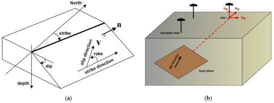
Figure 1.
Basic concepts related to elastic dislocation based on Okada’s model: (a) a fault plane with its parameters; (b) ground displacement as the effect of the slip of a fault plane.
A slip on the fault plane will cause some displacements on the seafloor of the Earth, which is called surface deformation. Okada’s elastic dislocation model, proposed by Okada in 1985, features a set of analytical solutions for surface displacements in a homogeneous half-space. This model translates the effect of a fault-plane slip into the ground displacements represented in [30], as illustrated in Figure 1b.
Okada’s model is widely used for co-seismic displacement analysis. The displacement field due to a dislocation across a surface in an isotropic medium is given by the following formula [31]:
A fault in an earthquake can be modeled as a collection of rectangular patches, where each patch has the following parameters [32]:
- The latitude and longitude of the fault plane’s centroid point;
- The length and width of the fault field (in meters or kilometers);
- The depth (in meters or kilometers);
- The strike (0–360°);
- The dip (0–90°);
- The rake (−180–180°);
- The slip (>0 m).
In simple terms, Okada’s model formulates these nine parameters to calculate the coseismic displacement fault values, tilts, and compression of an earthquake. This process can be expressed as a function of the nine parameters, which results in the following set of three-dimensional displacements [32]:
where and are the coordinates of the observation at the geographic reference (east and north) relative to the centroid of the fault plane, and is a set of displacement values at the observation points in the directions of north (), east (), and vertical (). Elastic dislocation modeling, in particular Okada’s model, requires the assumption of the fault plane’s centroid. In actual conditions, the centroid of an earthquake’s fault plane can be assumed to be the hypocenter location obtained from the seismic observations.
For the inversion of Okada’s model, a calculation in the inverse direction of the model is used to find some or all of the earthquake’s source parameters in the model function above from the displacement values at the observation points.
2.2. GAs
A GA is an optimization algorithm based on the principle of biological scientific selection. GAs are widely used in linear and nonlinear optimization problems [15,33,34]. In this study, the inversion of Okada’s model is also carried out through an optimization approach using GAs.
Based on Equation (2), the inversion process takes displacement data as the input to obtain the nine parameters of Okada’s model. However, this study only estimates four parameters through inversion: the length, width, rake, and slip parameters. The other parameters of , , depth, dip, and strike are predetermined parameters based on the earthquake fault model used in the experiment. GAs, as heuristic search algorithms, seek the best solutions for the estimated parameters.
In this study, the estimation results of the four variables along with the predetermined parameters are then used as input for the forward calculation of Okada’s model to obtain the displacement estimation values. There are two displacement values involved in this inversion process: actual displacement and estimated displacement. The actual displacement is calculated from GPS time series data using the permanent displacement formula, while the estimated displacement is obtained from the estimation using Okada’s model.
The generic GA is shown in Figure 2. The algorithm starts by initializing a population that consists of individuals representing solution candidates for the problem to be solved. The fitness of each candidate solution for the problem is then evaluated using an objective function called the fitness function. Two individuals with highest fitness score are then selected for the next parent candidate to produce new offspring through a crossover phase. The next step is the mutation phase to maintain or increase the genetic diversity of the population. This process will continue until the fitness value stabilizes and the algorithm has converged to an optimal solution. The following paragraphs provide more detailed descriptions about the implementation of each step in this study.
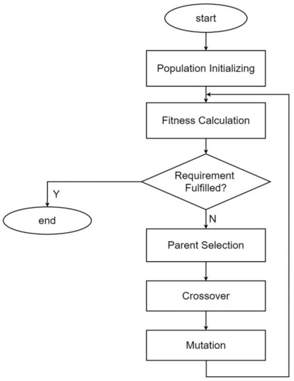
Figure 2.
Generic flowchart of a GA.
2.2.1. Population Initialization
The first step in this phase is to define individual representations as candidate solutions for the source parameter estimation problem. As mentioned previously, in this study the GA only estimates four parameters through the inversion, i.e., length, width, rake, and slip. Hence, in this study, each individual () consists of four chromosomes, , where is the chromosome representing the candidate solution for the th estimated variable, i.e., length, width, rake, and slip, respectively.
Each chromosome is represented as a number of bits. Therefore, the number of bits parameter () is tuned in this experiment. The number of bits will determine the number of possible values generated for each variable. Tuning of the number of bits parameter is described in the scenarios and settings section in Section 3.1. Each chromosome has a predetermined range of values that depends on the estimated variable it represents. According to the range of values for the Okada model parameters previously described in Section 2.1 and the parameter values of fault models tested, the search value for the length parameter ranges from 25 to 750 km, the width parameter from 10 to 300 km, the rake parameter from 60° to 120°, and the slip parameter from 0.1 to 25 m. The parameters of length, width, and rake are specified as integer data type, while the slip parameter is of real data type. The fault models tested in this study are described in detail in Section 3.1.1.
In addition to individual representation, another hyperparameter that needs to be determined in this phase is the size of the population, which denotes the number of individuals generated in one population. The size of the population is also included in the hyperparameter tuning of the experiment.
2.2.2. Fitness Calculation
The optimization problem in the source parameter estimation in this study is to find, for the four estimated variables, the optimal solutions that result in the minimum error value between the estimated displacement and the actual displacement. In other words, the closer the estimated displacement value is to the actual displacement value, the more optimal the model parameter estimation value is. Therefore, the objective function used in this study is the minimize function, and the minimized parameter is the error value between the estimated displacement and the actual displacement. The smaller the error value is, the more individuals that will be generated that will fit the optimal solution.
Error value representations used in the objective functions in this study are the mean square error (mse), square error (se), and the number of elements in the displacement matrix with a specific error value. Two objective functions were tested in the experiment to find the optimal estimation as follows:
where is the displacement error between the estimated displacement and actual or referred displacement; is the estimated displacement result from element data ; represents the referenced displacement value for element data , is the number of data points; and represents the number of elements for which the displacement errors are >1.
The estimated displacement () is obtained from the forward calculation of Okada’s model based on Equation (2) as follows:
where , , , , and are the predetermined parameters based on the earthquake’s fault model used in the calculation as described previously, while are the estimated variables of the source parameter length, width, rake, and slip, respectively. GA generates the estimation values for the estimated variables. The more optimal the estimation value for the variables, the more minimal the displacement error value will be. In other words, the estimated displacement () values are getting closer to the reference displacement () values.
Both objective functions in Equations (3) and (4) include the square error between estimated displacement and actual displacement, and the number of elements in the displacement matrix for which the displacement errors are >1. However, the second objective function also includes the mean square error of the displacements. Hence, the second objective function attempts to capture the central value of the displacement errors, in addition to accumulating the error values. One of the objective functions will be selected as the recommended optimal function based on the experimental results.
2.2.3. Parent Selection
The purpose of selecting parent candidates is to obtain better individuals or solution candidates than the previous generation. This study uses the tournament selection method to perform this selection. The selected parent candidate is the fittest individual among randomly chosen individuals in the population, with representing a predetermined hyperparameter in the tournament selection method. Individuals with the smallest error values will have the highest probability to be selected.
2.2.4. Crossover
The crossover method used in this study is one point crossover, which designates only one point to split the bit strings of the selected parents. Hence, each pair of selected parents will create two children. The splitting point is randomly selected in the experiment. The bit string representation of each created child refers to the bit string of its parents. The left part of the splitting point in the first child’s chromosomes refer to the first parent’s bit strings, and the right part of the splitting point refers to the second parent’s bit strings. The second child is created by inverting the process.
The crossover process is controlled by a parameter called crossover rate (, which denotes the probability of the crossover to be applied. Since the crossover concept is something that naturally occurs in real life, the crossover rate is generally set high.
2.2.5. Mutation
A mutation is used to maintain genetic variation within the population. Therefore, mutation is an important step to avoid a local minimum during the search for the optimum solution. Mutation involves bit flipping of the created child. The mutation rate denotes the probability of the mutation, which is typically low and set to where is the length of the bit strings representing the individual [35]. The formula for the mutation rate () is as follows [35]:
where denotes the number of bits in a chromosome, and is the number of chromosomes in an individual.
The set values for all GA hyperparameters used and tuned in this study are represented in the scenarios and setting subsection in Section 3. The inversion of Okada’s model using the GA will be referred to as the Okada–GA inversion model in this paper.
2.3. Moment Magnitude (Mw) Estimation
Moment is related to the total energy released during an earthquake event. Moment is proportional to the slip on the fault multiplied by the fault area that slips. The formula is shown below [36]:
where is moment seismicity, is the rigidity parameter or shear modulus of the crust (approximately ), is the fault length (m), is the fault width (m), and is the slip length (m).
Moment seismicity can be converted into an earthquake’s magnitude standard called moment magnitude using the following formula [36]:
2.4. Permanent Displacement Detection and Estimation
This study uses the permanent displacement calculation formula proposed in [5] to detect and estimate the permanent displacement that occurs at certain observation points. This formula uses a characteristic function, based on the parameters of the short-term average and long-term average as follows [5]:
where and are the short-term and long-term averages of a time series in a certain , expressed as follows [5]:
where is the norm of the horizontal components at , and are the suitable time window lengths based on the noise properties of the real-time kinematic GPS time series (this study assumes and ), and is the weighting parameter [5].
For the standard deviation, the generic formula is as follows:
where are the observed values of the sample items, is the mean of the data observed, and is number of data points observed.
is a key value for detecting permanent displacement. Permanent displacement is said to occur and be detected when the value of passes a certain threshold value. The threshold used is expressed in , which is defined as follows [5]:
where is the standard deviation of .
To detect permanent displacement, the formula uses only the norm of the horizontal components to minimize the chance of false detection. The horizontal component has a higher signal-to-noise ratio than the vertical data [5]. However, to estimate the displacement value, the vertical components are also used in the estimation formula.
The algorithm used to detect and estimate permanent displacement is shown in Figure 3. The estimation process begins when the system detects the occurrence of permanent displacement. The process is completed when no more movement is detected at the observation point and has reached its maximum value. The permanent displacement value is calculated as the difference between the observation point coordinates before and after the earthquake event occurs [5].
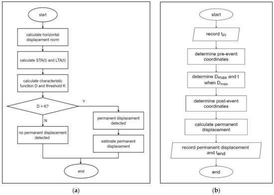
Figure 3.
Flowchart of the algorithm: (a) permanent displacement detection; (b) permanent displacement estimation.
3. Results
Two experimental stages were involved in this study, namely, tuning of the GA hyperparameters in the Okada–GA inversion model and testing of the model using the observation data. The scenarios and settings of each stage along with its results are outlined below.
3.1. GA Hyperparameter Tuning Experiments for Okada–GA Inversion Model
The purpose of the first-stage experiments in this study was to test the ability of the GAs to carry out inversion of Okada’s model to estimate four earthquake source parameters (i.e., length, width, rake, and slip) and to obtain the hyperparameter setting that resulted in the best performance of the Okada–GA inversion model.
3.1.1. Experimental Scenarios and Settings
In simple terms, the task of the GA in the Okada–GA inversion model was to convert the earthquake displacement value into the estimated parameters (i.e., length, width, rake, and slip) based on Okada’s inversion model. In this stage of the experiment, the displacement value used for the inversion was obtained from the forward calculation of Okada’s model using a predetermined earthquake fault model. The displacement was referred to as Okada’s displacement. As Okada’s model involves observation points in its forward calculation, this stage of the experiment used 737 GPS stations related to the 2011 Tohoku Oki earthquake as the observation points. Hence, the fault model used in the experiment was also the fault model of the 2011 Tohoku Oki earthquake event. To obtain valid results for the GA performance when performing the inversion of Okada’s model, more than one fault model was used for the experiment. The four predetermined earthquake fault models used in this stage of the experiment are shown in Table 1.

Table 1.
Earthquake fault models used in the first stage of the experiment.
The first model was based on prior knowledge about the 2011 Tohoku Oki earthquake, the second model referred to a study published formally by the Tectonics Observatory California Institute of Technology [37], and the third and fourth models were based on models published by the Geospatial Information Authority of Japan (GSI) [38]. Figure 4 shows the fault model and distribution of observation points in the experiment.
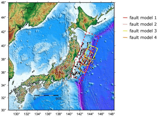
Figure 4.
Distribution of observation points, focal mechanism of the 2011 earthquake, and aftershocks.
To obtain a reliable estimation and represent the actual conditions of the data, some random error values were added to Okada’s displacement; these values were about 2–5 mm for each displacement value in the horizontal component. Both the forward and the inversion calculations of Okada’s model in this experiment involved the 737 GPS stations as observation points.
As noted earlier, all parameters of each fault model presented in Table 1 were used as input for the forward calculation of Okada’s model to generate Okada’s displacement. In this stage of experiment, the Okada’s displacement of each fault model was inversed using the GA to obtain four source parameters (i.e., the length, width, rake, and slip of the fault plane) by searching for the optimum solution that yielded the minimum fitness function. The range of search values for each estimated parameter and its data type were previously described in Section 2.2.1. From the estimated parameters obtained using the GA, the estimated displacement was calculated using Okada’s model. In this study, the estimated displacement was referred to as GA displacement.
GA performance strongly relies on the hyperparameter settings. Therefore, this study also included the tuning process in its experiments. In this stage, the hyperparameters of the GA were tuned to obtain the optimal estimation results. These hyperparameters included the number of generations (), size of the population (), number of chromosome bits (), crossover rate (), and mutation rate (). The previously mentioned tournament selection hyperparameter was set as a fixed parameter in the experiment: . Each hyperparameter combination generated in the tuning process was tested on the four fault models using the two objective functions described previously. At the end of the tuning process, the optimal set of hyperparameters along with the optimal objective function were selected for each fault model.
The values set for each hyperparameter tuned in the experiments are outlined in Table 2. According to the number of values of each hyperparameter, 108 hyperparameter combinations were generated for each combination of fault model and objective function. Hence, a total number of 864 experiments were run in the hyperparameter tuning process, with different hyperparameter settings for each. The Okada–GA inversion model was run for each experiment. All experiments in this study were run using Python programming on a computer with the following hardware specification: 16 GB RAM DDR4 and 4.2 GHz processor.
Table 2.
Hyperparameter values in the tuning process.
3.1.2. Hyperparameter Tuning Results
Based on the experimental results obtained from the hyperparameter tuning process, the GA performance in the Okada–GA inversion model was measured using the following parameters:
- (1).
- The displacement error value, which was defined as the difference between GA displacement and Okada’s displacement. This displacement error value was represented by using the RMSE of all the displacement values generated at each observation point. The error value was referred to as the parameter;
- (2).
- The estimated magnitude , which was generated by the GA estimation compared with the reference magnitude value generated from the calculation based on the length, width, and slip parameter values in the forward calculation of Okada’s model.
The best estimation result was the estimation with the minimal displacement error value and magnitude value error for all conducted experiments. Table 3 shows the best estimation result for each fault model tested in this stage of the experiment, compared with their original values as presented earlier in Table 1.
Table 3.
The best estimation results of the source parameters for each fault model tested.
Figure 5 compares GA displacement with Okada’s displacement for each fault model tested. Blue vectors represent GA displacement and black vectors represent Okada’s displacement. Coinciding vectors indicate that the estimation results are closer to the reference value. The red pentagram indicates the centroid of each fault model.
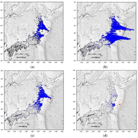
Figure 5.
Comparison of the displacements between the estimation (GA displacement) and the reference displacement (Okada’s displacement): (a) fault model 1; (b) fault model 2; (c) fault model 3; (d) fault model 4.
The hyperparameter combination settings shown in Table 3 that resulted in the best estimation performance were then selected to be used in the next stage of the experiment. The settings here included the number of generations, size of the population, number of chromosome bits, crossover rate, and mutation rate for each fault model. Table 4 shows the best configuration settings recommended by the tuning process for each fault model used.
Table 4.
The best configuration settings for each fault model.
In the following experiments, the selected objective function and hyperparameter setting shown in Table 4 were used to test the Okada–GA inversion model on real observation data, i.e., the GPS timeseries data from the 2011 Tohoku Oki and 2018 Lombok earthquake events.
3.2. Testing the Okada–GA Inversion Model Using the Observation Data
The testing in this step aimed to measure the ability of the Okada–GA inversion model to estimate source parameters from the real data of an earthquake. The estimated parameters were the same as those used in the previous stage (i.e., length, width, rake, and slip), in addition to the magnitude of the earthquake. In this stage, the GA with the best hyperparameter settings and the selected objective function was tested on the real displacement time series data from two earthquake events, i.e., the 2011 Tohoku Oki and 2018 Lombok earthquake events.
For all experiments carried out in this stage, the difference between the estimated parameters and reference parameters was expressed as the RMSE using the following standard formula:
where is the th estimated value, is the th reference value, and is the number of data points.
The results of the testing for each data event are described in the following sections.
3.2.1. The 2011 Tohoku Oki Earthquake Event
The time series data used for the testing were 1 Hz real-time kinematic-GPS data recorded at 737 observation points during this major earthquake. Here, the displacement of the 2011 Tohoku Oki earthquake was first calculated using the permanent displacement detection and estimation formula [5] described earlier. The displacement result from the formula using the real GPS time series data is referred to, in the next section, as the referenced permanent displacement. From the permanent displacement detection and calculation process, information about the permanent displacement detection and estimation time needed by each GPS station was obtained. Figure 6 shows the number of GPS stations involved in the calculation of the permanent displacement completed at a certain elapsed time . The estimated permanent displacement was then inversed using the GA to obtain the estimated source parameters.
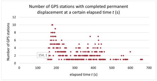
Figure 6.
Number of GPS stations with completed permanent displacement as input for the Okada–GA inversion at a certain elapsed time .
The permanent displacement results were used as input for the Okada–GA inversion model. The fault centroid, depth, strike, and dip parameters used for the inversion were the same parameters of the fault models used in the previous stage of the experiment. Comparison between the GA displacements and the referenced permanent displacement can be seen in Figure 7. The blue vectors are GA displacements, and the black vectors are the referenced permanent displacements of the 2011 Tohoku Oki earthquake event. The red pentagram indicates the centroid of each fault model.
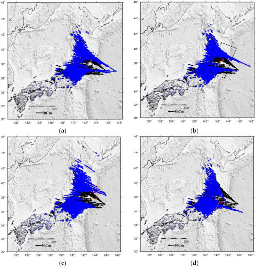
Figure 7.
Comparison of GA displacement and referenced permanent displacement of the 2011 Tohoku Oki earthquake: (a) fault model 1; (b) fault model 2; (c) fault model 3; (d) fault model 4.
The estimation results for the 2011 Tohoku Oki earthquake’s source parameters of each fault model are shown in Table 5. Table 5 also presents the between the GA displacement and referenced permanent displacement obtained from the permanent displacement formula [5] using the real time series data of 2011 Tohoku Oki earthquake event. The is illustrated earlier in Figure 7.
Table 5.
The estimation results of the 2011 Tohoku Oki earthquake’s source parameters using real observation data.
From the estimated results of the length, width, rake, and slip of the parameters, the value was estimated using Equations (7) and (8). Table 3 and Table 5 show the estimated results of for the first and second stages of the experiment, respectively.
In this stage of the experiment, in addition to the displacement results to be used as input into the GA, information about the elapsed time required by each GPS station was also retrieved to complete the permanent displacement formula as shown in Figure 6. Here, is the elapsed time required to complete the calculation of the estimated permanent displacement, and is the GA computational time required to obtain the parameter estimation results and Mw, calculated from the time of the permanent displacement is input into the GA. Hence, the total elapsed time required by the Okada–GA inversion model proposed in this study to complete the source parameters and magnitude estimation () was as follows:
Table 6 shows the GA computational time required () to obtain the estimated source parameters and the estimated of the 2011 Tohoku Oki earthquake for each fault model tested in the experiment using the previously mentioned hardware specification.
Table 6.
The GA computational time required () in the case of the 2011 Tohoku Oki earthquake, for each fault model tested.
According to the data shown in Figure 6, Equation (14), and the data presented in Table 6, the progress of the estimation could be observed per elapsed time, as shown in Figure 8. The figure presents an update of the estimated value per unit of elapsed time for each fault model employed in the testing, starting from the elapsed time = 173.81 to = 713.13 s. The first estimation is obtained at the elapsed time = 173.81 s, which yields an value of 9.067 using fault model 4.
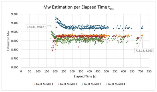
Figure 8.
Magnitude updates per unit of elapsed time (t) in the 2011 Tohoku Oki earthquake for each tested fault model calculated by the proposed method.
3.2.2. The 2018 Lombok Earthquake Event
The Okada–GA inversion model was also tested on the 2018 Lombok earthquake’s time series data. Due to limited observation data, the time series data used for testing were 1 Hz real-time kinematic-GPS data recorded at one observation point during this major earthquake. As in the testing experiment for the 2011 Tohoku Oki earthquake described previously, the displacement of the 2018 Lombok earthquake was first calculated. The displacement results were then used as input data for the Okada–GA inversion model.
In this testing experiment, the predetermined parameters used for the inversion, i.e., hypocenter location, strike, and dip, referred to the focal mechanism information published by the International Seismological Centre (ISC) [39], as can be seen in Table 7.
Table 7.
The predetermined source parameter of the 2018 Lombok earthquake event used for testing, and the referred .
The estimation results of the parameters length, width, rake, and slip were 73 km, 73 km, 60°, and 0.171 m, respectively. Figure 9 shows the comparison between the GA displacements and the referenced permanent displacement of the 2018 Lombok earthquake case. The GA displacement and the referenced displacement are represented by the blue vector and the black vector, respectively. The red pentagram indicates the epicenter of the 2018 Lombok earthquake.
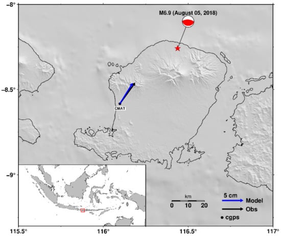
Figure 9.
Comparison of GA displacement and referenced permanent displacement of the 2018 Lombok earthquake.
From the source parameters estimation results, the estimation was calculated using Equations (7) and (8). The estimated result was 6.898, with the = 64 s and the = 28.263 s, using the hardware specification previously described. Hence, the total elapsed time required by the Okada–GA inversion model proposed in this study to complete the source parameters and magnitude estimation () of the 2018 Lombok earthquake event was 92.263 s.
4. Discussion
The estimation results of the first stage of the experiment in Table 3 showed that was, on average, 3.784 × 10⁻³ m for all the models or 3.572 × 10⁻³ m for the first model as the minimum error and 4.339 × 10⁻³ m for the maximum error value. These values indicated that the Okada–GA inversion model generated estimated displacements close to the referenced displacements. The estimation results for each parameter in each model were also close to the reference values in all fault models tested. This meant that the Okada–GA inversion model proposed in this study could provide relatively accurate estimation results. Figure 5 also showed that the GA displacements almost coincided with Okada’s displacements.
However, the estimation results in the second stage of the experiment were not as accurate as the first stage results. The average of in the second stage of the experiment (0.105 m) was larger than generated in the first experiment (3.78 × 10⁻³ m). In the first stage, the referenced displacement values were Okada’s displacements, which were fixed values generated from the forward calculation of Okada’s model. Meanwhile, in the second stage, the reference values were the real permanent displacement values estimated from the permanent displacement formula [5], which presented significant errors compared with Okada’s displacements.
According to the calculations using all the observation points, the average of in the RMSE between the real permanent displacements and Okada’s displacements was 0.083 m for the N components and 0.148 m for the E components. For the vertical components, the RMSE of in the Z components was 0.098 m.
The Okada–GA inversion model proposed in this study used Okada’s model as the main component of its objective function. Hence, the smaller the was between the real permanent displacement and Okada’s displacement, the smaller the RMSE was between GA displacement and the reference value, which was Okada’s displacement. Therefore, when the Okada–GA inversion model estimated the displacement values with real permanent displacement as its reference values, it was reasonable for the error difference to reach 0.105 m, but not when the Okada–GA inversion model estimated the displacement values using Okada’s displacements as its reference values.
However, the estimated result of each source parameter (length, width, rake, and slip) shown in Table 5 was reasonable according to the 2011 Tohoku Oki earthquake’s source model described and analyzed in previous research [40,41,42]. Some fault plane models analyzed in previous research ranged from 600 to 812 km in length and from 109 to 240 km in width [41,42], while the results estimated in this study used 668 km for the length parameter and 234 km for the width parameter in the third fault model tested. The range of estimated width parameter values that resulted from this study was between 153 to 234 km. The slip estimation value ranged between 25 and 60 m in most previous research [40,41], while this study estimated slips in the range of 10 to 24.598 km.
The estimation results in both the first and second stages of the experiment were also close to the reference values in each model, both in the 2011 Tohoku Oki and 2018 Lombok earthquake events. Furthermore, Figure 8 showed that the proposed method provided a relatively stable estimation value from early observations (elapsed time )—that is, as soon as a permanent displacement was detected and estimated. In the testing experiment on the 2011 Tohoku Oki earthquake’s data, the first estimations generated using each fault model in testing were 8.8, 8.823, 9.14, and 9.067 for fault model 1, 2, 3, and 4, respectively. In the 2018 Lombok earthquake testing, the estimation generated based on the single observation point was 6.898 which was close to the referenced , 6.9. Unlike the estimation results in previous studies, where the magnitude generally started with a low value [5,7,9,11,12,13], the first generated magnitude value that was estimated in this study was already close to the reference value and then increased or decreased slowly until it stabilized.
According to the data shown in Figure 6 and Figure 8, the first estimation generated in elapsed time was generated from the observation data of a single GPS station. The estimation value was relatively stable compared with the estimations at the following elapsed times generated from multiple GPS stations. In the case of the 2018 Lombok earthquake, due to the limited observation data, the estimation was also generated from a single GPS station. However, the estimation result was close to the referenced value of . It meant that in the proposed method, the number of GPS stations used as observation points did not significantly affect the values of the estimated parameter results.
The two main processes in the proposed model were permanent displacement estimation based on GPS time series data and the inversion of Okada’s model via GA to convert the displacement data into estimated source parameters. Hence, the proposed model has the potential to be applied to almost any earthquake case, as long as the earthquake causes surface deformation and significant permanent displacement that can be estimated using GPS time series data. However, the proposed model still requires some predetermined source parameters to perform the inversion, such as strike and dip parameters. Therefore, for different earthquake types such as an outer rise event, there may be constraints that need to be studied further in order for the model to estimate properly.
5. Conclusions
One crucial parameter must be estimated carefully when an earthquake occurs: the earthquake’s magnitude. Underestimating an earthquake’s magnitude will result in an inaccurate early warning and emergency response. This paper proposed a method using a GA to estimate four source parameters (i.e., length, width, rake, and slip). The proposed method can also estimate the moment magnitude with greater reliability and accuracy than previous methods, at least for the earthquake case analyzed in this study: the 2011 Japan Tohoku Oki earthquake. However, this method currently only estimates four source parameters and needs prior information to carry out the inversion. Hence, the model proposed in this study should be improved in future work.
Author Contributions
Conceptualization, A.N. and I.M.; methodology, A.N., I.M. and C.M.; software, A.N.; validation, C.M., S.W. and I.M.; formal analysis, A.N.; resources, A.N., I.M. and S.S.; writing—original draft preparation, A.N.; writing—review and editing, C.M., S.W., A.N. and I.M.; visualization, A.N. and S.S.; supervision, C.M., S.W. and I.M.; project administration, A.N. All authors have read and agreed to the published version of the manuscript.
Funding
This research was partially funded by the Institute of Technology Bandung (ITB) through the ITB competitive Research Program, grant number LPPM.PN-6-09-2021 and Indonesia Endowment Fund for Education (LPDP), grant number PRJ-102/LPDP/2021.
Conflicts of Interest
The authors declare no conflict of interest.
References
- Blewitt, G.; Hammond, W.C.; Kreemer, C.; Plag, H.P.; Stein, S.; Okal, E. GPS for Real-Time Earthquake Source Determination and Tsunami Warning Systems. J. Geod. 2009, 83, 335–343. [Google Scholar] [CrossRef]
- UNESCO; Indian Ocean Tsunami Warning and Mitigation System (IOTWS). Tsunami Warning and Mitigation Systems to Protect Coastal Communities; UNESCO: Paris, France, 2015. [Google Scholar]
- Agency for Meteorology Climatology and Geophysics Indonesia (BMKG). Indonesia Tsunami Early Warning System (InaTEWS) Concept and Implementation; German-Indonesian Cooperation for Tsunami Early Warning System (GITEWS): Jakarta, Indonesia, 2010.
- Branzanti, M.; Colosimo, G.; Crespi, M.; Mazzoni, A. GPS Near-Real-Time Coseismic Displacements for the Great Tohoku-Oki Earthquake. IEEE Geosci. Remote Sens. Lett. 2013, 10, 372–376. [Google Scholar] [CrossRef]
- Ohta, Y.; Kobayashi, T.; Tsushima, H.; Miura, S.; Hino, R.; Takasu, T.; Fujimoto, H.; Iinuma, T.; Tachibana, K.; Demachi, T.; et al. Quasi Real-Time Fault Model Estimation for near-Field Tsunami Forecasting Based on RTK-GPS Analysis: Application to the 2011 Tohoku-Oki Earthquake (M w 9.0). J. Geophys. Res. Solid Earth 2012, 117, B02311. [Google Scholar] [CrossRef]
- Plag, H.P.; Blewitt, G.; Bar-Sever, Y. Rapid Determination of Earthquake Magnitude and Displacement Field from GPS-Observed Coseismic Offsets for Tsunami Warning. In Proceedings of the 2012 IEEE International Geoscience and Remote Sensing Symposium, Munich, Germany, 22–27 July 2012; pp. 1182–1185. [Google Scholar] [CrossRef]
- Fang, R.; Shi, C.; Song, W.; Wang, G.; Liu, J. Determination of Earthquake Magnitude Using GPS Displacement Waveforms from Real-Time Precise Point Positioning. Geophys. J. Int. 2013, 196, 461–472. [Google Scholar] [CrossRef]
- Stramondo, S. The Tohoku-Oki Earthquake: A Summary of Scientific Outcomes from Remote Sensing. IEEE Geosci. Remote Sens. Lett. 2013, 10, 895–897. [Google Scholar] [CrossRef][Green Version]
- Wright, T.J.; Houlié, N.; Hildyard, M.; Iwabuchi, T. Real-Time, Reliable Magnitudes for Large Earthquakes from 1 Hz GPS Precise Point Positioning: The 2011 Tohoku-Oki (Japan) Earthquake. Geophys. Res. Lett. 2012, 39, 1–5. [Google Scholar] [CrossRef]
- Minson, S.E.; Simons, M.; Beck, J.L.; Ortega, F.; Jiang, J.; Owen, S.E.; Moore, A.W.; Inbal, A.; Sladen, A. Bayesian Inversion for Finite Fault Earthquake Source Models—II: The 2011 Great Tohoku-Oki, Japan Earthquake. Geophys. J. Int. 2014, 198, 922–940. [Google Scholar] [CrossRef]
- Muzli, M.; Asch, G.; Saul, J.; Murjaya, J. Rapid Moment Magnitude Estimation Using Strong Motion Derived Static Displacements. Procedia Earth Planet. Sci. 2015, 12, 11–19. [Google Scholar] [CrossRef]
- Melgar, D.; Crowell, B.W.; Geng, J.; Allen, R.M.; Bock, Y.; Riquelme, S.; Hill, E.M.; Protti, M.; Ganas, A. Earthquake Magnitude Calculation without Saturation from the Scaling of Peak Ground Displacement. Geophys. Res. Lett. 2015, 42, 5197–5205. [Google Scholar] [CrossRef]
- Leyton, F.; Ruiz, S.; Baez, J.C.; Meneses, G.; Madariaga, R. How Fast Can We Reliably Estimate the Magnitude of Subduction Earthquakes? Geophys. Res. Lett. 2018, 45, 9633–9641. [Google Scholar] [CrossRef]
- Cannavò, F. A New User-Friendly Tool for Rapid Modelling of Ground Deformation. Comput. Geosci. 2019, 128, 60–69. [Google Scholar] [CrossRef]
- Nagamani, A.N.; Anuktha, S.N.; Nanditha, N.; Agrawal, V.K. A Genetic Algorithm-Based Heuristic Method for Test Set Generation in Reversible Circuits. IEEE Trans. Comput. Des. Integr. Circuits Syst. 2018, 37, 324–336. [Google Scholar] [CrossRef]
- Gong, D.; Sun, J.; Miao, Z. A Set-Based Genetic Algorithm for Interval Many-Objective Optimization Problems. IEEE Trans. Evol. Comput. 2018, 22, 47–60. [Google Scholar] [CrossRef]
- Cunha, V.; Pessoa, L.; Vellasco, M.; Tanscheit, R.; Pacheco, M.A. A Biased Random-Key Genetic Algorithm for the Rescue Unit Allocation and Scheduling Problem. In Proceedings of the 2018 IEEE Congress on Evolutionary Computation, CEC 2018, Rio de Janeiro, Brazil, 8–13 July 2018; pp. 15–20. [Google Scholar] [CrossRef]
- Loohuis, J.; Van Eck, T. Simultaneous Focal Mechanism and Stress Tensor Inversion Using a Genetic Algorithm. Phys. Chem. Earth 1996, 21, 267–271. [Google Scholar] [CrossRef]
- Wu, Y.M.; Zhao, L.; Chang, C.H.; Hsu, Y.J. Focal-Mechanism Determination in Taiwan by Genetic Algorithm. Bull. Seismol. Soc. Am. 2008, 98, 651–661. [Google Scholar] [CrossRef]
- Velez, M.L.; Euillades, P.; Caselli, A.; Blanco, M.; Díaz, J.M. Deformation of Copahue Volcano: Inversion of InSAR Data Using a Genetic Algorithm. J. Volcanol. Geotherm. Res. 2011, 202, 117–126. [Google Scholar] [CrossRef]
- Asim, K.M.; Idris, A.; Iqbal, T.; Martínez-Álvarez, F. Seismic Indicators Based Earthquake Predictor System Using Genetic Programming and AdaBoost Classification. Soil Dyn. Earthq. Eng. 2018, 111, 1–7. [Google Scholar] [CrossRef]
- Mergos, P.E.; Sextos, A.G. Selection of Earthquake Ground Motions for Multiple Objectives Using Genetic Algorithms. Eng. Struct. 2019, 187, 414–427. [Google Scholar] [CrossRef]
- Růžek, B.; Kvasnička, M. Differential Evolution Algorithm in the Earthquake Hypocenter Location. Pure Appl. Geophys. 2001, 158, 667–693. [Google Scholar] [CrossRef]
- Zhou, Y.; Nie, Z.; Jia, Z. An Improved Differential Evolution Algorithm for Nonlinear Inversion of Earthquake Dislocation. Geod. Geodyn. 2014, 5, 49–56. [Google Scholar] [CrossRef][Green Version]
- Polyakov, Y.S.; Ryabinin, G.V.; Solovyeva, A.B.; Timashev, S.F. Is It Possible to Predict Strong Earthquakes? Pure Appl. Geophys. 2015, 172, 1945–1957. [Google Scholar] [CrossRef][Green Version]
- Wang, L.; Ding, R. Inversion and Precision Estimation of Earthquake Fault Parameters Based on Scaled Unscented Transformation and Hybrid PSO/Simplex Algorithm with GPS Measurement Data. Meas. J. Int. Meas. Confed. 2020, 153, 107422. [Google Scholar] [CrossRef]
- Wang, L.; Jin, X.; Xu, W.; Xu, G. A Black Hole Particle Swarm Optimization Method for the Source Parameters Inversion: Application to the 2015 Calbuco Eruption, Chile. J. Geodyn. 2021, 146, 101849. [Google Scholar] [CrossRef]
- Falcone, R.; Lima, C.; Martinelli, E. Soft Computing Techniques in Structural and Earthquake Engineering: A Literature Review. Eng. Struct. 2020, 207, 110269. [Google Scholar] [CrossRef]
- Stein, S.; Wysession, M. Focal Mechanism. In An Introduction to Seismology, Earthquakes, and Earth Structure; Blackwell Publishing: Hoboken, NJ, USA, 2003; p. 217. [Google Scholar]
- Segall, P. Earthquake and Volcano Deformation, 1st ed.; Princeton University Press: Princeton, NJ, USA, 2007. [Google Scholar]
- Okada, Y. Internal Deformation Due to Shear and Tensile Faults in a Half-Space. Bull. Seismol. Soc. Am. 1992, 82, 1018–1040. [Google Scholar] [CrossRef]
- The Clawpack Development Team. Earthquake Sources: Fault Slip and the Okada Model. Available online: https://www.clawpack.org/v5.5.x/okada.html (accessed on 16 December 2020).
- Zhang, Q.; Fang, W.; Sun, J.; Wang, Q. Improved Genetic Algorithm for High-Utility Itemset Mining. IEEE Access 2019, 7, 176799–176813. [Google Scholar] [CrossRef]
- Ye, M.; Wang, H. A Robust Adaptive Chattering-Free Sliding Mode Control Strategy for Automotive Electronic Throttle System via Genetic Algorithm. IEEE Access 2020, 8, 68–80. [Google Scholar] [CrossRef]
- Kochenderfer, M.J.; Wheeler, T.A. Algorithms for Optimization; MIT Press: London, UK, 2019. [Google Scholar]
- Hanks, T.C.; Kanamori, H. A Moment Magnitude Scale. J. Geophys. Res. B Solid Earth 1979, 84, 2348–2350. [Google Scholar] [CrossRef]
- Wei, S.; Sladen, A.; Group, A. Updated Result 3/11/2011 (Mw 9.0) Tohoku-Oki, Japan. Available online: http://www.tectonics.caltech.edu/slip_history/2011_tohoku-oki-tele/index.html (accessed on 4 February 2020).
- The Geospatial Information Authority of Japan. The 2011 Off the Pacific Coast of Tohoku Earthquake: Crustal Deformation and Fault Model. Available online: https://www.gsi.go.jp/cais/topic110422-index-e.html (accessed on 4 February 2020).
- ISC; TISC. ISC Bulletin: Focal Mechanism Search. Available online: http://www.isc.ac.uk/iscbulletin/search/fmechanisms/ (accessed on 10 June 2020).
- Zhou, X.; Cambiotti, G.; Sun, W.; Sabadini, R. The Coseismic Slip Distribution of a Shallow Subduction Fault Constrained by Prior Information: The Example of 2011. Geophys. J. Int. 2014, 199, 981–995. [Google Scholar] [CrossRef]
- Wang, Z.; Kato, T.; Zhou, X.; Fukuda, J. Source Process with Heterogeneous Rupture Velocity for the 2011 Tohoku-Oki Earthquake Based on 1-Hz GPS Data. Earth Planets Sp. 2016, 68, 193. [Google Scholar] [CrossRef]
- Uchida, N.; Burgmann, R. A Decade of Lessons Learned from the 2011 Tohoku-Oki Earthquake. Rev. Geophys. 2021, 59, 1–44. [Google Scholar] [CrossRef]


Publisher’s Note: MDPI stays neutral with regard to jurisdictional claims in published maps and institutional affiliations. |
© 2021 by the authors. Licensee MDPI, Basel, Switzerland. This article is an open access article distributed under the terms and conditions of the Creative Commons Attribution (CC BY) license (https://creativecommons.org/licenses/by/4.0/).