Interaction between Screw Dislocation and Interfacial Crack in Fine-Grained Piezoelectric Coatings under Steady-State Thermal Loading

Abstract

The mechanical behavior of fine-grained piezoelectric/substrate structure with screw dislocation and interface edge crack under the coupling action of heat, force and electricity are studied. Using the mapping function method, firstly, the finite area plane is transformed into the right semi-infinite plane, then the expression of the temperature field is given with the help of the complex function, and then the temperature field of the problem is achieved. By constructing the general solution of the governing equation with temperature function, the analytical expression of the image force is derived. Finally, the effects of material parameters, temperature gradient, coating thickness and crack size on image force are analyzed by numerical examples. The results show that the temperature gradient has a very significant effect on the image force, and thicker coating is conducive to the stability of dislocation and interface crack.

1. Introduction

Piezoelectric materials have been extensively used in aviation, aerospace, high-tech precision instruments, intelligent structures, structural health monitoring and other fields due to their unique properties. However, subject to the level of the manufacturing process and the piezoelectric composite structure in the process of serving local damage accumulation or format sample by work environment of the influence of the static, dynamic and random load also can produce all kinds of injury, when these defects and damage further expansion will lead to the overall structural failure, even resulting in economic losses and casualties. Therefore, it was particularly important to study the mechanical behavior of cracks and defects at the interface of piezoelectric composites, which attract a lot of attention [1,2,3,4,5,6]. Gao et al. [7,8] systematically studied the plane problem of piezoelectric material interface defects by using complex function method and Stroh theory. They obtained the piezoelectric materials containing an elliptic hole series approximate solution in the form of plane problems, and based on this as the basic solution of the boundary element method was used to solve more complex problems, at the same time as a special case degenerate elliptic holes crack were derived when the crack in the transverse isotropic piezoelectric body under the action of arbitrary concentrated force and concentrated charge of complex function. Xiao et al. [9] examined the interaction of screw dislocation, circular crack and inclusion in infinite single piezoelectric material under uniform heat flow, but did not discuss the case of piezoelectric composite material with finite size. Ueda [10] discussed the fracture of functionally gradient piezoelectric composites under multi-field coupling by using the Fourier integral transformation method. They calculated that increasing the material gradient helped to reduce the stress intensity factor under pure mechanical loads, and the crack length and material heterogeneity had a great effect on the temperature stress distribution but had a small effect on the electric displacement intensity factor under pure electric and thermal loads. Liu et al. [11,12] analytically the problems of screw dislocation and defects in one-dimensional hexagonal quasicrystal piezoelectric materials. They obtained the expressions of the stress field of screw dislocation and interface crack by using complex function method, and revealed the interaction between screw dislocation and stress field and the electric field by numerical examples. Lee and Pak [13] used the complex variable function and conformal transformation method was given in linear piezoelectric materials semi-infinite long crack and screw dislocation interaction explicit solution of the problem, after analysis found that the crack tip stress, electric displacement and electric field had a singularity, also discussed under the condition of the limit of power lost, the results were consistent with pure elastic situation. Gherrous et al. [14] derived the Griffith crack propagation problem at the interface of dual piezoelectric materials in semi-infinite planar structures. The solution of piezoelectric equation was transformed into singular integral equations by Fourier integral transformation, and the expression of the intensity factor. The numerical results demonstrate that the positive charge can prevent the crack propagation, and the material with smaller thickness and stronger rigidity can be selected to better resist the fracture. Nourazar et al. [15,16] investigated the fracture analysis of non-ideal piezoelectric coatings and orthotropic strips with multiple defects. Used the dislocation method, the problem was reduced to a singular integral equation and the effects of the non-ideal bonding coefficient, the defect geometry and coating properties on the stress intensity factor and the annular stress of the cavity were discussed numerically. Viun et al. [17] examined the plane strain problem of finite permeable piezoelectric bi-material interface cracks under load. They used complex function theory to transform the problem into a linear one, and given analytic expressions of the interface stress and crack tip strength factor in simple forms. Finally, by means of finite element method, the results of the influence of different polarization angles and different material combinations on fracture parameters were given. Shen et al. [18] explored the interaction between helical displacements and three different transverse isotropic piezoelectric semi-planar ternary composites and with hypotenuse cracks under mechanical loads in far-antiplane and in-plane electrical loads. The effects of crack length, crack angle and load position on electric field, stress field, generalized stress intensity factor, image force and crack propagation force were studied by the graphic method. Mishra et al. [19] dealed the interaction between multiple holes and cracks in piezoelectric devices under thermal-electro-mechanical loading environment. They used extended finite element method, interaction integral method and generalized Stroh formula to predict the stress intensity factor.

However, with the higher and higher requirements for precision instruments, ordinary piezoelectric materials can no longer meet the production requirements of high-end instruments, resulting in a series of new materials such as fine grain piezoelectric materials (the grain size is 100nm-10μm), nano piezoelectric materials. Reducing the particle size to the submicron level can improve the machinability of the material and the mechanical strength of the resulting device. In recent years, fine-grained piezoelectric materials have been used for cutting and grinding, and some high frequency transducers, microbrakes, and thin buzzers have been fabricated in which the advantages of fine-grained piezoelectric materials have been proved [20,21]. At the same time, many scholars have studied the relationship between grain size and mechanical properties and piezoelectric effect of dielectric piezoelectric materials through experiments [22,23,24]. However, the mechanical, dielectric and piezoelectric properties of fine-grained piezoelectric materials are uncertain with the grain size and preparation conditions, so the theoretical research on the defects of fine-grained piezoelectric materials mostly stays on the normal grain size, and the theoretical research on the interface defects of fine-grained piezoelectric materials was less.

In this paper, the interaction between screw dislocations and interface edge cracks in fine-grained piezoelectric/substrate structures under steady thermal loading was studied. By using the mapping function method, the problem of composite structure with finite thickness was transformed to the right half infinite plane structure. At the same time, the expression of the temperature field was given by using complex function method and Riemann–Schwartz analytic continuation theorem, and the temperature field was obtained. By using the theory of solution of linear equations, the solution of the governing equation with temperature function was regarded as the sum of one particular solution and the general solution of the corresponding governing equation in homogeneous form. According to the construction process of temperature field and the theoretical method adopted, the solution of the governing equation containing temperature function was constructed, and the theoretical expression of the image force was derived from it. Furthermore, the influence of various material parameters on image force were analyzed by numerical calculation.

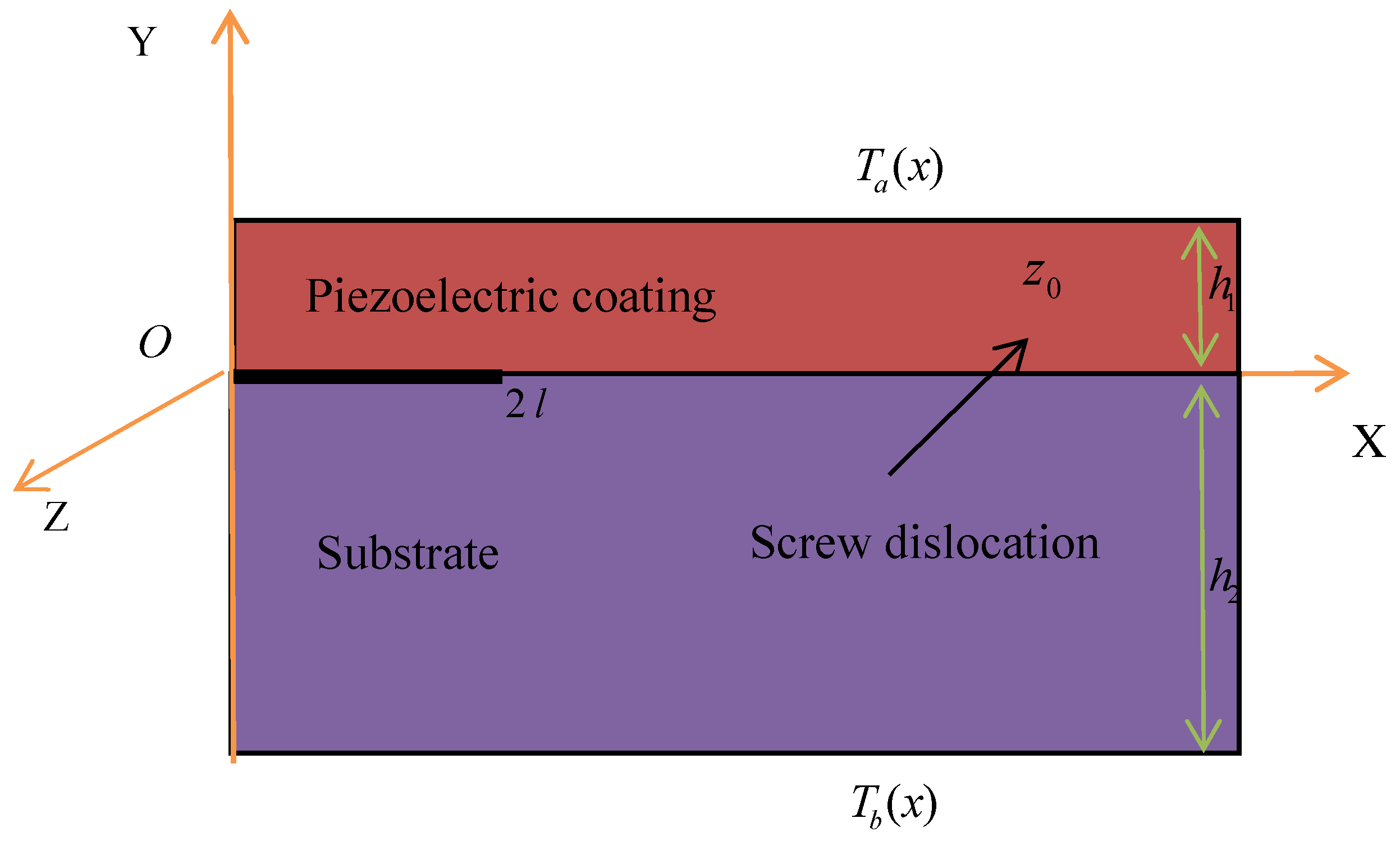
2. Problem Formulation

As shown in Figure 1, the fine-grained ceramic powder is prepared by high-efficiency mechanical ball milling, and then bonded with the substrate by plasma spraying technology to form the coating/substrate structure, while an open crack with a length of $2l$ is along the interface between the coating and substrate. A fine-grained piezoelectric coating/substrate structure was obtained by polarization treatment of coating. The coating is polarized along the $z$-axis. Assumed that coating and substrate are transversely isotropic. During the heating process of coating preparation, crystal deflection or bending may be caused, resulting in dislocation. Therefore, we assume that the screw dislocation $b=[b_z,b_{\varphi }]$ with dislocation line parallel to the poling direction are situated at $z_0$ in fine-grained piezoelectric coating, in which $b_z$ and $b_{\varphi }$ are the classical elastic displacement jump and the electric potential jump, respectively. The thickness of coating and substrate are $h_1$ and $h_2$, respectively. It is assumed that the crack faces remain thermally and electrically insulated and $T_a$, $T_b$ are environment temperature.

The control and constitutive equation of elastic field are [9]

$$\frac{\partial {\sigma }_{xz}}{\partial x}+\frac{\partial {\sigma }_{yz}}{\partial y}=0,\frac{\partial D_x}{\partial x}+\frac{\partial D_y}{\partial y}=0,$$

(1)

$${\sigma }_{xz}=c_{44}^{(n)}\frac{\partial W}{\partial x}+e_{15}^{(n)}\frac{\partial \Phi }{\partial x},$$

(2)

$${\sigma }_{yz}=c_{44}^{(n)}\frac{\partial W}{\partial y}+e_{15}^{(n)}\frac{\partial \Phi }{\partial y},$$

(3)

$$D_x=e_{15}^{(n)}\frac{\partial W}{\partial x}-{\epsilon }_{11}^{(n)}\frac{\partial \Phi }{\partial x}+p_1^{(n)}{T}_n,$$

(4)

$$D_y=e_{15}^{(n)}\frac{\partial W}{\partial y}-{\epsilon }_{11}^{(n)}\frac{\partial \Phi }{\partial y}+p_1^{(n)}{T}_n.$$

(5)

In Equations (1)–(5) the $W$, $\Phi$ are anti plane displacement and the electric potential, $c_{44}^{(n)}$ are elastic modulus, $e_{15}^{(n)}$ and ${\epsilon }_{11}^{(n)}$ are piezoelectric and dielectric constants, respectively. $T_n$ is the temperature change, ${\sigma }_{xz}$, ${\sigma }_{yz}$ are stress components, $D_x$ and $D_y$ are piezoelectric and dielectric constants, respectively. $p_1^{(n)}$ is pyroelectric constant. the superscript $n$ ($n=1,2$) stands for the fine-grained piezoelectric coating and piezoelectric substrate, respectively.

Assume that the temperature satisfies the Fourier heat conduction equation, as follows:

$$k_n^2\frac{{\partial }^2{T}_n}{\partial x^2}+\frac{{\partial }^2{T}_n}{\partial y^2}=0$$

(6)

where $k_n=\sqrt{\frac{k_x^{(n)}}{k_y^{(n)}}}$, $k_x^{(n)}$, $k_y^{(n)}$ are coefficients of thermal conductivity.

Substituting Equations (2)–(5) into Equation (1), we obtained

$$c_{44}^{(n)}{\nabla }^{2}W+e_{15}^{(n)}{\nabla }^2\Phi =0,$$

(7)

$$e_{15}^{(n)}{\nabla }^{2}W-{\epsilon }_{11}^{(n)}{\nabla }^2\Phi =-p_1^{(n)}(\frac{\partial T_n}{\partial x}+\frac{\partial T_n}{\partial y}), (n=1,2).$$

(8)

where ${\nabla }^2$ is the two-dimensional Laplacian operator.

For the homogeneous form of Equations (7) and (8), let

$$U={[W,\Phi ]}^T$$

The homogeneous form of Equations (7) and (8) can be rewritten as

$${\nabla }^{2}U=0.$$

(9)

Introduce the following variables

$$t_x={({\sigma }_{xz},D_x)}^T, t_y={({\sigma }_{yz},D_y)}^T.$$

(10)

The Equation (9) can be written as follows

$$t_x=L^{(n)}\frac{\partial U}{\partial x}, t_y=L^{(n)}\frac{\partial U}{\partial y}.$$

(11)

where

$$L^{(n)}=\left[\begin{array}{cc}{c}_{44}^{(n)}& e_{15}^{(n)}\\ e_{15}^{(n)}& -{\epsilon }_{11}^{(n)}\end{array}\right]$$

without loss of generality, the boundary conditions can be written as

$${\sigma }_{yz}(x,h_1)={\sigma }_{yz}(x,-h_2)=0, 0\le x<+\infty ,$$

(12)

$$D_y(x,h_1)=D_y(x,-h_2)=0, 0\le x<+\infty ,$$

(13)

$${\sigma }_{yz}(x,0^{+})={\sigma }_{yz}(x,0^{-}), \left|x\right|>a,$$

(14)

$$D_y(x,0^{+})=D_y(x,0^{-}), \left|x\right|>a,$$

(15)

$$W(x,0^{+})=W(x,0^{-}), \left|x\right|>a,$$

(16)

$$\Phi (x,0^{+})=\Phi (x,0^{-}), \left|x\right|>a,$$

(17)

$${\sigma }_{\mathrm{y}z}(x,0^{+})={\sigma }_{yz}(x,0^{-})=0, \left|x\right|\le a,$$

(18)

$$D_y(x,0^{+})=D_y(x,0^{-})=0, \left|x\right|\le a.$$

(19)

The thermal boundary conditions are specified as

$$T_n(x,0^{+})=T_n(x,0^{-}), \left|x\right|\ge a,$$

(20)

$$T_1(x,h_1)=T_a(x), T_2(x,h_2)=T_b(x), \left|x\right|\ge 0,$$

(21)

$$q_y^{(1)}(x,0)=q_y^{(2)}(x,0)=-q_0(x), \left|x\right|<a,$$

(22)

$$q_y^{(1)}(x,0)=q_y^{(2)}(x,0), \left|x\right|\ge a.$$

(23)

Considering that the temperature field does not depend on the stress field and displacement field, it can therefore, be calculated separately, and then the expressions of thermal stress and displacement field can be deduced in sequence.

3. Solution to the Problem

3.1. Temperature Field

According to reference [25], the finite interface region problem can be transformed into the right semi-infinite region problem by the following two mapping functions.

$$\zeta =-i{\left[\frac{1+i{e}^{\frac{\pi }{h_1+h_2}(z-\frac{h_1-h_2}{2})i}}{1-i{e}^{\frac{\pi }{h_1+h_2}(z-\frac{h_1-h_2}{2})i}}\right]}^2,$$

(24)

$$\xi =\sqrt{{\zeta }^2-a^2}.$$

(25)

From Equation (6), without losing generality, assuming that the thermal conductivity along X-axis and Y-axis is the same, that is, $k_x=k_y=k$, it can be obtained

$${\nabla }^{2}T=0$$

(26)

According to the theory of complex variable function, the solution of Equation (26) can be expressed in the following form

$$T=\mathrm{Im}{g}^{\prime }(\xi ).$$

(27)

where $g^{\prime }(\xi )$ is the temperature analytic function and $g(\xi )={[g_1(\xi ),g_2(\xi )]}^T$, $T={[T_1,T_2]}^T$, $\xi =x+iy$, Re and Im represent the real and imaginary parts of the complex potential function respectively.

Substitute Equation (27) into Equation (6), we obtain

$$q_x^{(n)}=-k_n\mathrm{Im}{g}^{\prime }(\xi ), q_y^{(n)}=-k_n\mathrm{Re}{g}^{\prime }(\xi ),$$

(28)

$$q_y^{(n)}+i{q}_x^{(n)}=-k_n{g}^{\prime }(\xi ).$$

(29)

where $q_x^{(n)}={[q_x^{(1)},q_x^{(2)}]}^T$, $q_y^{(n)}={[q_y^{(1)},q_y^{(2)}]}^T$.

According to reference [26], the function $g_2(\xi )$ in the $y\le 0$ plane can be written in the following form

$$g_2(\xi )=-\frac{h_0}{k_y^{(2)}}(1+i)\xi +o(\frac{1}{\xi }), \left|\xi \right|\to \infty .$$

(30)

At the same time, according to Riemann–Schwarz analytical continuation theorem, the function $g_2(\xi )$ in the whole plane has the following form

$$g_2(\xi )=\frac{h_0}{k_y^{(2)}}(1-i)\frac{1}{\xi }-\frac{h_0}{k_y^{(2)}}(1+i)\xi +g_{2*}(\xi ).$$

(31)

Similarly, let the function $g_1(\xi )$ have the following form in the $y\ge 0$ plane

$$g_1(\xi )=m\xi .$$

(32)

In the whole plane, the function $g_1(\xi )$ is extended to

$$g_1(\xi )=m\xi -\frac{\overline{m}}{\xi }+g_{1*}(\xi )$$

(33)

Here, $h_0$ represents the uniform heat flow components in the $\mathrm{X}$ and $\mathrm{Y}$ directions, $m$ is the undetermined complex number, and $g_{1*}(\xi )$ is a holomorphic function.

From the thermal boundary conditions (20), (23), we can obtain

$${[g_1(t)+g_2(t)]}^{+}={[g_1(t)+g_2(t)]}^{-},$$

(34)

$$k_y^{(1)}[g_1{(t)}^{+}+g_1{(t)}^{-}]=k_y^{(2)}[g_2{(t)}^{+}+g_2{(t)}^{-}]$$

(35)

According to Equations (30), (33) and (35), we obtain

$$g_1(\xi )+g_2(\xi )=[\frac{h_0(1-i)}{k_y^{(2)}}-\overline{m}]\frac{1}{\xi }+[m-\frac{h_0(1+i)}{k_y^{(2)}}]\xi .$$

(36)

According to Equations (34)–(36), we get

$$g_1{(t)}^{+}+g_1{(t)}^{-}=Q(t).$$

(37)

where

$$Q(t)=\frac{2k_y^{(2)}}{k_y^{(1)}+k_y^{(2)}}\{[\frac{h_0(1-i)}{k_y^{(2)}}-\overline{m}]\frac{1}{t}+[m-\frac{h_0(1+i)}{k_y^{(2)}}]t\}$$

According to Reference [27], the solution of Equation (37) can be expressed in the following form

$$g_1(\xi )=\frac{{\chi }_0(\xi )}{2\pi i}{\displaystyle \int \frac{Q(t)}{{\chi }_0(t)(t-\xi )}}dt.$$

(38)

where

$${\chi }_0(\xi )=\frac{1}{\sqrt{\xi (\xi -a)}}$$

By integrating Equation (38), we can get

$$g_1(z)=-\frac{{\chi }_0(z)}{2}[Q_0(z)+Q_{\infty }(z)]+\frac{Q(z)}{2}.$$

(39)

where

$$Q_0(\xi )=\frac{2k_y^{(2)}}{k_y^{(1)}+k_y^{(2)}}[\frac{h_0(1-i)}{k_y^{(2)}}-\overline{m}]\frac{1}{\xi },$$

(40)

$$Q_{\infty }(\xi )=\frac{2k_y^{(2)}}{k_y^{(1)}+k_y^{(2)}}\{[\frac{h_0(1-i)}{k_y^{(2)}}-\overline{m}]+[m-\frac{h_0(1+i)}{k_y^{(2)}}]\xi \sqrt{\xi (\xi -a)}\}.$$

(41)

Here, $Q_0(\xi )$ and $Q_{\infty }(\xi )$ are the singular principal parts of C at $z=0$ and $z=\infty$, respectively.

From Equations (36), (39)–(41), we obtained

$$g_1(\xi )=\frac{k_y^{(2)}}{k_y^{(1)}+k_y^{(2)}}[\frac{h_0(1-i)}{k_y^{(2)}}-\overline{m}]\frac{1}{\xi }-\frac{k_y^{(2)}}{k_y^{(1)}+k_y^{(2)}}\frac{1}{\sqrt{\xi (\xi -a)}}[\frac{h_0(1-i)}{k_y^{(2)}}-\overline{m}](\frac{1}{\xi }-1),$$

(42)

$$\begin{array}{l}{g}_2(\xi )=\frac{k_y^{(2)}}{k_y^{(1)}+k_y^{(2)}}\{[\frac{h_0(1-i)}{k_y^{(2)}}-\overline{m}]\frac{1}{\xi }+2[m-\frac{h_0(1+i)}{k_y^{(2)}}]\xi \}+\\ \frac{k_y^{(2)}}{k_y^{(1)}+k_y^{(2)}}\frac{1}{\sqrt{\xi (\xi -a)}}[\frac{h_0(1-i)}{k_y^{(2)}}-\overline{m}](\frac{1}{\xi }-1)\end{array}$$

(43)

when $\left|\xi \right|\to \infty$, it can be obtained from Equations (30) and (43)

$$m=0.$$

Further to collate Equations (40) and (41), we obtain

$$g_1(\xi )=\frac{k_y^{(2)}}{k_y^{(1)}+k_y^{(2)}}\frac{h_0(1-i)}{k_y^{(2)}}[\frac{1}{\xi }(1-\frac{1}{\sqrt{\xi (\xi -a)}})+\frac{1}{\sqrt{\xi (\xi -a)}}],$$

(44)

$$g_2(\xi )=\frac{k_y^{(2)}}{k_y^{(1)}+k_y^{(2)}}[\frac{h_0(1-i)}{k_y^{(2)}}(\frac{1}{\xi }+\frac{1}{\xi \sqrt{\xi (\xi -a)}}-\frac{1}{\sqrt{\xi (\xi -a)}})+\frac{2h_0(1+i)}{k_y^{(2)}}\xi ].$$

(45)

Substituting Equations (24) and (25) into Equations (44) and (45), we obtained

$$g_1(z)=\frac{k_y^{(2)}}{k_y^{(1)}+k_y^{(2)}}\frac{h_0(1-i)}{k_y^{(2)}}[\frac{1}{M_1}(1-\frac{1}{\sqrt{M_1(M_1-a)}})+\frac{1}{\sqrt{M_1(M_1-a)}}],$$

(46)

$$\begin{array}{l}{g}_2(z)=\frac{k_y^{(2)}}{k_y^{(1)}+k_y^{(2)}}[\frac{h_0(1-i)}{k_y^{(2)}}(\frac{1}{M_1}+\frac{1}{M_1\sqrt{M_1(M_1-a)}}-\frac{1}{\sqrt{M_1(M_1-a)}})\\ +\frac{2h_0(1+i)}{k_y^{(2)}}{M}_1]\end{array}$$

(47)

Substituting Equations (46) and (47) into Equation (27), the temperature field can be obtained as

$$\begin{array}{l}{T}_1=\frac{h_0(1-i)}{2(k_y^{(1)}+k_y^{(2)})}[\frac{1}{M_1}(1-\frac{1}{\sqrt{M_1(M_1-a)}})+\frac{1}{\sqrt{M_1(M_1-a)}}]-\\ \frac{h_0(1+i)}{(k_y^{(1)}+k_y^{(2)})}[\frac{1}{N_1}(1-\frac{1}{\sqrt{N_1(N_1-a)}})+\frac{1}{\sqrt{N_1(N_1-a)}}]\end{array}$$

(48)

$$\begin{array}{l}{T}_2=\frac{k_y^{(2)}}{2(k_y^{(1)}+k_y^{(2)})}[\frac{h_0(1-i)}{k_y^{(2)}}(\frac{1}{M_1}+\frac{1}{M_1\sqrt{M_1(M_1-a)}}-\frac{1}{\sqrt{M_1(M_1-a)}})\\ +\frac{2h_0(1+i)}{k_y^{(2)}}{M}_1]-\frac{k_y^{(2)}}{(k_y^{(1)}+k_y^{(2)})}[\frac{h_0(1+i)}{k_y^{(2)}}(\frac{1}{N_1}+\frac{1}{N_1\sqrt{N_1(N_1-a)}}-\frac{1}{\sqrt{N_1(N_1-a)}})\\ +\frac{2h_0(1-i)}{k_y^{(2)}}{N}_1]\end{array}$$

(49)

where

$$N_1=\sqrt{{\left[\frac{1+i{e}^{\frac{\pi }{h_1+h_2}(\stackrel{-}{z}-\frac{h_1-h_2}{2})i}}{1-i{e}^{\frac{\pi }{h_1+h_2}(\stackrel{-}{z}-\frac{h_1-h_2}{2})i}}\right]}^4-a^2}, M_1=\sqrt{{\left[\frac{1+i{e}^{\frac{\pi }{h_1+h_2}(z-\frac{h_1-h_2}{2})i}}{1-i{e}^{\frac{\pi }{h_1+h_2}(z-\frac{h_1-h_2}{2})i}}\right]}^4-a^2}.$$

3.2. Thermal Stress and Electric Displacement Field

According to the theory of solution of the equations, the solution of the in- homogeneous Equations (7) and (8) can be expressed as the sum of the general solution of the corresponding homogeneous equations and a particular solution of the in-homogeneous equation. Therefore, in the following discussion, we will construct the particular solution of Equations (7) and (8) and the corresponding general solution of homogeneous form.

Similar to the solution process of temperature field, the solution of homogeneous Equation (9) can be expressed as

$$U_p={[W_p,{\Phi }_p]}^T=\mathrm{Im}g(z).$$

(50)

Therefore, the stress and potential shift can be expressed as

$$t_x-i{t}_y=L^{(n)}G(z).$$

(51)

where

$$G(z)=g^{\prime }(z).$$

Substitute Equation (50) into Equations (7) and (8), we obtain

$${\nabla }^{2}W=-\frac{e_{15}^{(n)}p}{c_{44}^{(n)}{\epsilon }_{11}^{(n)}+e_{15}^{(n)}}[\mathrm{Im}{g}^{\prime }(z)-\mathrm{Re}{g}^{\prime }(z)],$$

(52)

$${\nabla }^2\Phi =\frac{c_{44}^{(n)}p}{c_{44}^{(n)}{\epsilon }_{11}^{(n)}+e_{15}^{(n)}}[\mathrm{Im}{g}^{\prime }(z)-\mathrm{Re}{g}^{\prime }(z)].$$

(53)

where $p={[p_1^{(1)},p_1^{(2)}]}^T$.

By solving the Equations (52) and (53), we can obtain

$$W=-\frac{e_{15}^{(n)}p}{8(c_{44}^{(n)}{\epsilon }_{11}^{(n)}+e_{15}^{(n)})}[(1+i)g(z)\overline{z}+(1-i)g(\overline{z})z]+g_w(z)+{\lambda }_w(\overline{z}),$$

(54)

$$\Phi =\frac{c_{44}^{(n)}p}{8(c_{44}^{(n)}{\epsilon }_{11}^{(n)}+e_{15}^{(n)})}[(1+i)g(z)\overline{z}+(1-i)g(\overline{z})z]+g_{\varphi }(z)+{\lambda }_{\varphi }(\overline{z}).$$

(55)

where $g_w(z)$, ${\lambda }_w(\stackrel{-}{z})$, $g_{\varphi }(z)$, ${\lambda }_{\varphi }(\stackrel{-}{z})$ are holomorphic functions.

According to the above discussion, the following functions may be taken as the special solutions of Equations (7) and (8)

$$U_q={[W_q,{\Phi }_q]}^T=\mathrm{Im}f(z).$$

(56)

where

$$f(z)=f_n(z)=\left[\begin{array}{c}-\frac{e_1^{(n)}{p}_1}{8(c_{44}^{(n)}{\epsilon }_{11}^{(n)}+e_{15}^{(n)})}[(1+i)g_n(z)\overline{z}+(1-i)g_n(\overline{z})z]+f_{n*}(z)\\ \frac{c_{44}^{(n)}{p}_1}{8(c_{44}^{(n)}{\epsilon }_{11}^{(n)}+e_{15}^{(n)})}[(1+i)g_n(z)\overline{z}+(1-i)g_n(\overline{z})z]+f_{n*}(z)\end{array}\right],$$

$$n=1,2.$$

(57)

Here, $f_{1*}(z)$ is a holomorphic function.

For the non-homogeneous Equations (7) and (8), the relationship between stress and potential shift is also obtained

$$t_x-i{t}_y=L^{(n)}{f}^{\prime }(z)+\left[\begin{array}{c}0\\ p_1^{(n)}\end{array}\right]T(1-i).$$

(58)

According to Equations (51), (57), the solutions of Equations (7) and (8) can finally be expressed as

$$U=\left[\begin{array}{c}W\\ \Phi \end{array}\right]=U_p+U_q=\mathrm{Im}[f(z)+g(z)].$$

(59)

Substituting Equation (46) into Equation (57) and find the derivative, then

$$f_1^{\prime }(z)=\left[\begin{array}{c}\begin{array}{l}-a_0{a}_2{a}_3[-\frac{1}{N_1}(1-\frac{1}{\sqrt{M_1(M_1-a)}})+(\frac{1}{M_1}-1)\frac{2M_1-a}{M_1(M_1-a)\sqrt{M_1(M_1-a)}})]+\\ [\frac{1}{\overline{z}}(1-\frac{1}{\sqrt{N_1(N_1-a)}})+\frac{1}{N_1}(1-\frac{1}{\sqrt{N_1(N_1-a)}})]+f_{1*}^{\prime }(z)\end{array}\\ \begin{array}{l}{a}_1{a}_2{a}_3[-\frac{1}{N_1}(1-\frac{1}{\sqrt{M_1(M_1-a)}})+(\frac{1}{M_1}-1)\frac{2M_1-a}{M_1(M_1-a)\sqrt{M_1(M_1-a)}})]+\\ [\frac{1}{N_1}(1-\frac{1}{\sqrt{N_1(N_1-a)}})+\frac{1}{N_1}(1-\frac{1}{\sqrt{N_1(N_1-a)}})]+f_{1*}^{\prime }(z)\end{array}\end{array}\right]$$

(60)

where

$$\begin{array}{c}{a}_0=\frac{e_{15}^{(1)}{p}_1}{8(c_{44}^{(1)}{\epsilon }_{11}^{(1)}+e_{15}^{(1)})}, a_2=\frac{k_y^{(2)}}{k_y^{(1)}+k_y^{(2)}}\frac{h_{0}i}{k_y^{(2)}}, \\ a_1=\frac{c_{44}^{(1)}{p}_1}{8(c_{44}^{(1)}{\epsilon }_{11}^{(1)}+e_{15}^{(1)})}, a_3=\frac{4\pi e^{\frac{\pi }{h_1+h_2}(z-\frac{h_1-h_2}{2})i}}{(h_1+h_2){(1-i{e}^{\frac{\pi }{h_1+h_2}(z-\frac{h_1-h_2}{2})i})}^2}.\end{array}$$

Similarly, let the function $f_2^{\prime }(z)$ have the following form

$$f_2^{\prime }(z)=-\frac{4h_0{a}_0}{k_y^{(2)}}(\overline{z}+\frac{1}{z^2\overline{z}}).$$

(61)

where

$$a_0=\left[\begin{array}{c}\frac{e_{15}^{(2)}{p}_1^{(2)}}{8(c_{44}^{(2)}{\epsilon }_{11}^{(2)}+e_{15}^{(2)})}\\ \frac{c_{44}^{(2)}{p}_1^{(2)}}{8(c_{44}^{(2)}{\epsilon }_{11}^{(2)}+e_{15}^{(2)})}\end{array}\right]$$

From Equations (60) and (61), we obtain

$$\begin{array}{l}{f}_1^{\prime }(z)+f_2^{\prime }(z)=\\ \left[\begin{array}{c}\begin{array}{l}-a_0{a}_2{a}_3[-\frac{1}{N_1}(1-\frac{1}{\sqrt{M_1(M_1-a)}})+(\frac{1}{M_1}-1)\frac{2M_1-a}{M_1(M_1-a)\sqrt{M_1(M_1-a)}})]\\ +[\frac{1}{\overline{z}}(1-\frac{1}{\sqrt{N_1(N_1-a)}})+\frac{1}{N_1}(1-\frac{1}{\sqrt{N_1(N_1-a)}})]+f_{1*}^{\prime }(z)\end{array}\\ \begin{array}{l}{a}_1{a}_2{a}_3[-\frac{1}{N_1}(1-\frac{1}{\sqrt{M_1(M_1-a)}})+(\frac{1}{M_1}-1)\frac{2M_1-a}{M_1(M_1-a)\sqrt{M_1(M_1-a)}})]\\ +[\frac{1}{N_1}(1-\frac{1}{\sqrt{N_1(N_1-a)}})+\frac{1}{N_1}(1-\frac{1}{\sqrt{N_1(N_1-a)}})]+f_{1*}^{\prime }(z)\end{array}\end{array}\right]\\ -\frac{4h_0{a}_0}{k_y^{(2)}}(\overline{z}+\frac{1}{z^2\overline{z}})\end{array}$$

(62)

Substituting Equation (62) into boundary continuity conditions (14)–(17), we can obtain

$$\begin{array}{l}{f}_1^{\prime }{(t)}^{+}+f_1^{\prime }{(t)}^{-}=\\ {(L^{(1)}+L^{(2)})}^{-1}{L}^{(2)}{a}_1{a}_2{a}_3\{[-\frac{1}{N_2}(1-\frac{1}{\sqrt{M_2(M_2-a)}})+(\frac{1}{M_2}-1)\\ \frac{2M_2-a}{M_2(M_2-a)\sqrt{M_2(M_2-a)}})]+\frac{1}{N_2\sqrt{N_2(N_2-a)}})\}-{(L^{(1)}+L^{(2)})}^{-1}{L}^{(2)}\\ \frac{4h_0{a}_0}{k_y^{(2)}}\frac{1}{M_2^2{N}_2}+{(L^{(1)}+L^{(2)})}^{-1}{p}_1^{(2)}\left[\begin{array}{c}0\\ 1\end{array}\right]\cdot [T_2(1-i)+\stackrel{}{\frac{1}{M_2^2}{T}_2}(1+i)]-{(L^{(1)}+L^{(2)})}^{-1}\\ p_1^{(1)}\left[\begin{array}{c}0\\ 1\end{array}\right][T_1(1-i)+\stackrel{}{\frac{1}{M_2^2}{T}_1}(1+i)]\end{array}$$

(63)

where

$$\begin{array}{c}{a}_1=\left[\begin{array}{c}\frac{e_{15}^{(1)}{p}_1}{8(c_{44}^{(1)}{\epsilon }_{11}^{(1)}+e_{15}^{(1)})}\\ \frac{c_{44}^{(1)}{p}_1}{8(c_{44}^{(1)}{\epsilon }_{11}^{(1)}+e_{15}^{(1)})}\end{array}\right],N_2=\sqrt{{\left[\frac{1+i{e}^{\frac{\pi }{h_1+h_2}(\overline{t}-\frac{h_1-h_2}{2})i}}{1-i{e}^{\frac{\pi }{h_1+h_2}(\overline{t}-\frac{h_1-h_2}{2})i}}\right]}^4-a^2},\\ M_2=\sqrt{{\left[\frac{1+i{e}^{\frac{\pi }{h_1+h_2}(t-\frac{h_1-h_2}{2})i}}{1-i{e}^{\frac{\pi }{h_1+h_2}(t-\frac{h_1-h_2}{2})i}}\right]}^4-a^2}.\end{array}$$

According to the solution method of Equation (37), we obtain

$$\begin{array}{l}{f}_1^{\prime }(z)={(L^{(1)}+L^{(2)})}^{-1}{L}^{(2)}{a}_1{a}_2{a}_3\{[-\frac{1}{N_1}(1-\frac{1}{\sqrt{M_1(M_1-a)}})+(\frac{1}{M_1}-1)\\ \frac{2M_1-a}{M_1(M_1-a)\sqrt{M_1(M_1-a)}})]+\frac{1}{N_1\sqrt{N_1(N_1-a)}})\}-{(L^{(1)}+L^{(2)})}^{-1}{L}^{(2)}\\ \frac{4h_0{a}_0}{k_y^{(2)}}\frac{1}{M_1^2{N}_1}+{(L^{(1)}+L^{(2)})}^{-1}{p}_1^{(2)}\left[\begin{array}{c}0\\ 1\end{array}\right]\cdot \{\frac{h_0}{k_y^{(2)}}(\frac{1}{M_1}-N_1)-(\frac{1}{M_1^2}-1)[\frac{1}{M_1}\\ (1-\frac{1}{\sqrt{M_1(M_1-a)}})+\frac{i}{N_1}(1-\frac{1}{\sqrt{N_1(N_1-a)}})]\}-{(L^{(1)}+L^{(2)})}^{-1}{p}_1^{(1)}\left[\begin{array}{c}0\\ 1\end{array}\right]\frac{h_0}{k_y^{(2)}}\\ (\frac{1}{M_1}+\frac{1}{N_1})\frac{1}{\sqrt{M_1(M_1-a)}}-{(L^{(1)}+L^{(2)})}^{-1}{L}^{(2)}[\frac{a_1{h}_0}{k_y^{(1)}+k_y^{(2)}}\frac{a{N}_1}{M_1}-\frac{4h_0{a}_0}{k_y^{(2)}}\frac{1}{M_1^2{N}_1}\\ +\frac{a_1{h}_0}{k_y^{(1)}+k_y^{(2)}}\frac{N_1}{M_1}]\frac{1}{\sqrt{M_1(M_1-a)}}\end{array}$$

(64)

$$\begin{array}{l}{f}_2^{\prime }(z)=a_1{a}_2{a}_3[-\frac{1}{N_1}(1-\frac{1}{\sqrt{M_1(M_1-a)}})+(\frac{1}{M_1}-1)\\ \frac{2M_1-a}{M_1(M_1-a)\sqrt{M_1(M_1-a)}})]+[\frac{1}{N_1}(1-\frac{1}{\sqrt{N_1(N_1-a)}})+\frac{1}{N_1}(1-\\ \frac{1}{\sqrt{N_1(N_1-a)}})]-\frac{4h_0{a}_0}{k_y^{(2)}}(N_1+\frac{1}{M_1^2{N}_1})-{(L^{(1)}+L^{(2)})}^{-1}{L}^{(2)}{a}_1{a}_2\{[-\frac{1}{N_1}(1-\\ \frac{1}{\sqrt{M_1(M_1-a)}})+(\frac{1}{M_1}-1)\frac{2M_1-a}{M_1(M_1-a)\sqrt{M_1(M_1-a)}})]+\frac{1}{N_1\sqrt{N_1(N_1-a)}})\}\\ -{(L^{(1)}+L^{(2)})}^{-1}{L}^{(2)}\frac{4h_0{a}_0}{k_y^{(2)}}\frac{1}{M_1^2{N}_1}+{(L^{(1)}+L^{(2)})}^{-1}{p}_1^{(2)}\left[\begin{array}{c}0\\ 1\end{array}\right]\{\frac{h_0}{k_y^{(2)}}(\frac{1}{M_1}-N_1)-(\frac{1}{M_1^2}\\ -1)[\frac{1}{M_1}(1-\frac{1}{\sqrt{M_1(M_1-a)}})+\frac{i}{N_1}(1-\frac{1}{\sqrt{N_1(N_1-a)}})]\}-{(L^{(1)}+L^{(2)})}^{-1}{p}_1^{(1)}\\ \left[\begin{array}{c}0\\ 1\end{array}\right]\frac{h_0}{k_y^{(2)}}(\frac{1}{M_1}+\frac{1}{N_1})\frac{1}{\sqrt{M_1(M_1-a)}}-{(L^{(1)}+L^{(2)})}^{-1}{L}^{(2)}[\frac{a_1{h}_0}{k_y^{(1)}+k_y^{(2)}}\frac{a{N}_1}{M_1}-\frac{4h_0{a}_0}{k_y^{(2)}}\\ \frac{1}{M_1^2{N}_1}+\frac{a_1{h}_0}{k_y^{(1)}+k_y^{(2)}}\frac{N_1}{M_1}]\frac{1}{\sqrt{M_1(M_1-a)}}\end{array}$$

(65)

Substituting Equations (57), (62) and (63) into Equations (2)–(5) can obtain the thermal stress and potential shift field of the problem.

3.3. Image Force

According to the above discussion, the general solution of Equations (6) and (7) can be written as:

$$U=\left[\begin{array}{c}W\\ \Phi \end{array}\right]=U_p+U_q=\mathrm{Im}[f(z)+g(z)].$$

(66)

Obviously, it satisfies the boundary continuity conditions (12)–(23).

According to Equations (51), (58) and (66), we obtain:

$$t_x-i{t}_y=L^{(n)}[g^{\prime }(z)+f^{\prime }(z)]+\left[\begin{array}{c}0\\ p_1^{(n)}\end{array}\right]T(1-i).$$

(67)

According to reference [2], the image force acting on the dislocation can be expressed as:

$$F_x-i{F}_y=i{b}^T[t_{xn}^0-i{t}_{yn}^0], n=1,2,$$

(68)

where

$$t_{xn}^0-i{t}_{yn}^0=\underset{z\to z_0}{\lim }(t_{xn}-i{t}_{yn}).$$

(69)

Substituting Equations (44), (48), (64) into Equations (67)–(69), the image force expression can be obtained:

$$\begin{array}{l}{F}_x-i{F}_y=i{b}^T\{L^{(1)}\{\{\frac{h_0(1-i)}{k_y^{(1)}+k_y^{(2)}}[-\frac{1}{M_0^2}(1-\frac{1}{\sqrt{M_0(M_0-a)}})\\ +(M_0-1)\frac{2M_0-a}{2M_0\sqrt{M_0(M_0-a)}}]\}+{(L^{(1)}+L^{(2)})}^{-1}{L}^{(2)}{a}_1{a}_2{a}_3\\ \{[-M_0(1-\frac{1}{\sqrt{M_0(M_0-a)}})+(\frac{1}{M_0}-1)\frac{2M_0-a}{M_0(M_0-a)\sqrt{M_0(M_0-a)}})]\\ +\frac{1}{M_0\sqrt{M_0(M_0-a)}})\}-{(L^{(1)}+L^{(2)})}^{-1}{L}^{(2)}\frac{4h_0{a}_0}{k_y^{(2)}}\frac{1}{M_0^3}+{(L^{(1)}+L^{(2)})}^{-1}\\ p_1^{(2)}\left[\begin{array}{c}0\\ 1\end{array}\right]\cdot \{\frac{h_0}{k_y^{(2)}}(\frac{1}{M_0}-M_0)-(\frac{1}{M_0^2}-1)[\frac{1}{M_0}(1-\frac{1}{\sqrt{M_0(M_0-a)}})+\frac{i}{M_0}\\ (1-\frac{1}{M_0(M_0-a)})]\}-{(L^{(1)}+L^{(2)})}^{-1}{p}_1^{(1)}\left[\begin{array}{c}0\\ 1\end{array}\right]\frac{2h_0}{k_y^{(2)}}\frac{1}{M_0\sqrt{M_0(M_0-a)}}-\\ {(L^{(1)}+L^{(2)})}^{-1}{L}^{(2)}[\frac{a_1{h}_{0}a}{k_y^{(1)}+k_y^{(2)}}-\frac{4h_0{a}_0}{k_y^{(2)}}\frac{1}{M_0^3}+\frac{a_1{h}_0}{k_y^{(1)}+k_y^{(2)}}]\frac{1}{\sqrt{M_0(M_0-a)}}]\}\\ +\left[\begin{array}{c}0\\ p_1^{(1)}\end{array}\right]\cdot \{\frac{-h_{0}i}{(k_y^{(1)}+k_y^{(2)})}[\frac{1}{M_0}(1-\frac{1}{\sqrt{M_0(M_0-a)}})+\frac{1}{\sqrt{M_0(M_0-a)}}]-\\ \frac{h_0(1+i)}{(k_y^{(1)}+k_y^{(2)})}[\frac{1}{M_0}(1-M_0(M_0-a))+\frac{1}{\sqrt{M_0(M_0-a)}}]\}\}\end{array}$$

(70)

where

$$M_0=\sqrt{{\left[\frac{1+i{e}^{\frac{\pi }{h_1+h_2}(z_0-\frac{h_1-h_2}{2})i}}{1-i{e}^{\frac{\pi }{h_1+h_2}(z_0-\frac{h_1-h_2}{2})i}}\right]}^4-a^2}$$

Take the real part and imaginary part of Equation (70) respectively to obtain the image force along the x-axis and y-axis.

4. Numerical Example

We select cadmium selenide piezoelectric ceramics as the base material and fine-grained cadmium selenide piezoelectric ceramics as the coating material. The material parameters are:

$$\begin{array}{c}{e}_{15}^{(2)}=-0.138 C/m^2, {\epsilon }_{11}^{(2)}=0.825\times {10}^{-10} C/Vm,\\ c_{44}^{(2)}=1.32\times {10}^{10} N/m^2, p_1^{(2)}=0.621\times {10}^6 N/m^{2}K.\end{array}$$

Assume $r_0/h_1=0.1$, $k_y^{(1)}=k_y^{(2)}$, $b=[b_z,0]$.

Substitute $z_0=r{e}^{i\theta }$ into Equation (60) to discuss the variation of image force with angle $\theta$.

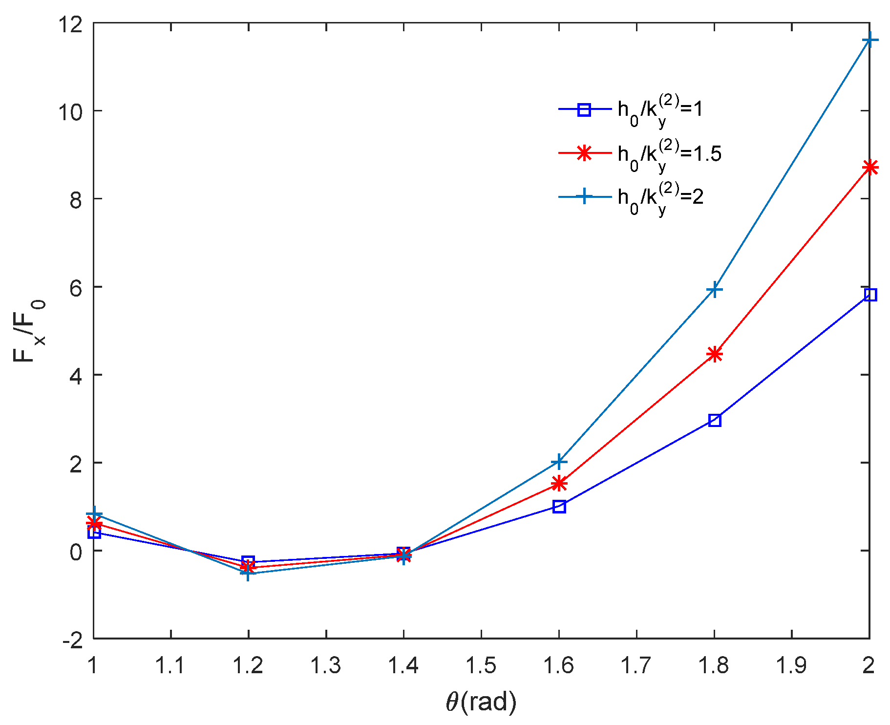
4.1. Effect of Temperature Gradient on Image Force

Figure 2 and Figure 3 show the variation law of image force with angle under different temperature gradients. The other parameters are: $h_2/h_1=100$, $h_1=1 \mathrm{mm}$, $c_{44}^{(1)}/c_{44}^{(2)}=1.5$, $a=1 \mathrm{mm}$, $F_0=c_{44}^{(2)}{b}_z^2/(h_1+h_2)$. The Figures shows that the image force $F_x$ first decreases and then increases with the increase of $\theta$, while the image force first increases and then decreases with the increase of $\theta$. At the same time, it is observed that the peak values of image force $F_x$ and $F_y$ change greatly for different temperature gradient values when $\theta \ge 1.4$, indicating that the influence of temperature gradient on image force is significant, but the image force changes little when $\theta \le 1.4$. On the other hand, it is found that the peak value of image force $F_x$ and $F_y$ increases with the increase of temperature gradient.

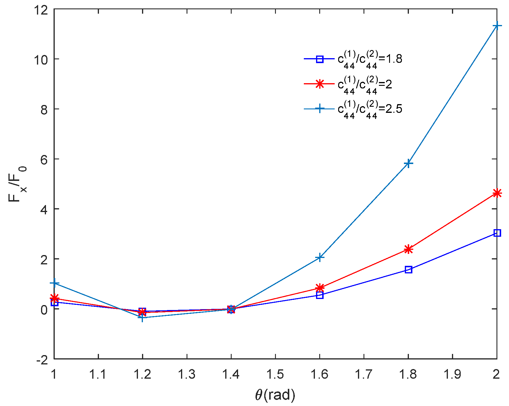
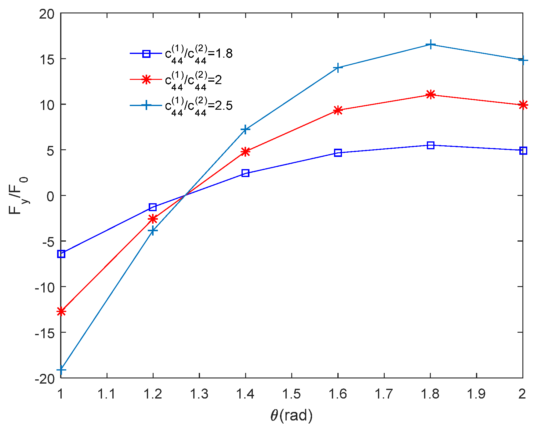
4.2. Effect of Material Elastic Modulus on Image Force

Figure 4 and Figure 5 shows the variation law of image force with angle under different elastic modulus ratio, and the other parameters are: $h_2/h_1=100$, $h_1=1\mathrm{mm}$, $h_0/k_y^{(2)}=1$, $a=1 \mathrm{mm}$, $F_0=c_{44}^{(2)}{b}_z^2/(h_1+h_2)$. It can be seen from the figures that the influence of elastic modulus on image force is similar to that of temperature gradient, that is, image force $F_x$ first decreases and then increases with the increase of $\theta$, while image force $F_y$ first increases and then decreases with the increase of $\theta$, however, the peak value of the image force corresponding to the elastic modulus is much larger than that corresponding to the temperature gradient, indicating that the influence of the elastic modulus of the material on the image force is more significant than that of the temperature gradient.

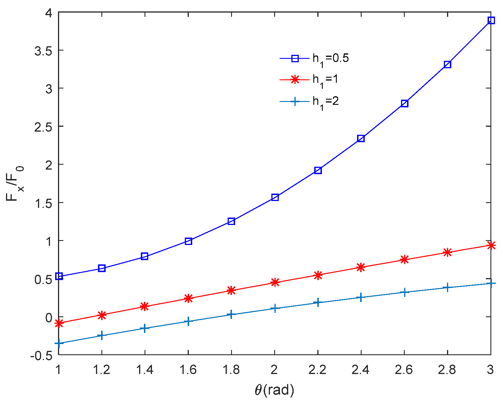
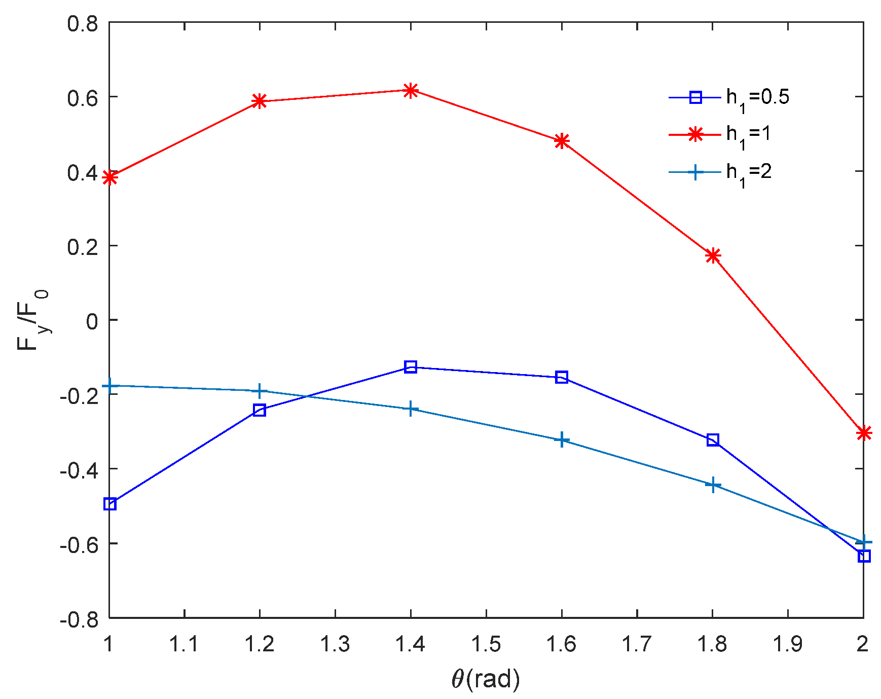
4.3. Effect of Coating Thickness on Image Force

Figure 6 and Figure 7 shows the variation law of image force with angle under different coating thickness, and the other parameters are: $h_2/h_1=100$, $c_{44}^{(1)}/c_{44}^{(2)}=1.5$, $h_0/k_y^{(2)}=1$, $a=1 \mathrm{mm}$, $F_0=c_{44}^{(2)}{b}_z^2/(h_1+h_2)$. It can be seen from the figures that image force $F_x$ increases with the increase of $\theta$, and image force $F_y$ first increases and then decreases with the increase of $\theta$, but for $h_1=2 \mathrm{mm}$, image force $F_y$ decreases with the increase of $\theta$. For the coating thickness $h_1$, when different values are taken, the image forces $F_x$ and $F_y$ show great changes, indicating that the coating thickness also has a great influence on the dislocation. It is also found that the peak value of image force decreases when the coating thickness is large.

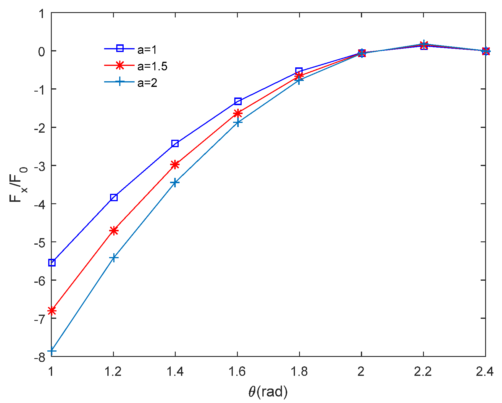
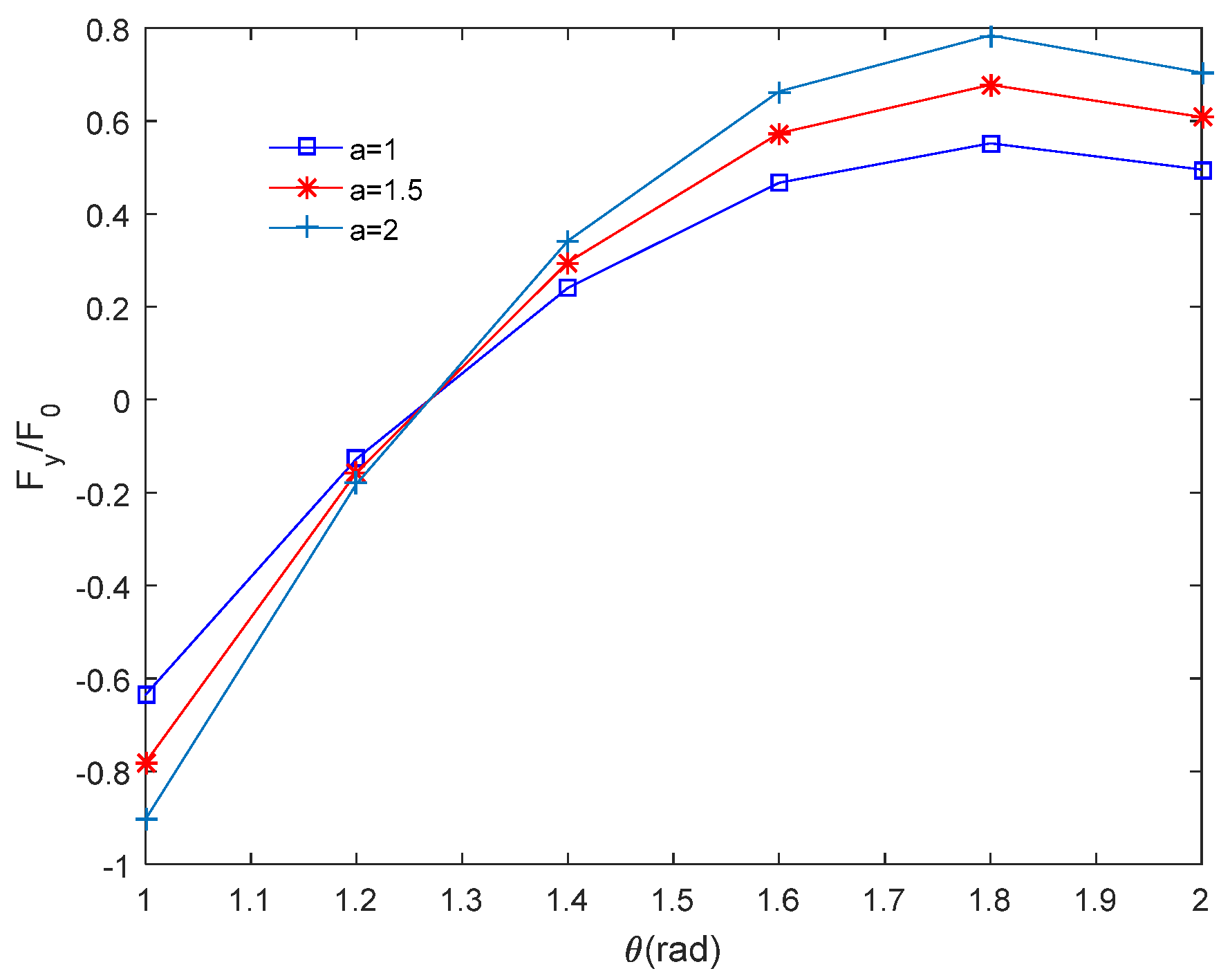
4.4. Effect of Crack Size on Image Force

Figure 8 and Figure 9 shows the variation law of image force with angle under the same crack length, and the other parameters are: $h_2/h_1=100$, $c_{44}^{(1)}/c_{44}^{(2)}=1.5$, $h_0/k_y^{(2)}=1$, $h_1=1 \mathrm{mm}$, $F_0=c_{44}^{(2)}{b}_z^2/(h_1+h_2)$. It can be seen from the figures that image force $F_x$ increases with the increase of $\theta$ and then tends to be stable, and image force $F_y$ first increases and then decreases with the increase of $\theta$. At the same time, when $\theta \ge 1.9$, the crack length has little effect on the image force $F_x$. Compared with other parameters, the effect of crack length on the image force is not so significant.

5. Discussion and Conclusions

In this paper, the interaction between screw dislocation and interfacial crack in fine-grained piezoelectric/substrate under steady-state thermal load is studied. The effects of material parameters, temperature gradient, coating thickness and crack size on image force are discussed through numerical examples. The results show that: (1) the image force increase with the increase of angle $\theta$, when $\theta \ge 1.4$ the growth rate of image force is obviously accelerated, and the temperature gradient has a very significant effect on the image force; (2) the peak value of image force corresponding to different elastic modulus ratio is larger than that corresponding to temperature gradient, indicating that influence of elastic modulus on image force is more significant than that of temperature gradient; (3) both coating thickness and crack size have an impact on the image force. The impact of crack size on the image force will gradually decrease with the increase of angle $\theta$. At the same time, the image force peak corresponding to a smaller coating thickness is less. Relatively speaking, a thicker coating helps to the stability of dislocations and interface cracks.

References

1. Pak, Y.E. Crack extension force in a piezoelectric material. Int. J. Appl. Mech. 1990, 57, 647–653. [Google Scholar] [CrossRef]
2. Pak, Y.E. Force on a Piezoelectric Screw Dislocation. Int. J. Appl. Mech. 1990, 57, 863–869. [Google Scholar] [CrossRef]
3. Suo, Z.; Kuo, C.M.; Barnett, D.M. Fracture mechanics for piezoelectric ceramics. J. Mech. Phys. Solids 1990, 40, 739–765. [Google Scholar] [CrossRef]
4. Park, S.; Sun, C.T. Fracture Criteria for Piezoelectric Ceramics. J. Am. Ceram. Soc. 1995, 78, 1475–1480. [Google Scholar] [CrossRef]
5. Liang, J.; Han, J.; Du, S. Rigid line inclusions and cracks in anisotropic piezoelectric solids. Mech. Res. Commun. 1995, 22, 43–49. [Google Scholar] [CrossRef]
6. Liu, J.X.; Lee, K.Y. Electroelastic behavior of arectangular piezoelectric ceramic with an anti-plane shear crack at arbitrary position. Eur. J. Mech. A-Solid. 2004, 23, 645–658. [Google Scholar] [CrossRef]
7. Gao, C.F.; Fan, W.X. An exact solution of crack problems in piezoelectric materials. Appl. Math. Mech.-Engl. 1999, 20, 51–58. [Google Scholar] [CrossRef]
8. Gao, C.F.; Fan, W.X. An interface inclusion between two dissimilar piezoelectric materials. Appl. Math. Mech.-Engl. 2001, 22, 96–104. [Google Scholar] [CrossRef]
9. Xiao, W.S.; Wei, G. The Interaction between Piezoelectric Screw Dislocation and Circular Crack under Remote Uniform Heat Flux. J. Hunan Univ. 2006, 33, 97–101. [Google Scholar] [CrossRef]
10. Ueda, S.; Okada, M.; Nakaue, Y. Transient thermal response of a functionally graded piezoelectric laminate with a crack normal to the bimaterial interface. J. Therm. Stresses 2017, 41, 98–118. [Google Scholar] [CrossRef]
11. Jiang, L.J.; Liu, G.T. The interaction between a screw dislocation and a wedge-shaped crack in one-dimensional hexagonal piezoelectric quasicrystals. Chin. Phys. B 2017, 26, 245–251. [Google Scholar] [CrossRef]
12. Lv, X.; Liu, G.T. Interaction between many parallel screw dislocations and a semi-infinite crack in a magnetoelectroelastic solid. Chin. Phys. B 2018, 27, 448–452. [Google Scholar] [CrossRef]
13. Lee, K.Y.; Lee, W.G.; Pak, Y.E. Interaction Between a Semi-Infinite Crack and a Screw Dislocation in a Piezoelectric Material. J. Appl. Mech. 2000, 67, 165–170. [Google Scholar] [CrossRef]
14. Gherrous, M.; Ferdjani, H. Analysis of a Griffith crack at the interface of two piezoelectric materials under anti-plane loading. Contin. Mech. Therm. 2016, 28, 1683–1704. [Google Scholar] [CrossRef]
15. Bayat, J.; Ayatollahi, M.; Bagheri, R. Fracture analysis of an orthotropic strip with imperfect piezoelectric coating containing multiple defects. Theor. Appl. Fract. Mech. 2015, 77, 41–49. [Google Scholar] [CrossRef]
16. Nourazar, M.; Ayatollahi, M. Analysis of an orthotropic strip containing multiple defects bonded between two piezoelectric layers. Acta Mech. 2016, 227, 1293–1306. [Google Scholar] [CrossRef]
17. Viun, O.; Komarov, A.; Lapusta, Y. A polling direction influence on fracture parameters of a limited permeable interface crack in a piezoelectric bi-material. Eng. Fract. Mech. 2018, 191, 143–152. [Google Scholar] [CrossRef]
18. Shen, M.H.; Hung, S.Y. Screw dislocation near a piezoelectric oblique edge crack. Meccanica 2016, 51, 1445–1456. [Google Scholar] [CrossRef]
19. Mishra, R.; Burela, R.G.; Pathak, H. Crack interaction study in piezoelectric materials under thermo-electro-mechanical loading environment. Int. J. Mech. Mater. Des. 2019, 15, 379–412. [Google Scholar] [CrossRef]
20. Xiao, C.J.; Li, Z.X.; Zhu, L.Y.; Zhang, H.T. Effect of grain size of BaTiO3 ceramics on thermal expansion and electrical properties. Int. J. Theor. Phys. 2014, 35, 346–351. [Google Scholar] [CrossRef]
21. Shi, Y.; Pu, Y.P.; Cui, Y.F.; Luo, Y.J. Enhanced grain size effect on electrical characteristics of fine grained BaTiO3 ceramics. J. Mater. Sci.-Mater. Electron. 2017, 28, 13229–13235. [Google Scholar] [CrossRef]
22. Martirena, H.T.; Burfoot, J.C. Grain-size effects on properties of some ferroelectric ceramics. J. Phys. C Solids Phys. 2001, 7, 3182–3192. [Google Scholar] [CrossRef] [Green Version]
23. Bell, A.J.; Moulson, A.J. The Effect of Grain Size on the Dielectric Properties of Barium Titanate Ceramic. J. Am. Ceram. Soc. 1985, 62, 325–328. [Google Scholar]
24. Lobo, R.P.S.M.; Mohallem, N.D.; Moreira, R.L. Grain size eff ect on diffuse phase transitions of sol-gel prepared barium titanate ceramics. J. Am. Ceram. Soc. 1995, 78, 1343–1346. [Google Scholar] [CrossRef]
25. Hu, S.S.; Liu, J.S.; Li, J.L.; Xie, X.F. Interaction of Screw Dislocation with Edge Interfacial Crack on Fine-Grained Piezoelectric Coating/Substrate. Adv. Mater. Sci. Eng. 2019, 2019, 1–13. [Google Scholar] [CrossRef] [Green Version]
26. Wang, X.; Shen, Y.P. A solution of the elliptical piezoelectric inclusion problem under uniform heat flux. Int. J. Solids Struct. 2001, 38, 2503–2516. [Google Scholar] [CrossRef]
27. Muskhelishvili, N.L. Some Basic Problems of the Mathematical Theory of Elasticity; Noordhoff International Publishing: Gromngen, The Netherlands, 1975. [Google Scholar] [CrossRef]
Figure 1. Mechanical model of fine-grained piezoelectric coating/substrate structure under steady-state thermal loading.
Applsci 11 11922 g001
Figure 2. Variation of image force F x with θ under different temperature gradients.
Applsci 11 11922 g002
Figure 3. Variation of image force F y with θ under different temperature gradients.
Applsci 11 11922 g003
Figure 4. Variation of F x / F 0 with θ under different elastic modulus ratios.
Applsci 11 11922 g004
Figure 5. Variation of F y / F 0 with θ under different elastic modulus ratios.
Applsci 11 11922 g005
Figure 6. Variation of F x / F 0 with θ under different coating thickness.
Applsci 11 11922 g006
Figure 7. Variation of F y / F 0 with θ under different coating thickness.
Applsci 11 11922 g007
Figure 8. Variation of F x / F 0 with θ under different crack lengths.
Applsci 11 11922 g008
Figure 9. Variation of F y / F 0 with θ under different crack lengths.
Applsci 11 11922 g009
Publisher’s Note: MDPI stays neutral with regard to jurisdictional claims in published maps and institutional affiliations.