
Overview of Tool Wear Monitoring Methods Based on Convolutional Neural Network


Abstract
:1. Introduction
2. Tool Wear Mechanism
3. Common Methods of Tool Wear Monitoring
4. Information Data of Indirect Online Measurement on Tool Wear
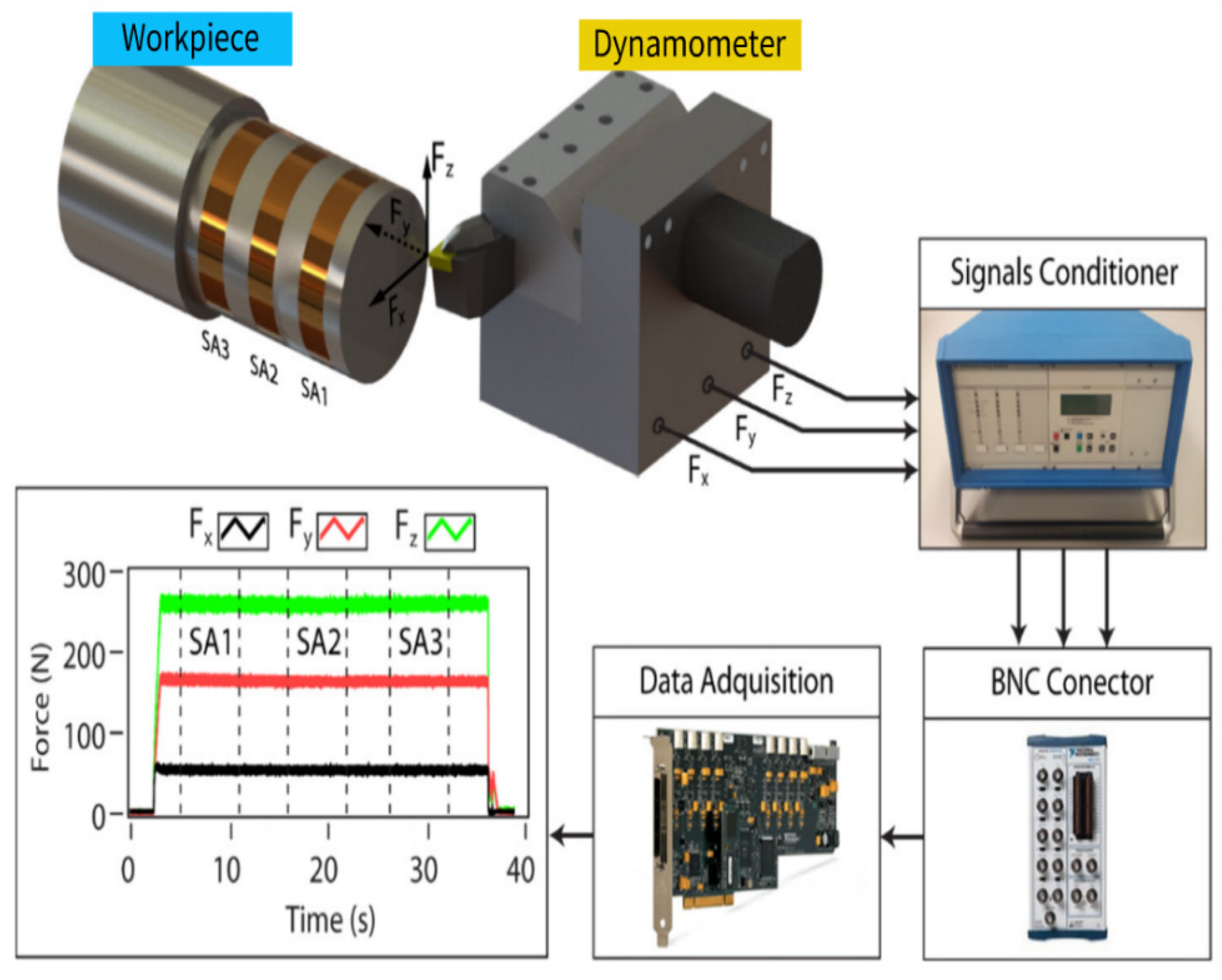
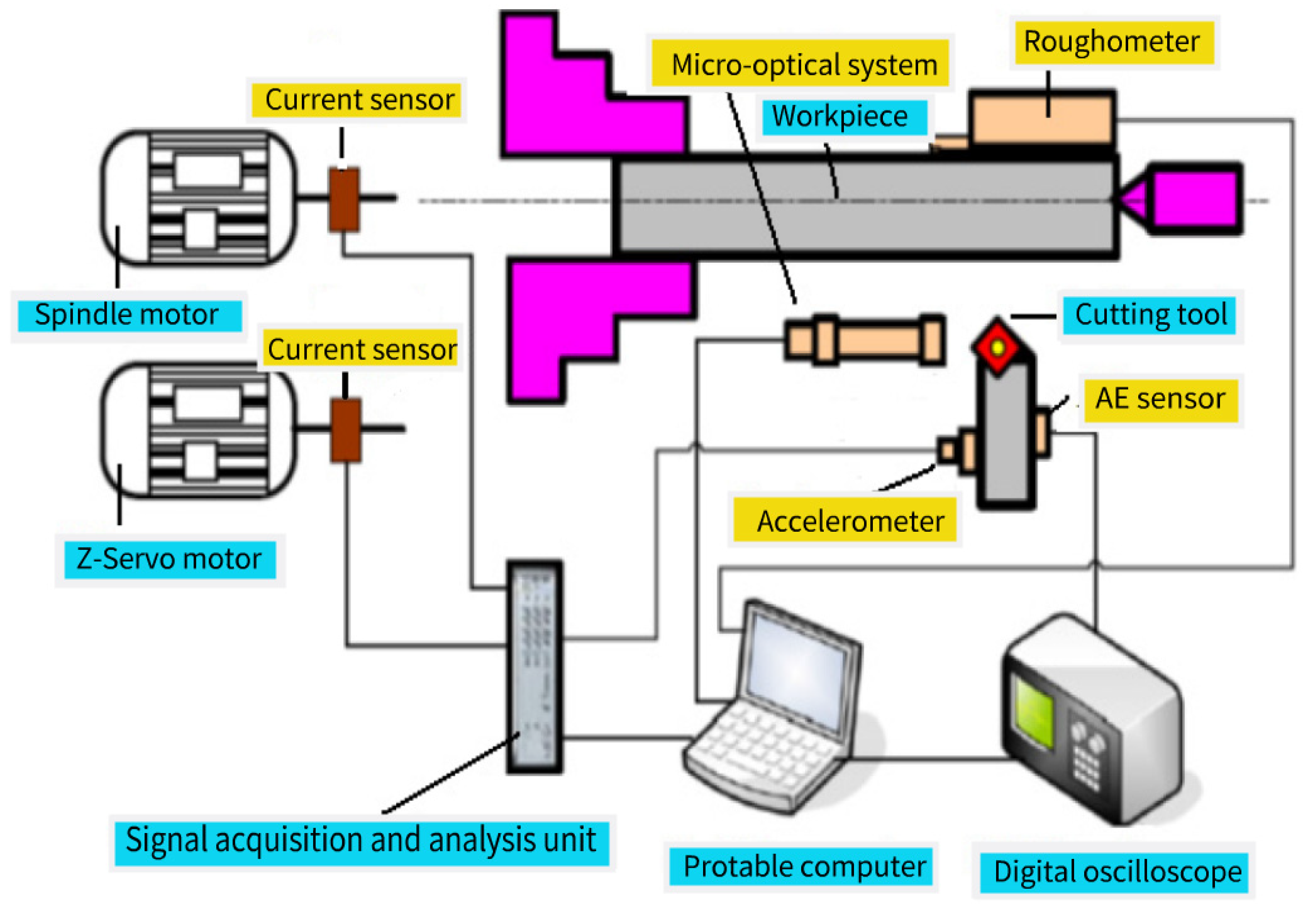
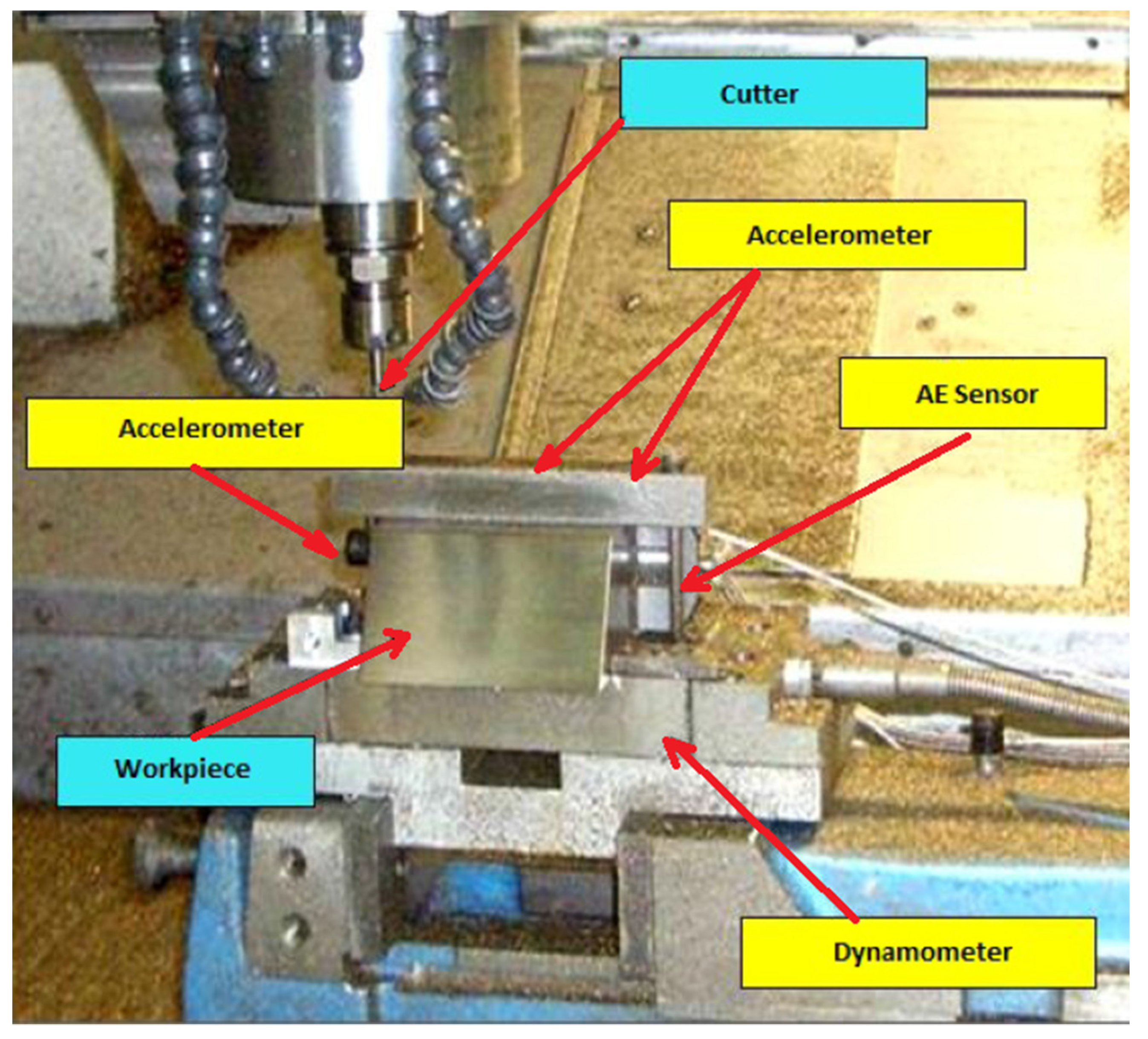
4.1. Cutting Force
4.2. Vibration
4.3. Acoustic Emission
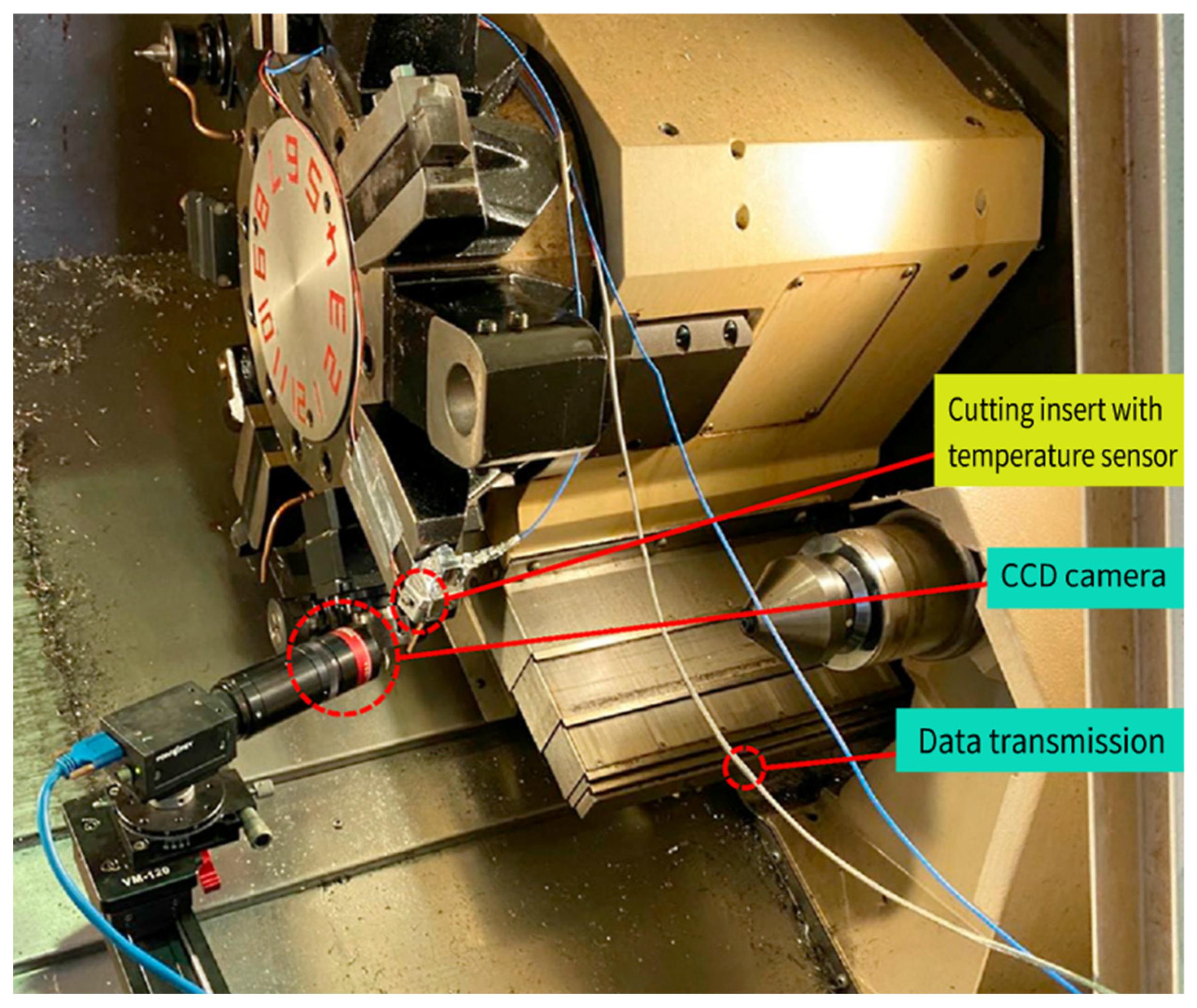
4.4. Temperature
4.5. Current
4.6. Power
4.7. Workpiece Surface Roughness
4.8. Multi-Information Fusion
5. Tool Wear Monitoring Method Based on Deep Convolutional Neural Network
5.1. Deep Convolutional Neural Network
5.2. Acquisition and Preprocessing of Tool Wear Monitoring Feature
5.3. Network Model Structure for Tool Wear Monitoring
5.4. Network Model Training
6. Existing Public Data Set
7. Challenges and Prospects
7.1. Challenges
7.2. Prospects
Author Contributions
Funding
Institutional Review Board Statement
Informed Consent Statement
Data Availability Statement
Conflicts of Interest
References
- Chen, J.; Hu, P.; Zhou, H.; Yang, J.; Xie, J.; Jiang, Y.; Gao, Z.; Zhang, C. Towards Intelligent Machine Tools. Engineering 2019, 5, 186–210. [Google Scholar] [CrossRef]
- Zhang, R. Overview of Intelligent Manufacturing Equipment Industry. Intell. Manuf. 2020, 7, 15–17. [Google Scholar]
- Ministry of Science and Technology of the People’s Republic of China. Special Plan for Scientific and Technological Innovation in the Field of Advanced Manufacturing Technology during the 13th Five-Year Plan Period (Selected). China Metrol. 2017, 12, 9–20. [Google Scholar]
- Siddhpura, A.; Paurobally, R. A review of flank wear prediction methods for tool condition monitoring in a turning process. Int. J. Adv. Manuf. Technol. 2013, 65, 371–393. [Google Scholar] [CrossRef]
- Fei, T.; He, Z.; Liu, A. Digital Twin in Industry: State-of-the-Art. IEEE Trans. Ind. Inform. 2019, 15, 2405–2415. [Google Scholar]
- Schleich, B.; Anwer, N.; Mathieu, L. Shaping the digital twin for design and production engineering. CIRP Ann.-Manuf. Technol. 2017, 66, 141–144. [Google Scholar] [CrossRef] [Green Version]
- Kritzinger, W.; Karner, M.; Traar, G. Digital Twin in manufacturing: A categorical literature review and classification. IFAC-Pap. 2018, 51, 1016–1022. [Google Scholar] [CrossRef]
- Bazaz, S.M.; Lohtander, M.; Varis, J. 5-Dimensional Definition for a Manufacturing Digital Twin. Procedia Manuf. 2019, 38, 1705–1712. [Google Scholar] [CrossRef]
- Botkina, D.; Hedlind, M.; Olsson, B.; Henser, J.; Lundholm, T. Digital Twin of a Cutting Tool. Procedia CIRP 2018, 72, 215–218. [Google Scholar] [CrossRef]
- Kejia, Z.; Zhenchuan, S.; Yaobing, S. Digital Twin-Driven Tool Wear Monitoring and Predicting Method for the Turning Process. Symmetry 2021, 13, 1438. [Google Scholar]
- Huibin, S.; Junlin, P.; Jiduo, Z.; Rong, M. Tool digital twin model for cutting process. Comput. Integr. Manuf. Syst. 2019, 25, 1474–1480. [Google Scholar]
- Congbo, L.; Xin, S.; Xiaobo, H.; Xikun, Z.; Shaoqing, W. On line monitoring method of NC milling tool wear driven by digital twin. China Mech. Eng. 2021, 1–11. Available online: http://kns.cnki.net/kcms/detail/42.1294.TH.20210519.1545.006.html (accessed on 13 December 2021).
- Lecun, Y.; Bengio, Y.; Hinton, G. Deep learning. Nature 2015, 521, 436–444. [Google Scholar] [CrossRef] [PubMed]
- Kalidass, S.; Palanisamy, P.; Muthukumaran, V. Prediction and optimization of tool wear for end milling operation using artificial neural networks and simulated annealing algorithm. Int. J. Mach. Mach. Mater. 2013, 14, 142–164. [Google Scholar]
- Chen, H.-Y.; Lee, C.-H. Deep Learning Approach for Vibration Signals Applications. Sensors 2021, 21, 3929. [Google Scholar] [CrossRef] [PubMed]
- Kuntoğlu, M.; Salur, E.; Gupta, M.K. A state-of-the-art review on sensors and signal processing systems in mechanical machining processes. Int. J. Adv. Manuf. Technol. 2021, 116, 2711–2735. [Google Scholar] [CrossRef]
- Kuntolu, M.; Aslan, A.; Pimenov, D.Y. A Review of Indirect Tool Condition Monitoring Systems and Decision-Making Methods in Turning: Critical Analysis and Trends. Sensors 2021, 21, 108. [Google Scholar] [CrossRef] [PubMed]
- Pimenov, D.Y.; Bustillo, A.; Mikolajczyk, T. Artificial intelligence for automatic prediction of required surface roughness by monitoring wear on face mill teeth. J. Intell. Manuf. 2017, 29, 1045–1061. [Google Scholar] [CrossRef] [Green Version]
- Zhiqiang, W.; Hu, G.; Fengzhou, F.; Bing, L. Application of length fractal dimension in identification of wear state of micro-milling cutter. Vibration. Test. Diagn. 2016, 36, 592–597. [Google Scholar]
- Kuntoglu, M.; Saglam, H. Investigation of signal behaviors for sensor fusion with tool condition monitoring system in turning. Measurement 2020, 173, 108582. [Google Scholar] [CrossRef]
- Rong, Z.; Weiping, L.; Tong, M. A review of research on deep learning. Inf. Control 2018, 47, 385–397. [Google Scholar]
- Jun, L.; Yongbao, L.; Youhong, Y. Application of convolutional neural network and kurtosis in bearing fault diagnosis. J. Aeronaut. Dyn. 2019, 34, 2423–2431. [Google Scholar]
- Zhou, Y.; Xue, W. Review of tool condition monitoring methods in milling processes. Int. J. Adv. Manuf. Technol. 2018, 96, 2509–2523. [Google Scholar] [CrossRef]
- Swain, S.; Panigrahi, I.; Sahoo, A.K. Adaptive tool condition monitoring system: A brief review. Mater. Today Proc. 2020, 23, 474–478. [Google Scholar] [CrossRef]
- Ms, A.; Mkg, B.; Itc, D. A state-of-the-art review on tool wear and surface integrity characteristics in machining of superalloys. CIRP J. Manuf. Sci. Technol. 2021, 35, 624–658. [Google Scholar]
- Kuntoğlu, M.; Sağlam, H. Investigation of Progressive Tool Wear for Determining of Optimized Machining Parameters in Turning. Measurement 2019, 7, 427–436. [Google Scholar] [CrossRef]
- Ghosh, N.; Ravi, Y.; Patra, A.; Mukhopadhyay, S.; Paul, S.; Mohanty, A.R.; Chattopadhyay, A.B. Estimation of tool wear during CNC milling using neural network-based sensor fusion. Mech. Syst. Signal Process 2007, 21, 466–479. [Google Scholar] [CrossRef]
- Cuka, B.; Kim, D.-W. Fuzzy logic based tool condition monitoring for end-milling. Robot. Comput.-Integr. Manuf. 2017, 47, 22–36. [Google Scholar] [CrossRef]
- Zel, T.; Karpat, Y. Predictive modeling of surface roughness and tool wear in hard turning using regression and neural networks. Int. J. Mach. Tools Manuf. 2005, 45, 467–479. [Google Scholar]
- Lee, S.; Chen, J. On-line surface roughness recognition system using artificial neural networks system in turning operations. Int. J. Adv. Manuf. Technol. 2003, 22, 498–509. [Google Scholar] [CrossRef]
- Wei, D.; Guofang, N. Application of CNN-RNN fusion method in fault diagnosis of rotating machinery. J. Light Ind. 2020, 35, 102–108. [Google Scholar]
- Zhiyuan, L.; Pengfei, M.; Jianglin, X.; Meiqing, W.; Xiaoqing, T. Online tool wear recognition method based on multi-source synchronized signals and deep learning. China Mech. Eng. 2019, 30, 220–225. [Google Scholar]
- Shuai, Z.; Yixiang, H.; Haoren, W.; Chengliang, L.; Xiao, L.; Xinguang, L. Tool wear assessment based on random forest and principal component analysis. Chin. J. Mech. Eng. 2017, 53, 181–189. [Google Scholar]
- Min, Y.; Mei, W.; Yuxia, P.; Maoqin, H. Feature selection method of milling force signal based on improved Drosophila optimization algorithm. Vib. Impact 2016, 35, 196–200. [Google Scholar]
- Bhuiyan, M.S.H.; Choudhury, I.A.; Dahari, M. Monitoring the tool wear, surface roughness and chip formation occurrences using multiple sensors in turning. J. Manuf. Syst. 2014, 33, 476–487. [Google Scholar] [CrossRef]
- Haijin, W.; Zongyu, Y.; Zhenzheng, K.; Yingjie, G.; Huiyue, D. Tool wear monitoring for spiral milling based on one-dimensional convolutional neural network. J. Zhejiang Univ. 2020, 54, 931–939. [Google Scholar]
- Dong, J.; Subrahmanyam, K.V.R.; Wong, Y.S.; Hong, G.S.; Mohanty, A.R. Bayesian-inference-based neural networks for tool wear estimation. Int. J. Adv. Manuf. Technol. 2006, 30, 797–807. [Google Scholar] [CrossRef]
- Nouri, M.; Fussell, B.K.; Ziniti, B.L. Real-time tool wear monitoring in milling using a cutting condition independent method. Int. J. Mach. Tools Manuf. 2015, 89, 1–13. [Google Scholar] [CrossRef]
- Dali, C.; Huibin, S.; Jiduo, Z.; Rong, M. Tool wear on-line monitoring based on convolutional neural network. Comput. Integr. Manuf. Syst. 2020, 26, 74–80. [Google Scholar]
- Javed, K.; Gouriveau, R.; Li, X. Tool wear monitoring and prognostics challenges: A comparison of connectionist methods toward an adaptive ensemble model. J. Intell. Manuf. 2018, 29, 1873–1890. [Google Scholar] [CrossRef]
- Lin, S.C.; Lin, R.J. Tool wear monitoring in face milling using force signals. Wear 1996, 198, 136–142. [Google Scholar] [CrossRef]
- Yan, W.; Wong, Y.S.; Lee, K.S. An investigation of indices based on milling force for tool wear in milling. J. Mater. Process. Technol. 1999, 89–90, 245–253. [Google Scholar] [CrossRef]
- Plaza, E.G.; Lopez, P.J.N. Analysis of cutting force signals by wavelet packet transform for surface roughness monitoring in CNC turning. Mech. Syst. Signal Process. 2018, 98, 634–651. [Google Scholar] [CrossRef]
- Altintas, Y.; Yellowley, I. In-Process Detection of Tool Failure in Milling Using Cutting Force Models. Trans. J. Eng. Ind 1989, 111, 149–157. [Google Scholar] [CrossRef]
- Kaya, B.; Oysu, C.; Ertunc, H. Force-torque based on-line tool wear estimation system for CNC milling of inconel 718 using neural networks. Adv. Eng. Softw. 2011, 42, 76–84. [Google Scholar] [CrossRef]
- Wang, M.; Wang, J. CHMM for tool condition monitoring and remaining useful life prediction. Int. J. Adv. Manuf. Technol. 2012, 59, 463–471. [Google Scholar] [CrossRef]
- Huang, P.; Ma, C.; Kuo, C. A PNN self-learning tool breakage detection system in end milling operations. Appl. Soft Comput. 2015, 37, 114–124. [Google Scholar] [CrossRef]
- Li, N.; Chen, Y.; Kong, D. Force-based tool condition monitoring for turning process using v-support vector regression. Int. J. Adv. Manuf. Technol. 2017, 91, 351–361. [Google Scholar] [CrossRef]
- Zhu, K.; Liu, T. On-line Tool Wear Monitoring via Hidden Semi-Markov Model with Dependent Durations. IEEE Trans. Ind. Inform. 2017, 99, 69–78. [Google Scholar]
- Jiaqi, H.; Yingguang, L.; Changqing, L. Real-time tool condition identification in milling based on cutting force signal-geometry information-process information. Aviat. Manuf. Technol. 2018, 61, 48–54. [Google Scholar]
- Prickett, P.; Johns, C. An overview of approaches to end milling tool monitoring. Int. J. Mach. Tools Manuf. 1999, 39, 105–122. [Google Scholar] [CrossRef]
- Koike, R.; Ohnishi, K.; Aoyama, T. A sensorless approach for tool fracture detection in milling by integrating multi-axial servo information. CIRP Ann.-Manuf. Technol. 2016, 65, 385–388. [Google Scholar] [CrossRef]
- Yesilyurt, I.; Ozturk, H. Tool condition monitoring in milling using vibration analysis. Int. J. Prod. Res. 2007, 45, 1013–1028. [Google Scholar] [CrossRef]
- Sevilla, P.; Robles, J.; Jauregui, J. FPGA-based reconfigurable system for tool condition monitoring in high-speed machining process. Measurement 2015, 64, 81–88. [Google Scholar] [CrossRef]
- Aslan, A. Optimization and Analysis of Process Parameters for Flank Wear, Cutting Forces and Vibration in Turning of AISI 5140: A Comprehensive Study. Measurement 2020, 163, 107959. [Google Scholar] [CrossRef]
- Ying, D.; Weixi, J.; Jiahui, L.; Yun, Z.; Hao, W. Research on the recognition technology of milling cutter wear state based on convolutional neural network. Mod. Manuf. Eng. 2021, 5, 116–124. [Google Scholar]
- Hsieh, W.; Lu, M.; Chiou, S. Application of backpropagation neural network for spindle vibration-based tool wear monitoring in micro-milling. Int. J. Adv. Manuf. Technol. 2012, 61, 53–61. [Google Scholar] [CrossRef]
- Madhusudana, C.; Kumar, H.; Narendranath, S. Condition monitoring of face milling tool using k-star algorithm and histogram features of vibration signal. Eng. Sci. Technol. 2016, 19, 1543–1551. [Google Scholar] [CrossRef] [Green Version]
- Gao, C.; Xue, W.; Ren, Y. Numerical control machine tool fault diagnosis using hybrid stationary subspace analysis and least squares support vector machine with a single sensor. Appl. Sci. 2017, 7, 346. [Google Scholar] [CrossRef] [Green Version]
- Xin, T.; Yunpeng, Z.; Siyu, G. On-line monitoring of tool wear in high-speed milling based on morphological component analysis. J. Univ. Sci. Technol. China 2017, 47, 699–707. [Google Scholar]
- Li, H.; Kan, H.; Wei, Z. On-line monitoring method of milling cutter in complex curved surface machining. Vibration. Test. Diagn. 2018, 38, 16–23. [Google Scholar]
- Zhang, C.; Yao, X.; Zhang, J. Tool wear monitoring method based on deep learning. Comput. Integr. Manuf. Syst. 2017, 23, 2146–2155. [Google Scholar]
- Ambhore, N.; Kamble, D.; Chinchanikar, S.; Wayal, V. Tool Condition Monitoring System: A Review. Mater. Today: Proc. 2015, 2, 3419–3428. [Google Scholar] [CrossRef]
- Chen, X.; Li, B. Acoustic emission method for tool condition monitoring based on wavelet analysis. Int. J. Adv. Manuf. Technol. 2007, 33, 968–976. [Google Scholar] [CrossRef]
- Twardowski, P.; Tabaszewski, M.; Pikua, M.W. Identification of tool wear using acoustic emission signal and machine learning methods. Precis. Eng. 2021, 72, 738–744. [Google Scholar] [CrossRef]
- Chacón, F.; Luis, J.; de Barrena, F.; Telmo, G.A. A Novel Machine Learning-Based Methodology for Tool Wear Prediction Using Acoustic Emission Signals. Sensors 2021, 21, 5984. [Google Scholar] [CrossRef]
- Tansel, I.; Trujillo, M.; Nedbouyan, A. Microend-milling-III. Wear estimation and tool breakage detection using acoustic emission signals. Int. J. Mach. Tools Manuf. 1998, 39, 1449–1466. [Google Scholar] [CrossRef]
- Yen, C.L.; Lu, M.C.; Chen, J.L. Applying the self-organization feature map (SOM) algorithm to AE-based tool wear monitoring in micro-cutting. Mech. Syst. Signal Process. 2013, 34, 353–366. [Google Scholar] [CrossRef]
- Wang, L.; Yang, J.; Zhang, Y. Tool wear state recognition based on stack denoising and self-coding. China Mech. Eng. 2018, 29, 2038–2045. [Google Scholar]
- Shan, G.; Zhenxing, K.; Chang, P. Tool wear recognition method based on cloud theory and LS-SVM. Vibration. Test. Diagn. 2017, 37, 996–1003. [Google Scholar]
- Mathew, M.; Pai, P.; Rocha, L. An effective sensor for tool wear monitoring in face milling: Acoustic emission. Sadhana 2008, 33, 227–233. [Google Scholar] [CrossRef] [Green Version]
- Wang, G.; Feng, X. Tool wear state recognition based on linear chain conditional random field model. Eng. Appl. Artif. Intell. 2013, 26, 1421–1427. [Google Scholar] [CrossRef]
- Vetrichelvan, G.; Sundaram, S.; Kumaran, S.S. An investigation of tool wear using acoustic emission and genetic algorithm. J. Vib. Control 2014, 21, 3061–3066. [Google Scholar] [CrossRef]
- Ren, Q.; Balazinski, M.; Baron, L. Type-2 fuzzy tool condition monitoring system based on acoustic emission in micro milling. Inf. Sci. 2014, 255, 121–134. [Google Scholar] [CrossRef]
- Zhang, D.; Mo, R.; Sun, H. Tool wear condition recognition based on chaotic time series analysis and support vector machine. Comput. Integr. Manuf. Syst. 2015, 21, 2138–2146. [Google Scholar]
- Wu, D.; Jennings, C.; Terpenny, J. A Comparative Study on Machine Learning Algorithms for Smart Manufacturing: Tool Wear Prediction Using Random Forests. J. Manuf. Sci. Eng. 2017, 139, 071018. [Google Scholar] [CrossRef]
- Chengying, L.; Hao, W.; Liping, W. Tool wear state recognition based on PSO optimized LS-SVM. J. Tsinghua Univ. 2017, 57, 975–979. [Google Scholar]
- Zhu, K.P.; Vogel, B. Sparse representation and its applications in micro-milling condition monitoring: Noise separation and tool condition monitoring. Int. J. Adv. Manuf. Technol. 2014, 70, 185–199. [Google Scholar] [CrossRef]
- Young, H.T. Cutting temperature responses to flank wear. Wear 1996, 201, 117–120. [Google Scholar] [CrossRef]
- Dewes, R.C.; Ng, E.G.; Chua, K.S. Temperature measurement when high speed machining hardened mould steel. J. Mater. Process. Technol. 1999, 92–93, 293–301. [Google Scholar] [CrossRef]
- Kim, S.W.; Lee, C.M.; Lee, D.W. Evaluation of the thermal characteristics in high-speed ball-end milling. J. Mater. Process. Technol. 2001, 113, 406–409. [Google Scholar] [CrossRef]
- Brili, N.; Ficko, M.; Klannik, S. Automatic Identification of Tool Wear Based on Thermography and a Convolutional Neural Network during the Turning Process. Sensors 2021, 21, 1917. [Google Scholar] [CrossRef]
- He, Z.; Shi, T.; Xuan, J. Research on tool wear prediction based on temperature signals and deep learning. Wear 2021, 478–479, 203902. [Google Scholar] [CrossRef]
- Korkut, I.; Acır, A.; Boy, A. Application of regression and artificial neural network analysis in modelling of tool-chip interface temperature in machining. Expert Syst. Appl. 2011, 38, 11651–11656. [Google Scholar] [CrossRef]
- Kulkarni, A.P.; Joshi, G.G.; Karekar, A. Investigation on cutting temperature and cutting force in turning AISI 304 austenitic stainless steel using Al Ti Cr N coated carbide insert. Int. J. Mach. Mach. Mater. 2014, 15, 147–156. [Google Scholar]
- Wang, C.; Ming, W.; Chen, M. Milling tool’s flank wear prediction by temperature dependent wear mechanism determination when machining Inconel 182 overlays. Tribol. Int. 2016, 104, 140–156. [Google Scholar] [CrossRef]
- Chaohou, W.; Liangling, L.; Han, X. Soft-sensing technology and its application in tool fault diagnosis. Tool Technol. 2007, 10, 69–71. [Google Scholar]
- Ammouri, A.; Hamade, R. Current rise criterion: A process-independent method for tool-condition monitoring and prognostics. Int. J. Adv. Manuf. Technol. 2014, 72, 509–519. [Google Scholar] [CrossRef]
- Shao, H.; Wang, H.; Zhao, X. A cutting power model for tool wear monitoring in milling. Int. J. Mach. Tools Manuf. 2004, 44, 1503–1509. [Google Scholar] [CrossRef]
- Lee, B.Y.; Tarng, Y.S. Application of the discrete wavelet transform to the monitoring of tool failure in end milling using the spindle motor current. Int. J. Adv. Manuf. Technol. 1999, 15, 238–243. [Google Scholar] [CrossRef]
- Jeong, Y.H.; Cho, D.W. Estimating cutting force from rotating and stationary feed motor currents on a milling machine. Int. J. Adv. Manuf. Technol. 2002, 42, 1559–1566. [Google Scholar] [CrossRef]
- Weiwei, S.; Min, H.; Kang, L. Research on tool wear condition monitoring method based on current signal. J. Henan Univ. Technol. 2019, 6, 77–84. [Google Scholar]
- Drouillet, C.; Karandikar, J.; Nath, C. Tool life predictions in milling using spindle power with the neural network technique. J. Manuf. Process. 2016, 22, 161–168. [Google Scholar] [CrossRef]
- Stavropoulos, P.; Papacharalampopoulos, A.; Vasiliadis, E. Tool wear predictability estimation in milling based on multi-sensorial data. Int. J. Adv. Manuf. Technol. 2016, 82, 509–521. [Google Scholar] [CrossRef] [Green Version]
- Kang, L.; Min, H.; Guoxin, W. Design and implementation of tool wear condition monitoring system based on inverter input current. Modul. Mach. Tool Autom. Mach. Technol. 2017, 6, 90–92. [Google Scholar]
- Rizal, M.; Ghani, J.; Nuawi, M. A review of sensor system and application in milling process for tool condition monitoring. Res. J. Appl. Sci. Eng. Technol. 2014, 7, 2083–2097. [Google Scholar] [CrossRef]
- Xu, G.; Chen, J.; Zhou, H. A tool breakage monitoring method for end milling based on the indirect electric data of CNC system. Int. J. Adv. Manuf. Technol. 2019, 101, 419–434. [Google Scholar] [CrossRef]
- Al-Sulaiman, F.A.; Baseer, M.A.; Sheikh, A.K. Use of electrical power for online monitoring of tool condition. J. Mater. Process. Technol. 2005, 166, 364–371. [Google Scholar] [CrossRef]
- Siddhpura, M.; Paurobally, R. A review of chatter vibration research in turning. Int. J. Mach. Tools Manuf. 2012, 60, 27–47. [Google Scholar] [CrossRef]
- Suhaimi, M.A. Trade-off analysis between machining time and energy consumption in impeller NC machining. Robot. Comput. Integr. Manuf. Int. J. Manuf. Prod. Process Dev. 2017, 43, 164–170. [Google Scholar]
- Dutta, S.; Pal, S.K.; Sen, R. On-machine tool prediction of flank wear from machined surface images using texture analyses and support vector regression. Precis. Eng. 2016, 43, 34–42. [Google Scholar] [CrossRef]
- Tm, A.; Ss, B.; Rr, C. Tool condition monitoring techniques in milling process—A review. J. Mater. Res. Technol. 2020, 9, 1032–1042. [Google Scholar]
- Wang, W.; Hong, G.; Wong, Y.; Zhu, K. Sensor fusion for online tool condition monitoring in milling. Int. J. Prod. Res. 2007, 45, 5095–5116. [Google Scholar] [CrossRef]
- Cho, S.; Binsaeid, S.; Asfour, S. Design of multisensor fusion-based tool condition monitoring system in end milling. Int. J. Adv. Manuf. Technol. 2010, 46, 681–694. [Google Scholar] [CrossRef]
- Shao, H.C. Cutting sound signal processing for tool breakage detection in face milling based on empirical mode decomposition and independent component analysis. J. Vib. Control 2015, 21, 3348–3358. [Google Scholar] [CrossRef]
- Torabi, A.J.; Er, M.J.; Li, X.; Lim, B.S.; Peen, G.O. Application of clustering methods for online tool condition monitoring and fault diagnosis in high-speed milling processes. IEEE Syst. J. 2016, 10, 721–732. [Google Scholar] [CrossRef]
- da Silva, R.H.L.; da Silva, M.B.; Hassui, A. A probabilistic neural network applied in monitoring tool wear in the end milling operation via acoustic emission and cutting power signals. Mach. Sci. Technol. 2016, 20, 386–405. [Google Scholar] [CrossRef]
- Amer, M.; Maul, T. A review of modularization techniques in artificial neural networks. Artif. Intell. Rev. 2019, 52, 527–561. [Google Scholar] [CrossRef] [Green Version]
- Wenqi, M.; Huimin, L.; Jianping, W.; Yunshu, G.; Zengkun, W. Vortex beam generation based on spatial light modulator and deep learning. Acta Opt. Sin. 2021, 41, 79–85. [Google Scholar]
- Lecun, Y.; Bottou, L. Gradient-based learning applied to document recognition. Proc. IEEE 1998, 86, 2278–2324. [Google Scholar] [CrossRef] [Green Version]
- Krizhevsky, A.; Sutskever, I.; Geoffrey, H.E. ImageNet classification with deep convolutional neural networks. Commun. ACM 2017, 60, 84–90. [Google Scholar] [CrossRef]
- Simonyan, K.; Zisserman, A. Very Deep Convolutional Networks for Large-Scale Image Recognition. Comput. Sci. 2014. Available online: https://arxiv.org/pdf/1409.1556.pdf (accessed on 13 December 2021).
- Szegedy, C.; Liu, W.; Jia, Y. Going Deeper with Convolutions. IEEE Comput. Soc. 2014. Available online: https://ieeexplore.ieee.org/stamp/stamp.jsp?tp=&arnumber=7298594 (accessed on 13 December 2021).
- He, K.; Zhang, X.; Ren, S. Deep Residual Learning for Image Recognition. IEEE 2016. Available online: https://arxiv.org/pdf/1512.03385.pdf (accessed on 13 December 2021).
- Hongqiang, S.; Xinjian, Z.; Libing, L. Tool wear detection based on workpiece texture and convolutional neural network. Modul. Mach. Tool Autom. Mach. Technol. 2019, 60–63, 68. [Google Scholar]
- Xuefeng, W.; Yahui, L.; Songze, B. Intelligent recognition of tool wear types based on convolutional neural network. CIMS 2020, 26, 2762–2771. [Google Scholar]
- Shenghui, L.; Renjing, Z.; Shuli, Z.; Chao, M.; Hongguo, Z. Residual life prediction of cutting tools based on deep neural network. J. Harbin Inst. Technol. 2019, 24, 434–439. [Google Scholar]
- Kothuru, A.; Nooka, S.P.; Liu, R. Application of deep visualization in CNN-based tool condition monitoring for end milling. Procedia Manuf. 2019, 34, 995–1004. [Google Scholar] [CrossRef]
- Downey, J.; O’Sullivan, D.; Nejmen, M. Real Time Monitoring of the CNC Process in a Production Environment- the Data Collection & Analysis Phase. Procedia Cirp 2016, 41, 920–926. [Google Scholar]
- Jauregui, J.C.; Resendiz, J.R.; Thenozhi, S. Frequency and Time-Frequency Analysis of Cutting Force and Vibration Signals for Tool Condition Monitoring. IEEE Access 2018, 6, 6400–64101. [Google Scholar] [CrossRef]
- Shankar, S.; Mohanraj, T.; Rajasekar, R. Prediction of cutting tool wear during milling process using artificial intelligence techniques. Int. J. Comput. Integr. Manuf. 2019, 32, 174–182. [Google Scholar] [CrossRef]
- Wang, G.F.; Zhang, Y.; Liu, C. A new tool wear monitoring method based on multi-scale PCA. J. Intell. Manuf. 2019, 30, 113–122. [Google Scholar] [CrossRef]
- Zhou, Y.Q.; Xue, W. A Multisensor Fusion Method for Tool Condition Monitoring in Milling. Sensors 2018, 18, 3866. [Google Scholar] [CrossRef] [Green Version]
- Shen, Y.; Yang, F.; Habibullah, M.S.; Ahmed, J.; Das, A.K.; Zhou, Y.; Ho, C.L. Predicting tool wear size across multi-cutting conditions using advanced machine learning techniques. J. Intell. Manuf. 2021, 32, 1753–1766. [Google Scholar] [CrossRef]
- Song, K.; Wang, M.; Liu, L.; Wang, C.; Zan, T.; Yang, B. Intelligent recognition of milling cutter wear state with cutting parameter independence based on deep learning of spindle current clutter signal. Int. J. Adv. Manuf. Technol. 2020, 109, 929–942. [Google Scholar] [CrossRef]
- Chen, X.; Zhu, R.; Wang, Z. Handwritten Digits Recognition Based on Fused Convolutional Neural Network Model. Comput. Eng. 2017, 43, 187–192. [Google Scholar]
- Palaz, D.; Collobert, R.; Doss, M. Estimating phoneme class conditional probabilities from raw speech signal using convolutional neural networks. Comput. Sci. 2013, 1766–1770. Available online: https://www.isca-speech.org/archive_v0/archive_papers/interspeech_2013/i13_1766.pdf (accessed on 13 December 2021).
- Al-Saffar, A.; Hai, T.; Talab, M.A. Review of deep convolution neural network in image classification. In Proceedings of the 2017 International Conference on Radar, Antenna, Microwave, Electronics, and Telecommunications (ICRAMET), Jakarta, Indonesia, 23–24 October 2017. [Google Scholar]
- Shun, Z.; Yihong, G.; Jinjun, W. Development of deep convolution neural network and its application in the field of computer vision. J. Comput. Sci. 2019, 42, 453–482. [Google Scholar]
- Jun, Y.; Libing, L.; Yanrui, Z.; Zeqing, Y. A review of monitoring methods for tool wear. Mod. Manuf. Eng. 2021, 3, 152–160. [Google Scholar]
- Christiand, K. Digital Twin Approach for Tool Wear Monitoring of Micro-Milling. Procedia CIRP 2020, 93, 1532–1537. [Google Scholar] [CrossRef]


| Data Information | References | Main Sensors or Tools Used | Main Application Environment and Characteristics |
|---|---|---|---|
| cutting force | [38,41,42,43,44,45,46,47,48,49,50,51,52] | three-phase dynamometer, dynamometer, strain force sensor, piezoelectric force sensor | applied to turning, milling, drilling, etc., real-time detection, easy to use, widely used, not suitable for processing large workpieces, interference control |
| vibration | [53,54,55,56,57,58,59,60,61,62] | acceleration meter, laser vibration meter, vibration sensor | applied to turning, milling, drilling, etc., real-time detection, sensitive, limited use, easy to lose data |
| acoustic emission | [64,65,66,67,68,69,70,71,72,73,74,75,76,77] | acoustic emission sensor | applied to milling, grinding, drilling, etc., real-time detection, sensitive, easy to be disturbed, high requirements for the materials of the test object |
| temperature | [79,80,81,82,83,84,85,86] | pyrometer, thermocouple, thermal imager | applied to milling, turning, etc., real-time detection, easy to use, low sensitivity, cannot be used in the scene with coolant |
| current | [36,87,88,89,90,91,92,93,94,95] | current sensor, hall effect sensor | applied to milling, drilling, etc., real-time detection, difficult to detect tiny features, greatly affected by noise |
| power | [89,90,93,97,98,99] | differential power detector, power sensor, current divider | applied to drilling, turning, milling, etc., low cost, easy to use, real-time detection, rarely used alone |
| workpiece surface roughness | [28,29,101] | roughness probe, roughness meter, laser sensor, infrared sensor | applied to milling, turning, etc., non-real-time detection, limited application |
| multi-information fusion | [20,26,27,103,104,105,106,107] | multiple sensors | various processing environments; widely used |
| Reference | Main Characteristics of Network Structure | Experimental Condition | Experimental Effect |
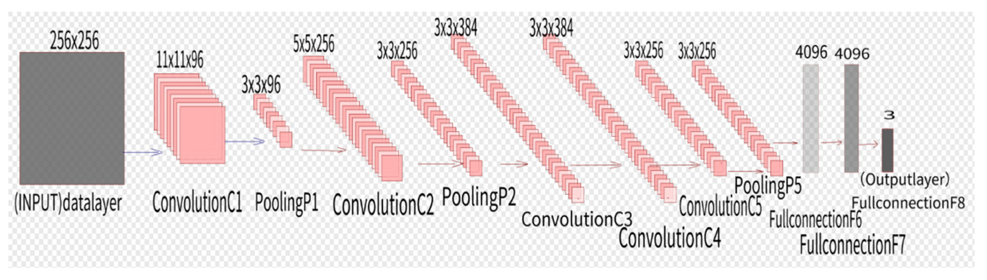
| [32] | The model is composed of an input layer, five convolutional layers, three pooling layers, and two fully connected layers. BN normalization layer is added to each layer of the model. | The lathe equipped with Siemens 840dsl CNC system is used to turn aluminum alloy 7109. Cutting speed: 220 r/min. Feed rate: 0.1 mm/r. Cutting depth: 1 mm. The CNC system collects the internal information related to the cutting force such as the spindle load, spindle torque, etc. | The recognition accuracy on the training set is 100%, the verification set is close to 89.9%, the recognition accuracy meets the requirements |
| [36] | The model is composed of an input layer, four convolutional layers, four pooling layers, one flattening layer, and two fully connected layers. The random dropout technology is applied to the flattening layer. | YG8 spiral milling. CFRP plate (material: QY9611-T700, spindle speed: 10,000 r/min, revolution shaft speed: 720 R/min, feed rate: 1 mm/s) and aluminum plate (material: TC4-DT, spindle speed: 2000 R/min, revolution shaft speed: 720 R/min, feed rate: 0.4 mm/s). Air cooling. Using mik-dji-30a and mik-dji-1a Hall current sensors to collect the current signals during processing. | The tool wear monitoring accuracy of the proposed method is 99.29% and the recall of severe wear stage is 99.60%. |
| [62] | ImageNet model is adopted and improved. The model is composed of an input layer, five convolutional layers, three pooling layers, and three fully connected layers. The initialization parameters are the best parameters trained by Caffe team, and the output is changed to three types. | The tempered steel (hrc52) was milled on a micro-CNC milling machine with double edge milling cutter (model: seco S550, diameter: 6 mm) covered with multi-layer titanium aluminum nitride coating. Maximum spindle speed: 2500 r/min. Feed rate: 1000 mm/min. A wireless triaxial accelerometer (model: m69) with sampling rate of 1 kHz/channel was used collecting vibration signal in the process of machining. | The prediction accuracy of the output is 98.05%, and the minimum loss function is 0.0353. |
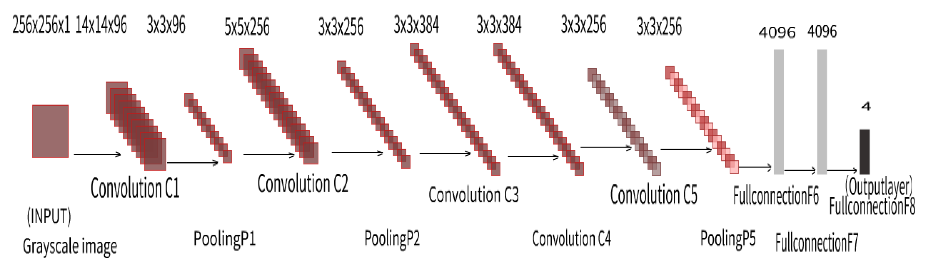
| [116] | AlexNet model is adopted and improved. The model is composed of an input layer, five convolutional layers, three pooling layers, and three fully connected layers, and the output is changed to 4 types. | Three axis vertical machining center (model: vdl-1000e), indexable face milling cutter (CVD coated carbide tool and PVD coated cemented carbide blade of Sandvik 490R Series). Cutting depth: 0.5 mm. Feed rate: 0.05 mm/Z. Linear speed: 109 m/min. Daheng image industrial digital camera (model: mer-125-30uc) was used to collect tool wear pictures. | The average recognition rate of CNN model after pre training is 96.25%, the recognition accuracy of adhesive wear is 97.7%, and the recognition rate of flank wear is 94.9%. |
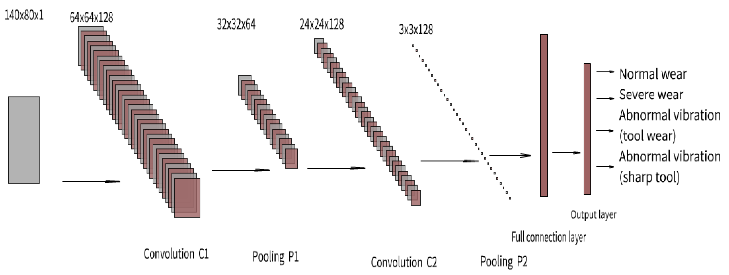
| [125] | LeNeT model is adopted and improved. The model is composed of an input layer, two convolutional layers, two pooling layers, a fully connected layer and an output layer, with 4 types of output. | Milling wear experiments were carried out on DM1007 vertical machining center under seven different working conditions. The self-built system is used to collect the vibration and current signals of the spindle, including the single-phase current signal of the spindle motor and the acceleration signal of the spindle x-direction and y-direction. The sampling frequency is 6.4 KHz. | The experimental results show that the lowest accuracy rate is 87.7%, and the highest is 92.3%. |
Publisher’s Note: MDPI stays neutral with regard to jurisdictional claims in published maps and institutional affiliations. |
© 2021 by the authors. Licensee MDPI, Basel, Switzerland. This article is an open access article distributed under the terms and conditions of the Creative Commons Attribution (CC BY) license (https://creativecommons.org/licenses/by/4.0/).
Share and Cite
Wang, Q.; Wang, H.; Hou, L.; Yi, S. Overview of Tool Wear Monitoring Methods Based on Convolutional Neural Network. Appl. Sci. 2021, 11, 12041. https://doi.org/10.3390/app112412041
Wang Q, Wang H, Hou L, Yi S. Overview of Tool Wear Monitoring Methods Based on Convolutional Neural Network. Applied Sciences. 2021; 11(24):12041. https://doi.org/10.3390/app112412041
Chicago/Turabian StyleWang, Qun, Hengsheng Wang, Liwei Hou, and Shouhua Yi. 2021. "Overview of Tool Wear Monitoring Methods Based on Convolutional Neural Network" Applied Sciences 11, no. 24: 12041. https://doi.org/10.3390/app112412041
APA StyleWang, Q., Wang, H., Hou, L., & Yi, S. (2021). Overview of Tool Wear Monitoring Methods Based on Convolutional Neural Network. Applied Sciences, 11(24), 12041. https://doi.org/10.3390/app112412041