FEM Analysis of Piezoelectric Resonator Polarization Process

Abstract

The polarization of the piezoelectric resonator depends on the direction of the applied electric field. The direction of the applied electric field is determined by the shape of the resonator and the position of the electrodes. In case of resonators with electrodes incompletely covering their bases, an inhomogeneous electric field is generated, which results in an inhomogeneous polarization of the resonator. The resonator will be polarized in some places either in a direction other than the desired one or not polarized at all. The aim of this work is to analyze the polarization process on resonators with electrodes incompletely covering their bases. The physical description is given by the linear piezoelectric equations, the Gaussian equation for the description of the electric field and by Newton’s law of force. On this basis, a FEM model is developed and used to analyze the polarization process. The results of the calculation of the electric field vector distribution are presented. Finally, the areas are identified in which polarization in the desired direction is achieved in the resonator as well as the ones where no polarization occurs.

1. Introduction

Solid solutions based on ${\mathrm{PbTiO}}_3-{\mathrm{PbZrO}}_3$, referred to as PZT ceramics, or solutions based on ${\mathrm{BaTiO}}_3$ are primarily used for the production of piezoelectric transducers. The piezoelectric properties of these materials are conditioned by the existence of spontaneous polarization. However, these samples do not show macroscopic piezoelectric properties after sintering because the directions of polarization in individual grains of the ceramics are different. Only after polarization, i.e., after application of a sufficiently strong DC electric field, and usually at increased temperatures, these macroscopically observable piezoelectric properties appear in the transducers. The efficiency of electromechanical conversion in piezoelectric transducers is assessed by the magnitude of the electromechanical coupling coefficient, which can be generally expressed as

$$k=\sqrt{\frac{W_{out}}{W_{in}}}.$$

(1)

Its square expresses the ratio of the fraction of energy $W_{out}$ that changes from electric to mechanical or vice versa to the total energy received $W_{in}$, e.g., [1].

An important factor affecting the magnitude of the electromechanical coupling coefficient is the polarization process. When an electric field of higher intensity than the so-called coercive electric field $E_c$ [2], is applied, the polarization of the piezoceramics changes in the direction of the applied electric field. The direction of the applied electric field is influenced by the shape of the piezoelectric element and the placement of the electrodes. In the case of circular resonators, the polarization field is homogeneous due to the solid electrode and the high permittivity of the piezoelectric ceramics. As a consequence, the polarization is homogeneous over the entire volume of the piezoceramic resonator.

However, there are applications, such as ultrasonic generators, where it is necessary for the supply leads to be connected to the piezoelectric element from only one side. The free side is then glued to a flexible membrane which transmits the vibrations of the piezoelectric transducer to the surroundings. In such a case, transducers with a so-called wrap-around electrode are used, as can be seen in the Figure 1.

As a result of the electrodes being wrapped around, an inhomogeneous electric field is created in the transducer. The field forms even during the polarization process. Thus, the transducer will not be polarized homogeneously in its entire volume. Some parts of the transducer will be polarized in a different direction than desired, while some parts of the transducer will not be polarized at all. This fact causes different operating characteristics of the piezoelectric element than expected, e.g., a lower electromechanical coupling factor.

Relevant publications dealing with similar issues include [3,4,5,6,7,8,9,10,11]. The effect of polarization is studied in these works, either by analytical methods due to the significantly simpler geometry [9], experimentally [11], or using the finite element method [3,4,5,6,7,8], however, always in a configuration or application different from the one presented here.

In piezoelectric ceramics, nonlinear phenomena are also present in the elastic, piezoelectric and dielectric spheres. As an example, phenomena on domain walls can be mentioned. For simple configurations of several domain walls, these are studied analytically, e.g., in [12,13], and experimentally, e.g., in [14]. Phenomena at domain walls have been studied by the author in [15,16].

Neglecting of nonlinearities, lattice effects, grain boundaries, self-polarization, etc. would not be possible in the case of analysis of polarization phenomena on a microscopic scale, at the level of individual domain interfaces. On a macroscopic scale, in terms of the macroscopic properties of the piezoelectric element, a linear model is used in publications [3,4,5,6,7,8] to determine the direction of polarization in the piezoelectric ceramic.

Leaving aside the above-mentioned publications devoted to the analysis of phenomena at a maximum of several domain walls, so far only works computationally affecting only linear phenomena involved in the process of polarization have been published. The reason is the challenging implementation of nonlinear equations into a mathematical model and at the same time and in orders of magnitude higher computational cost. This is due to the implementation of the nonlinear model itself, but especially due to the need to take into account the number of domain walls in a real piezoelectric element. Considering the number of domain walls contained in a real piezoceramic resonator, such a model would not be computationally feasible.

Therefore, computational methods can only realistically capture linear phenomena, as shown in [3,4,5,6,7,8]. Here, however, the computational model is used in different applications, in the study of electric field distribution using a spherical polarizing electrode [3], and to determine the material polarization level in a porous piezoelectric material [4,5,6,7,8]. None of the available publications has so far been devoted to the study of the process of polarization of piezoelectric elements with asymmetric electrodes, and no work has yet presented the approach used by the author to simulate the process of polarization.

2. Materials and Methods

The presented approach is based on the numerical model of the problem, based on the physical description of piezoelectric continuum, see [17,18]. Such a description includes elastic Equations (2), electric Equations (3) and state equations for piezoelectric material (4) and (5), relation between electric field and potential (6), relation between strain and mechanical displacement (7).

$$\nabla ·\mathbf{T}=\frac{\partial {\mathrm{T}}_{\mathrm{ij}}}{\partial x_j}=0i,j=1,2,3x\in \Omega ,$$

(2)

$$\nabla ·\mathbf{D}=\frac{\partial {\mathrm{D}}_{\mathrm{j}}}{\partial x_j}=0$$

(3)

$${\mathrm{T}}_{\mathrm{ij}}=c_{ijkl}·{\mathrm{S}}_{\mathrm{kl}}-e_{ijk}·{\mathrm{E}}_{\mathrm{k}},i,j=1,2,3.$$

(4)

$${\mathrm{D}}_k=e_{kij}·{\mathrm{S}}_{\mathrm{ij}}+{\epsilon }_{kj}·{\mathrm{E}}_{\mathrm{j}}+{P_k}^s,k=1,2,3,$$

(5)

$$E_i=-\frac{\partial \phi }{\partial x_i},$$

(6)

$$S_{ij}=\frac{1}{2}\left(\frac{\partial u_i}{\partial x_j}+\frac{\partial u_j}{\partial x_i}\right),$$

(7)

where T, D, S, E, u, ${P_k}^s$, c, e and $\epsilon$ are stress, the vector of electric displacement, strain, electric field, mechanical displacement, spontaneous polarization and material tensors. $\Omega$ denotes the volume of sample. The FEM-solution of this problem [17,18], leads to the set of linear equations with large and sparse matrices,

$$\left(\begin{array}{cc}\mathbf{K}& {\mathbf{P}}^{\mathrm{T}}\\ \mathbf{P}& \mathbf{E}\end{array}\right)\left(\begin{array}{c}\mathbf{U}\\ \Phi \end{array}\right)=\left(\begin{array}{c}{\mathbf{R}}_{\mathbf{U}}\\ {\mathbf{R}}_{\Phi }\end{array}\right),$$

(8)

where $\mathbf{K},\mathbf{P},\mathbf{E},\mathbf{U},\Phi ,{\mathbf{R}}_{\mathbf{U}},{\mathbf{R}}_{\Phi }$ are elastic, piezoelectric and electric part of global matrix, displacements and potentials in nodes of finite element mesh and vector of right hand side, which contains boundary conditions. These variables allow to compute the elastic stress, electric field, electric displacement and energies.

2.1. Simulation of the Polarization Process

A crucial step in the development of the model is to take into account the material properties of the real piezoceramic resonator. As already stated, the subject of the simulation is the very event of polarization of the transducer. Let us begin with the fact that before the polarization process starts, the transducer is macroscopically non-piezoelectric. That is due to the different orientation of the individual ceramic grains.

At the level of the finite element method model, it is not possible to work with geometrically simpler and smaller entities than the individual finite elements, the set of which approximates the volume of the piezoelectric transducer. According to [19], the grain size of PZT type piezoelectric ceramics is in the range (1–10) $\mathsf{\mu }\mathrm{m}$. Piezoelectric transducers typically have a diameter in the range of (1–5) cm and a thickness in the interval of (0.5–5) mm.

If we consider a piezoelectric transducer with a diameter of 20 mm, thickness of 2 mm, ceramic grain size of 5 $\mathsf{\mu }\mathrm{m}$, the discretization will contain the number of nodes in the order of ${10}^9$. Outside of the nodes where the Dirichlet boundary condition is specified, we determine four degrees of freedom, three components of the displacement vector and the electric potential. The resulting set of algebraic equations will therefore have a dimension four times the number of discretization nodes. Such a system of equations is already at the verge of solvability on a common computing station and in acceptable time (within a time frame of max. tens of minutes).

As stated above, the model considers only linear phenomena, omitting nonlinearities that arise from the existence of domain interfaces. Therefore, we do not have to consider domain interfaces in the model. We perform the analysis of the electric field distribution to determine the areas in which polarization occurs in the resonator, resp. polarization in the direction identical to the thickness of the transducer, which is the direction that has a fundamental effect on the electromechanical coupling coefficient of the thickness oscillation. The model must therefore capture the distribution of the electric field well enough, especially in areas where the field will be inhomogeneous, i.e., in the area where the electrodes wrap around. This can be achieved by adjusting the discretization parameter, by refining the finite element mesh, in the mentioned areas.

Based on the above stated facts, it can be assumed that the model will not contain the same number of elements as there are in a real ceramic grain transducer. We replace the random orientation of the individual grains with a random orientation of the material property tensors in the individual finite elements of the model. We will treat each element as a grain of ceramics and assign it material tensors transformed into a randomly chosen Cartesian coordinate system. This idea is implemented by the program code in the following way:

1.

Define the coordinate systems into which the material tensors will be transformed. Thirty-six coordinate systems were created, derived from the basic Cartesian coordinate system of rotations about the x-coordinate axis ($x_1$) in 10${}^{\circ }$ increments. That is, rotations of 0${}^{\circ }$, 10${}^{\circ }$, 20${}^{\circ }$ ...350${}^{\circ }$. In each rotation around the coordinate axis x, create 35 more coordinate systems, rotating about the axis y ($x_2$) by 10${}^{\circ }$, i.e., rotations by 10${}^{\circ }$, 20${}^{\circ }$ ...350${}^{\circ }$. We have 36 × 36 = 1296 coordinate systems in total.

2.

Using transformation equations, e.g., [20], transform material tensors into a specified coordinate system. The material tensors are transformed into the coordinate systems defined inpoint 1. In the case of piezoelectrics, these are tensors of elastic modules, piezoelectric coefficients, permittivity.

3.

Assign a unique identifier to the transformed material constants that refers to the material properties. This is essentially a pointer to a structure that carries information about the actual values of the material constants and about the coordinate system into which the material constants have been transformed.

4.

Give the individual finite elements their material properties using the identifiers specified in the previous section. Using a pseudo-random number generator, numerically labeled finite elements are selected, to which individual material property identifiers are gradually assigned.

Thus, we have a total of 1296 sets of material tensors differing in the orientation of the z ($x_3$) axis, which determines the direction in which the polarized part of the ceramics is oriented depending on the direction and magnitude of the applied electric field. Here we make another simplifying assumption, with the following consequences:

• We have a finite set of polarization directions that will not always exactly match the direction of the calculated polarization field. However, a deviation of 5${}^{\circ }$ from the calculated direction of polarization will be considered acceptable.
• Each coordinate system created by rotating the basic Cartesian coordinate system about the x and y axes is unique. We no longer rotate about the z-axis. This rotation is unnecessary because piezoelectric ceramics have a type of crystal symmetry [21], which implies transverse isotropy of material properties. That is identical properties in the $zx$ and $zy$ planes and different properties in the $xy$ plane, i.e., in the plane perpendicular to the polarization direction [22].
• We consider 1260 directions of possible polarization versus the number of directions of polarization of the individual ceramic grains in the transducer, which will be of the same order as the number of ceramic grains contained in the transducer. However, if we consider the number of elements in the model to be of the order of ${10}^3$–${10}^4$, then each of the 1260 material sets defined will occur in the model at most of the order of ${10}^2$. Respectively, each material property will occur on average once in the randomly selected 1260 elements. Even this circumstance is acceptable; from a physical point of view, it does not significantly affect the quality of the achieved result.

Transformed material properties, represented by their numerical identifiers, should not be assigned to the individual finite elements sequentially. Given the numbering of elements in a finite element network, we would arrive at a certain form of periodicity of the assignment of material properties. For this reason, a pseudo-random number generator is used in point 4 of this algorithm.

2.2. Boundary Conditions

The boundary conditions correspond to the real polarization conditions. The resonator is held in its center by removable power supply leads. Thus, the Dirichlet boundary condition $u_x=u_y=u_z=0$ is given on the bottom side at the mounting location, and the Dirichlet boundary condition $u_x=u_y=0$ is given on the top side. At the top electrode, the transducer is not fixed in the thickness direction (z-axis) because the temporary power supplies are not ideally rigid. The transducer is not mechanically stressed during the polarization process, and the homogeneous Neumann condition $\mathbf{T}·\mathbf{n}=0$ is entered on the remaining edge.

The wrap-around electrode is grounded, i.e., the electrical potential of the electrode is 0 V. A polarization voltage, the electric potential ${\phi }_p$ is applied to the top electrode. Homogeneous Neumann condition $D_N=0$ is given on the remaining surface of the transducer (not covered by the electrodes). This boundary condition can be entered due to the fact that the permittivity of piezoelectric materials reaches orders of magnitude ${10}^2$–${10}^3$ times higher than the permittivity of air or silicone oil [23], in the bath of which the polarization takes place. At constant electric field strength, electrical induction is directly proportional to the magnitude of the permittivity. At the interface of two materials with significantly different permittivities, the electrical induction will be higher in the ratio of the permittivities in an environment with higher permittivity. The component of the electric induction vector perpendicular to the material interface (the normal component) will be negligible in such a case.

2.3. Polarization Process

The polarization process itself is simulated as follows. Gradually, with the step ${\phi }_k/n$, in the interval $〈0,{\phi }_k〉$ the voltage on the top electrode is increased in the model. In each step

• the evaluation of each element is performed to see whether the magnitude of the coercive electric field ($E_c$) is exceeded,
• if the magnitude of the coercive field on the element is exceeded, it is assigned material properties whose z axis of the transformed coordinate system has the direction closest to the direction of the calculated electric field on the element.

In practice, the Euclidean norm of the difference between the unit vector of the electric field direction and the unit vector of the z-axis direction of each transformed coordinate system is calculated. Polarization causes an orientation [1], that corresponds to the orientation of the z-axis in the direction of the polarization field.

In each step of the calculation, we get

• information about the number of elements in which the polarization occurred,
• information about their spatial location,
• from the knowledge of the polarized elements and the knowledge of their volumes, the volume of polarized material in the transducer can be calculated.

2.4. Task Assignment

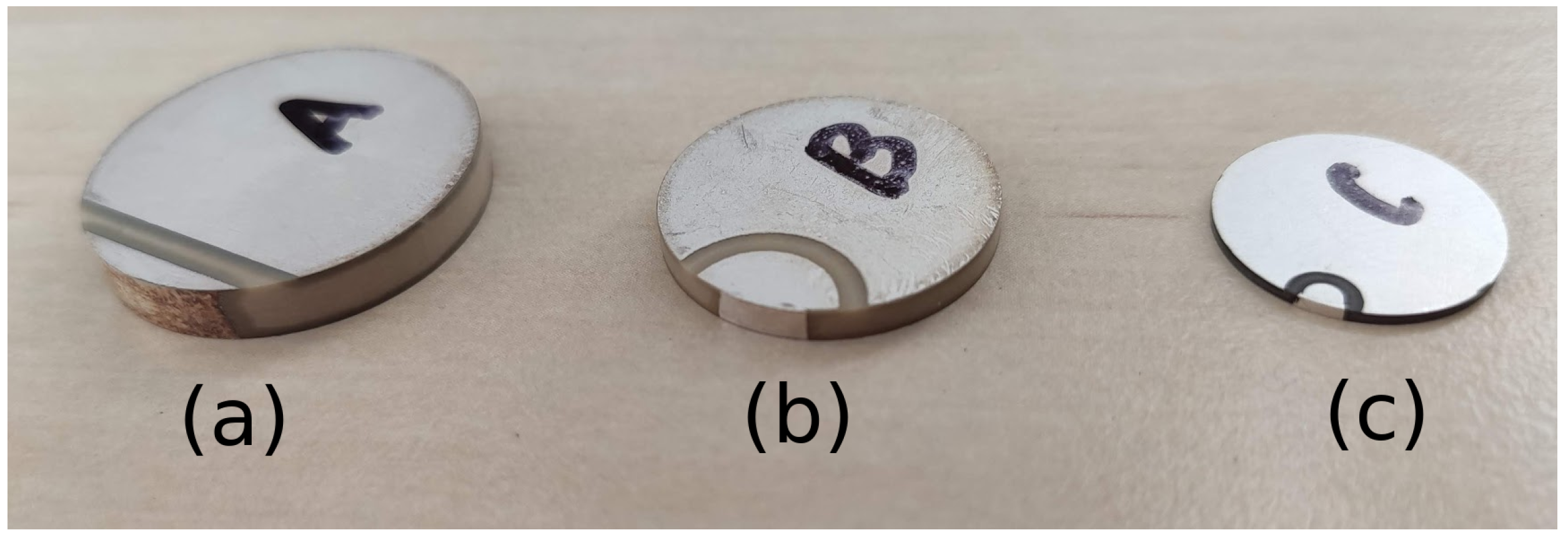
This approach is applied when comparing the polarization of two types of piezoelectric transducers, labeled (a) and (b), shown in Figure 1. The transducers differ in the shape of the electrode wrap-around. In case of (a), the overlay is in the shape of a circular segment, in case of (b), it is in the shape of intersecting circles.

The polarization of the transducer will be analyzed in relation to the shape of the electrode wrap-around. To make the results comparable, we will consider both piezoelectric transducers of the same size. The criterion of equivalence for the wrap-around electrodes needs to be established. We will consider equivalent the electrodes that will have the same area of wrap-around electrode in both cases.

2.4.1. Geometric Characteristics

Let $\alpha =d/t$, where d is the diameter of the disk and t its thickness. For circular resonators with dimension ratio in the range $1<\alpha <10$, there is no mode in the spectrum of natural oscillations that could be called a basic thickness resonance, a basic thickness mode of the oscillation. There is a strong coupling of thickness and radial oscillations in the spectrum, which is due to the comparable sizes of diameter and thickness, [21].

Therefore, we will consider a disk with a dimensional ratio of $\alpha \gg 1$, where the basic thickness mode of the oscillation is significantly distinct. The thickness mode of oscillation is used in electroacoustic and ultrasonic transducers. In them, we find electrodes in the studied configuration-electrodes are wrapped from one base to another.

In the monograph [21], chapter 5.3, the frequency spectrum of a resonator with entire electrodes on both circular surfaces with ratio $\alpha =23.7$, made of NCE51 piezoelectric ceramics, is analyzed. The $\alpha$ ratio is therefore suitable to excite the basic thickness mode of the resonator. We will thus work with a resonator that maintains the dimensions of resonator from chapter 5.3 of the monograph [21], except that it will not be fully electroded on both circular surfaces. The bottom electrode will be considered wrapped-around

(a)

in the shape of a circular segment,

(b)

in the shape of an intersection of circles.

A diagram of the dimensions of the transducers is shown in the Figure 2. The dimensions of the transducers are given in the

Table 1. Dimensions of the transducers.

d (mm)	47.9	t (mm)	2.02
$s_1$ (mm)	4.66	$r_1$ (mm)	9.50
$s_2$ (mm)	2.00	$r_2$ (mm)	7.50

.

The dimensions of the wrap-around are chosen so that the area of the wrapped around electrodes is identical in both cases. The ratio of the wrap-around to the total circular area is approximately $1/25$.

2.4.2. Material Characteristics

We consider the transducers made of NCE51 piezoelectric ceramics, again in accordance with Chapter 5.3 in [21]. NCE51 ceramics has a hexagonal symmetry class of 6 mm. This fact is reflected in the form of the material tensors. For the hexagonal symmetry class 6 mm, the permittivity tensors of piezoelectric modules and elastic modules have the following structure

$$\epsilon =\left(\begin{array}{ccc}{\epsilon }_{11}& 0& 0\\ 0& {\epsilon }_{11}& 0\\ 0& 0& {\epsilon }_{33}\end{array}\right),$$

$$\mathbf{e}=\left(\begin{array}{cccccc}0& 0& 0& 0& e_{15}& 0\\ 0& 0& 0& e_{15}& 0& 0\\ e_{31}& e_{31}& e_{33}& 0& 0& 0\end{array}\right),$$

$$\mathbf{c}=\left(\begin{array}{cccccc}{c}_{11}& c_{12}& c_{13}& 0& 0& 0\\ c_{12}& c_{11}& c_{13}& 0& 0& 0\\ c_{13}& c_{13}& c_{33}& 0& 0& 0\\ 0& 0& 0& c_{44}& 0& 0\\ 0& 0& 0& 0& c_{44}& 0\\ 0& 0& 0& 0& 0& c_{66}\end{array}\right).$$

From the structure of material tensors, from the equality of some of their elements, the property mentioned in the Section 2.1, i.e., the transverse isotropy of piezoelectric ceramics, is also evident. The values of the elements of the above-mentioned tensors are given in the

Table 2. Material properties of NCE51 ceramics.

${\epsilon }_{11}^S\left(1\right)$	906	$c_{12}^E$$\left(\mathrm{Pa}\right)$	$8.26·{10}^{10}$
${\epsilon }_{33}^S\left(1\right)$	823	$c_{13}^E$$\left(\mathrm{Pa}\right)$	$8.85·{10}^{10}$
$e_{31}$$(\mathrm{C}/{\mathrm{m}}^2)$	$-4.80$	$c_{33}^E$$\left(\mathrm{Pa}\right)$	$17.2·{10}^{10}$
$e_{33}$$(\mathrm{C}/{\mathrm{m}}^2)$	$17.2$	$c_{44}^E$$\left(\mathrm{Pa}\right)$	$2.04·{10}^{10}$
$e_{15}$$(\mathrm{C}/{\mathrm{m}}^2)$	$13.7$	$c_{66}^E$$\left(\mathrm{Pa}\right)$	$2.30·{10}^{10}$
$c_{11}^E$$\left(\mathrm{Pa}\right)$	$12.9·{10}^{10}$	$\varrho$$(\mathrm{kg}/{\mathrm{m}}^3)$	7850
$E_c$ (kV/mm)	$0.95$	$E_s$ kV/mm	3

and are taken from [21,24]. In the table, permittivity is given as relative permittivity.

The table also shows the density value of the given material, the value of the coercive electric field ($E_c$) and the value of the maximum applicable electric field as recommended by the manufacturer. The latter can be understood as the minimum value of the dielectric strength of the material, as described in the introduction. It should be noted that the orientation of the crystal system and the labeling of the components of the material tensors are in accordance with the [25] standard.

2.4.3. Geometry and Finite Element Mesh Generation

Due to the symmetry of both transducer variants, the problem can be solved as symmetric. The plane of symmetry is the plane A-A${}^{\prime }$ or B-B${}^{\prime }$ according to the diagram in Figure 2. The geometry of the model will therefore be formed by one symmetric half of the transducer. The other symmetric half will be replaced by entering the appropriate boundary conditions.

The geometry created by the GMSH software, see [26], can be seen in the Figure 3.

In the geometry file, physical entities are defined. These combine the geometric surfaces that make up each electrode. Boundary conditions will be further specified for these physical entities. The finite element mesh defined on the created geometry is shown in Figure 4.

The mesh is smoothed around the edges of the wrapped-around electrodes. Significant changes in the electric potential gradient can be expected at these locations. In each case, the mesh consists of

(a)

9676 nodes, 44,780 tetrahedral elements,

(b)

9298 nodes, 43,546 tetrahedral elements.

The discretization parameter was set identically on the equivalent geometric entities in both cases, the number of nodes and elements differs due to the different geometry in the area of the wrapped-around electrode.

2.4.4. Calculation of the Polarization Process

The values of the magnitude of the coercive electric field and the dielectric strength, Table 2, are the decisive parameters for the simulation of the polarization process. According to the procedure described in Section 2.3, the electric field will be applied to the transducer through the electrodes in the interval $〈0,3〉$ kV/mm

• in steps of 0.2 kV/mm in the interval $〈0;0,8〉$ kV/mm,
• in steps of 0.05 kV/mm in the interval $〈0,8;1,3〉$ kV/mm,
• in steps of 0.2 kV/mm in the interval $〈1,3;3〉$ kV/mm.

The electric field will be entered through the Dirichlet boundary condition on the surfaces representing the electrodes, as described in the Section 2.3. The Dirichlet condition implies the input of a known electric potential. The relationship between the electric field strength and the electric potential is given by the Equation (6). If we consider the wrapped-around electrode to be grounded, the electric potential at the opposite electrode can be expressed as

$${\phi }_D=E_{app}t,$$

(9)

where $E_{app}$ is the electric field we want to apply to the transducer and t is the thickness of the piezoelectric transducer.

The boundary condition in the plane of symmetry will have the value

$${\mathrm{D}}_{\mathrm{k}}{n}_k={\mathrm{D}}_{\mathrm{N}}=0,$$

(10)

where $\mathrm{D}$ is the electric induction vector, $n_j$ is the j-th component of the unit vector of the outer normal to the plane of symmetry. The induction flux across the surface in the plane of symmetry is therefore zero.

Before starting the calculation, material properties will be assigned to each element according to the procedure given in Section 2.1. In each step, it will be evaluated in which elements the coercive electric field has been exceeded. According to the procedure from Section 2.3, the material properties will be modified in these elements according to the direction of the calculated field.

3. Results

Figure 5 shows the calculated electric potential for $E_{app}=1$ kV · mm${}^{-1}$. Since the entered Dirichlet boundary condition varies only in size, not in the area on which it is specified, the nature of the electric potential distribution in the transducer is the same for any value of boundary condition.

Figure 6 shows the calculated electric potential for $E_{app}=1$ kV · mm${}^{-1}$ in sections A-A’ resp. B-B’ according to the diagram shown in Figure 2. A linear progression of the magnitude of the potential between the electrodes is observed in the region where the electrodes are opposite. In the place of the wrapping-around, the potential is zero due to the identical potential of the electrodes on both circular surfaces.

Figure 7 shows the magnitude of the electric field strength for $E_{app}=1$ kV · mm${}^{-1}$. A homogeneous electric field is observed in the area where the electrodes are opposite. A zero value of the electric field intensity is evident in the areas where the lower electrode is wrapped-around. In this area there will be no polarization of the transducer. Inhomogeneities occur in the area between the edges of the wrapped-around electrode and the electrode covering only the top circular part of the transducer.

The same statement applies here as for the calculated electric potentials. The given Dirichlet boundary condition varies only in its magnitude, not in the area over which it is specified. The character of the electric field intensity distribution is the same for any size of $E_{app}$, differing only in the magnitude of the electric field intensity vectors. This visualization of the calculated electric field strength distribution provides only qualitative information about the conditions that occur during the polarization process.

The correctness of the simulations can be verified by comparison with the results in [4], where the piezoelectric coefficient $d_{33}$ is determined and compared with experimentally achieved valueS. The coefficient $d_{33}$ is directly related to the direction of polarization, in direct relation to the volume polarized in the direction of the resonator thickness. In paper [4], a conceptually identical model was used to determine the coefficient $d_{33}$ and its value was verified experimentally. The relevance of the results presented here can be based on the above.

4. Discussion

The result of a quantitative nature, which indicates the conditions during polarization, is the graph in the Figure 8.

The graph shows the dependence of the polarized volume of the transducer on the magnitude of the polarization electric field for both variants of the analyzed transducers. A significant increase in the polarized volume occurs when the magnitude of the coercive field in the area between the opposite electrodes is reached. The polarized volume of the transducer is about 1.2% higher in the case of variant (b) compared to variant (a). This difference can be explained by the difference in the volume occupied by the wrap-around area, including the area below the gap between the electrodes. This difference is about 1% higher in the case of variant (a) compared to variant (b). The further increase after exceeding the coercive electric field between the opposite electrodes occurs very slowly, in the vicinity of the wrapped-around electrode.

The graph in Figure 9 shows the dependence of the volume polarized in the thickness direction of the transducer on the magnitude of the polarization field $E_{app}$. In the case of variants (a) and (b), the volume polarized in the thickness direction is clearly lower than the total polarized volume of the transducers. An interesting result can be seen in the interval (0.8–0.9) kV/mm of the polarization field. In this interval, an increase in the polarized total volume is evident from the graph in Figure 8, whereas in the graph in Figure 9, which shows the dependence of the volume polarized in the thickness direction, this increase is not apparent.

We can therefore hypothesize that polarization occurs in the interval (0.8–0.9) kV/mm in directions different from the direction perpendicular to the thickness. This hypothesis is consistent with the fact that the gap between the electrodes is slightly smaller than the thickness of the transducer, see Table 1. The polarization of the material in the area of the gap between the electrodes will therefore occur at a lower voltage difference between the electrodes, and thus in a direction different from the direction perpendicular to the thickness than in the direction of the transducer thickness, between the opposite electrodes. It stems from the relation (9); the magnitude of the electric field intensity is inversely proportional to the distance between the electrodes.

The macroscopically piezoelectric area, which is effective in terms of electromechanical response, is precisely the area polarized in the direction of the transducer thickness. That is, as would be achieved with a circular resonator that is fully electroded on both sides. It is clear from the graph in the Figure 9 that

• 88% resonator volume in configuration (a),
• 90% resonator volume in configuration (b)

is effective in terms of electromechanical transformation, and therefore also in terms of the coefficient of electromechanical coupling.

The remaining 10% or 12% respectively of the resonator are polarized either in a direction different from the direction perpendicular to the circular surfaces or not polarized at all. The most prominent area that is not polarized is the part covered by the wrapped-around electrode. Configurations (a) and (b) are two possible designs differing in the shape of the wrap-around electrode. Based on the comparison of the results for both designs, it can be stated that the design of the wrap-around electrode does not significantly affect the volume polarized in the thickness direction of the resonator.