Automatic Crack Classification by Exploiting Statistical Event Descriptors for Deep Learning

Abstract

In modern building infrastructures, the chance to devise adaptive and unsupervised data-driven structural health monitoring (SHM) systems is gaining in popularity. This is due to the large availability of big data from low-cost sensors with communication capabilities and advanced modeling tools such as deep learning. A promising method suitable for smart SHM is the analysis of acoustic emissions (AEs), i.e., ultrasonic waves generated by internal ruptures of the concrete when it is stressed. The advantage in respect to traditional ultrasonic measurement methods is the absence of the emitter and the suitability to implement continuous monitoring. The main purpose of this paper is to combine deep neural networks with bidirectional long short term memory and advanced statistical analysis involving instantaneous frequency and spectral kurtosis to develop an accurate classification tool for tensile, shear and mixed modes originated from AE events (cracks). We investigated effective event descriptors to capture the unique characteristics from the different types of modes. Tests on experimental results confirm that this method achieves promising classification among different crack events and can impact on the design of the future of SHM technologies. This approach is effective to classify incipient damages with 92% of accuracy, which is advantageous to plan maintenance.

1. Introduction

The aim of structural health monitoring (SHM) is to achieve efficient and cost-effective structural reliability and sustainability through integrated health management and prognosis. The area of the SHM receiving most attention in the literature [1,2,3,4,5,6,7,8,9] is related to the extraction of data features allowing to distinguish between the undamaged and damaged structures.

The continued growth of internet-of-things (IoT) and digital twin has brought many new sensing mechanisms suitable for SHM. In particular, acoustic emission (AE) monitoring [10,11] is becoming an established method for feature extraction. It is based on the simultaneous analysis of multiple parameters, such as vibration amplitude and frequency, with the characteristics of acoustic wave as originated during a crack. AE signals are usually investigated using the moment tensor analysis (MTA) [12] and/or the calculation of AE parameters [2]. AE parameters, such as average frequency (AF), rise time (RT), duration (DUR), rise angle (RA), peak amplitude as well as energy (ENE), have been shown to be effective to classify both tensile and shear failures [2,8,13,14,15,16,17]. During solicitations, it is well known that the propagation distance of the acoustic wave and the quality of the propagation path (i.e., presence of defects, air gaps) have an impact on the calculation of AE parameters, such as AF and RA [6,18], especially in the presence of damage [4]. However, there is no such consolidated procedure for the identification of mixed-mode events [19] occurring mostly at the transition from a regime having mainly tensile crack events to the other characterized by the majority of shear crack events. A recent study [14] has pointed out that data quality can be compromised by untreated disturbances related to the measuring system (i.e., the sensor-induced distortion) or the environment (e.g., scattering attenuation due to damage accumulation, viscous damping, inhomogeneity of concrete, structural defects of internal specimen, etc.). Therefore, those disturbances should be carefully taken into account and minimized [10,20] for reliability.

Recently, alternative AE classification studies using machine learning (ML) have been proposed in the literature. Some of them use a combination of wavelets and specialized ML techniques for classification, such as random forests [21], or support vector machine (SVM) [22,23] achieving 84.7% and 89.4% of accuracy, respectively. ML applications in the prediction of structural performance have been presented [24], demonstrating the potential, usefulness and feasibility of these techniques once applied on SHM systems. Kim and coworkers [25] have proven how artificial neural network (ANN) combined with principal component analysis (PCA) can be promising for binary classification of AE signals from wood drying. Li and coworkers have used K-means clustering [26] of stainless steel by focusing on the analysis of frequency bands in AE signals. A convolutional neural network (CNN) was implemented by [27] to recognize dispersion curves on the spectrograms of AE signals or identifying different vehicle engines [28] rather than crack events. In bridge engineering, a binary classification problem has been successfully analyzed using CNNs to recognize noise and fracture AE signals [29]. These contributions clearly show the promising results either in terms of classification and remaining fatigue life prediction as well as in status-driven AE monitoring capabilities.

Here, we describe a procedure to address the above cited problems in order to achieve both automatic and robust classification of crack events in AE data. In our work, we consider different statistical operators, i.e., instantaneous frequency, spectral entropy and spectral kurtosis, which have already been effective for characterizing a variety of non-stationary signals [30,31] as the inputs of a deep learning (DL) neural network. Instead of applying DL methodology to image input data of concrete surfaces [32,33], in this paper, we use DL to classify different AE solicitations represented by time varying signals.

The chance to properly characterize the temporal behavior of AE events using DL depends on the type of information that contributes to the learning process. For example, traditional AE parameters, which generally provide a single number as a result (e.g., AF, RA, ENE), are not a favorable choice for feeding a DL network because they cause an increase in the learning time and decrease in the overall performance [34].

Temporal series classification is a standard analysis problem, which requires the identification of a functional dependence between the set of possible time series and the finite number of classes using a training set with labeled results. There are several works illustrating that DL is suitable for classification problems and can outperform other algorithms [35,36] which encourage further work in this direction. DL models exist, such as recurrent neural networks (RNNs), that are designed specifically for processing sequential data, and thus could be applied for time series.

Here, we have built an RNN model constituted of bidirectional long short-term memory units (Bi-LSTM) [37] to properly classify different classes of crack events. The main motivation for this choice is that Bi-LSTMs are: (i) easier to train than RNNs [38], (ii) effective in the classification and prediction of time-series [34], and (iii) capable of learning long-term dependencies [39,40]. The performance of the DL neural network is evaluated on a dataset of AE measurements and compared against other DL-based techniques in terms of classification accuracy. Furthermore, results are comparable to other achievements [41,42,43] when applying DL to detecting faults in rotating machinery. Notably, an additional benefit of our framework is that it can be embedded into SHM systems for the lifetime monitoring of large-scale structures. The paper is organized as follows. Section 2 provides information about the acquisition system and the experimental setup. Section 3 describes the proposed framework. Section 4 presents results and the discussion followed by conclusions provided in Section 5.

2. Multi-Sensors Acquisition System and Experimental Setup

The AE-based methodology relies on the investigation of the elastic energy as generated from a crack formation. In concrete, the standardization procedure for the characterization of AE data is active [44], aiming at proposing a well-established setup for sensors and measurement protocols. With regard to this, previous studies [45,46] have proposed a multi-triggered acquisition system (AS), which takes into account emerging standards, enabling both high sampling frequencies and reduced storage requirements. Such types of AS are attracting a growing interest and becoming widespread [10,47,48] to modern infrastructure with long service life. Specifically, for the setup used here (Figure 1a–c), an asymmetric arrangement [46] of five AE transducers has been used; Figure 1d illustrates a representation of the acquisition system with a sketch of the sensors layout S1–S5). Signals from all transducers are pre-amplified by 40 dB, digitized and collected by a multi-channel system. Each channel (Ch1–Ch5) is directly coupled to a single sensor (S1–S5). The software, in cooperation with the acquisition board, automatically triggers the recording of such relevant events [49].

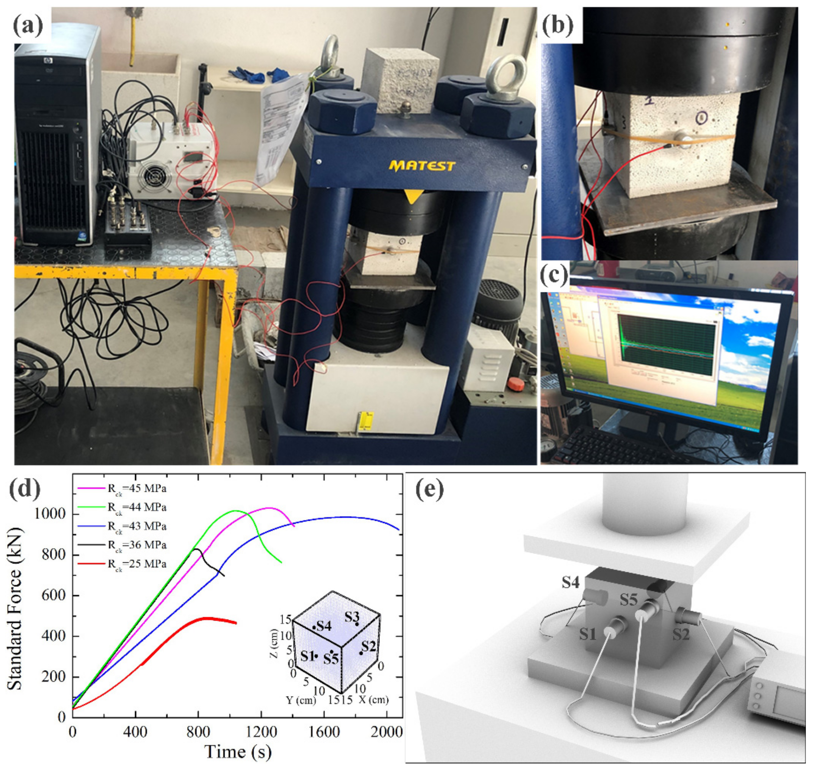
2.1. Experimental Setup

As shown in Figure 1a–d, the experimental setup consists of:

• One hydraulic press with a closed loop governing system with 5000 kN connected to the AS to control and record the load-displacement diagram;
• Piezoelectric transducers, R15α, with a peak sensitivity of 69 V/(m/s), resonant frequency 150 kHz, and directionality ±1.5 dB [50];
• Controlling hardware appliance constituted by multiple Logic Flat Amplifier Trigger generator (L-FAT) and DAta acQuisition boards (DAQ) NI-6110 with four input channels each, 12-bit resolution, and sampling frequency f_AS = 5 Msample/s wherein a channel (Ch) is directly associated to each transducer.

A complete description of the acquisition system can be found in [46]. The experimental tests were conducted on a set of concrete cubic specimens with dimension 15 × 15 × 15 cm³ without any steel reinforcement. Such specimens were cured for 28 days with temperature 20 ± 2 °C and relative humidity equal to 95% according to the norm UNI EN 12390-3:2009 [51]. The concrete specimens were realized by a specialized Company. The chosen specimen granulometry is the one typically used for civil constructions. The granulometry distribution was obtained in accordance with the Fuller curve [52] characterized by maximum dimension of the aggregate equal to 20 mm. The company furnished the specimens with surface planarity tolerance of 0.05 mm of the faces that will be in contact with the press test machine. The specimens were classified following [51], ranging between C20/25 and C35/45. In particular, the first number of the class is the cylinder compressive strength in MPa and the second is the cubic one.

2.2. Experimental Tests

The AE transducers were arranged along the vertical sides of the specimen [46]. After calibration, we investigated 50 specimens having different compressive strengths, R_ck, ranging from 25 up to 45 MPa (cylinder/cube compressive strengths). The compression tests were carried out on the cubic specimens, after the curing phase and according to UNI EN 13477-2:2011 [53]. The load was applied to one face using uniaxial compression, while the other ones were maintained fixed. The constant displacement rate was 0.1 mm/min [54] until failure. Figure 1d provides some of the experimental compression load curves obtained for the concrete specimens, whereas Figure 1e depicts a sketch of the acquisition system. All the corresponding load curves are characterized by an elastic regime (linear region) with the maximum at the peak load (inflection point) [55]. After crossing that point, the material deformations become irreversible (plastic regime) and the non-linear response indicates that the sample is significantly damaged and close to the collapse [46,56]. During the compression test, the AE events were detected, collected and processed to be used for DL training and testing purposes. The measurement dataset is available online (see Supplementary Materials).

3. Framework for the Real-Time Classification of Acoustic Emission Data

Figure 2 shows the schematic block diagram of the processing pipeline. It comprises a number of waveform preprocessing blocks [46] performing: (I) transducer’s transfer function removal (TFR), (II) Hilbert–Huang transform (HHT) and (III.1) feature extraction. Once preprocessed, the output data feed the (III.2) DL-based [46,57] processing block used for the classification of AE signals. From a given input, each block on the pipeline performs different I/O operations and it is numbered according to sequential tasks. In the waveform preprocessing blocks, any raw transducer time-domain measurement $r_{b,q}\left(t\right)$ related to the q-th AE (q = 1…Q) captured from the b-th channel (b = 1…5 in our system) is processed through blocks from (I) to (III.2). In (I), $r_{b,q}\left(t\right)$ is deconvoluted using TFR [10] with the sensing acquisition system, thus generating a reconstructed signal $s_{b,q}\left(t\right)$. Then in (II), $s_{b,q}\left(t\right)$ is processed by means of the HHT [58], in order to perform denoising and detrending, generating refined signal ${\tilde{s}}_{b,q}\left(t\right)$. Subsequently, we have evaluated, against all the available channels, the solicitation having the highest energy E, ${\widehat{s}}_q\left(t\right)$, such that ${\widehat{s}}_q\left(t\right)=\underset{b}{\max }\left\{E_{{\tilde{s}}_{b,q}}\right\}$. ${\widehat{s}}_q\left(t\right)$ is then used to feed the next block of the pipeline.

In block (III.1), for a given q-th AE, we have extracted different statistical properties (described in Section 3.2 and

Table 1. Summary of the statistical properties used in this study. We generally refer to these functions as event descriptors (EDs).

Function	Acronym	Domain	Expression	Description	Ref.
Instantaneous Frequency	IF	Time	$IF\left(t\right)=\frac{1}{2\pi }\frac{d\varphi }{dt}$	Derivative of the phase of the analytic signal of the input	[73,74]
Spectral Entropy	SE	Freq.	$\begin{array}{l}SE\left(f\right)=\\ -\frac{{\displaystyle \sum _{m=1}^{M}PDF\left(m\right){\log }_2\left(PDF\left(m\right)\right)}}{{\log }_{2}M}\end{array}$	Measure of the spectral power distribution	[30,75]
Spectral Kurtosis	SK	Freq.	$\begin{array}{l}SK\equiv \kappa \left(f\right)=\dots \\ \frac{m_4\left\{\left|z\left(t\right)\right|\right\}}{{\left(m_2\left\{\left|z\left(t\right)\right|\right\}\right)}^2}-2\end{array}$	Describes the resemblance or difference of the shape of the spectral distribution of a signal if compared to the shape of a Gaussian bell curve	[31,76]

), hereinafter named as event descriptors (ED): instantaneous frequency (IF) [59], spectral entropy (SE) [30] and spectral kurtosis (SK) [31], which are arranged into the matrix Γ_q:

$${\mathsf{\Gamma }}_q=\left\{IF\left({\widehat{s}}_q\left(t\right)\right),SE\left({\widehat{s}}_q\left(t\right)\right),SK\left({\widehat{s}}_q\left(t\right)\right)\right\}$$

(1)

This array of features, Γ_q, is used to populate the input dataset, $\Gamma$, such that:

$$\Gamma ={\left[{\mathsf{\Gamma }}_q\right]}_{q=1,\dots ,Q}$$

(2)

In Γ_q, each ED is represented by a series composed of N_ED elements that represent the chosen statistical function once it is calculated from the input data $\left({\widehat{s}}_q\left(t\right)\right)$. Considering that we have collected Q = 15000 AE events, where each event is of 2 ms duration (10.000 samples), we have extracted the properties in order to have a 67 samples discretization (N_ED = 67). Therefore, the available dataset $\Gamma$ has a size of Q-x-3-x-N_ED = 15,000 × 3 × 67.

Finally, the block (III.2) performs DL-based classification of AE events by analyzing $\Gamma$ through a deeply stacked Bi-LSTM architecture (described in Section 3.3 and Section 3.4) and providing the recognized category of such events as output. Here, the input data are used to automatically discriminate among crack solicitations by solving a multi-class classification, which is the problem of categorizing instances into precisely one of more than two classes.

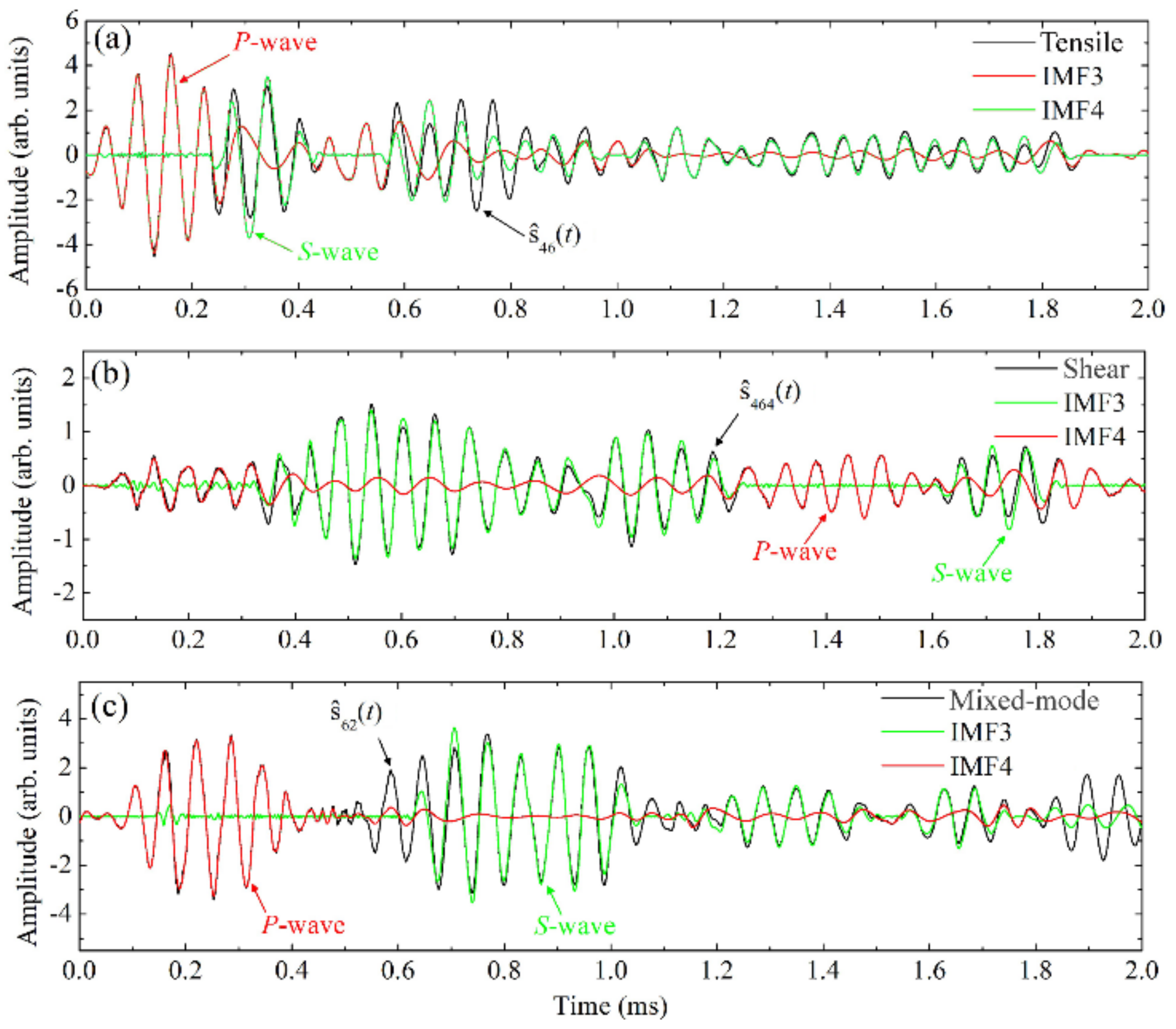
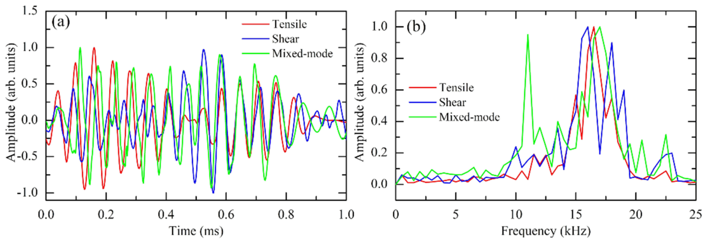
3.1. Characterization of Different Crack Events

It is well known that the waveform of an AE signal is intrinsically representative of the nature of the underlying fracture modes, which generate tensile, shear or mixed-mode deformations. Therefore, the timely characterization of these cracking events can act as a safe measure against the final collapse [6]. As demonstrated in [46], we rely upon the versatility of HHT to analyze AE signals for denoising as well as extracting their intrinsic mode functions (IMFs). Due to the IMFs, we can highlight the main characteristics of such different types of solicitations. In Figure 3a–c, we illustrate a comparison among tensile, shear and mixed-mode events ${\widehat{s}}_q\left(t\right)$ by focusing on their distinctive IMF components.

Figure 3a represents an AE time trace as emitted during a tensile event (Mode I). When a tensile event takes place, the moving sides of the crack lead to a transient volumetric change in the material. Consequently, most of the energy is released in the form of P-waves, which are faster [60], whereas only a limited amount is transferred into S-waves, which are slower. We use HHT to extract the relevant components of the solicitation. As expected, the AE wave (black line) is constituted by a large P-wave (IMF3, red line) [61], followed by a S-wave (IMF 4, green line) having a smaller amplitude [62]. For tensile events, the RT is short [63], and then a high RA is observed.

Figure 3b displays an AE time trace as emitted during a shear event (Mode II). In this case, the shape (and not the volume) of the material changes once in proximity of the crack. On this occasion, the shear crack (black line) emits most of the energy in the form of S-waves (IMF3, green line) and only a small amount in the form of P-waves (IMF4, red line). In terms of AE parameters, this cracking event is described by a long RT and a short RA [18].

Figure 3c displays an example of time trace for a mixed mode (Mode III) which is typically observed during the transition from a tensile dominant regime to a shear dominant one. Mixed modes are originated from a combination of tensile and shear cracks [64,65,66] and are important for a wide range of civil engineering [13,66,67,68]. Such events can be described by a balanced combination of P-wave (IMF3, green line) and S-waves (IMF4, red line) [64]. Nonetheless, the mixed-modes cannot be properly identified by calculating AE parameters, such as RT or RA [10]. Therefore, a more flexible approach is required to discriminate among different classes of failures. The proposed classification of the main fracture modes is based on the approach as described in [46] and confirmed in [69,70,71,72]. Our experimental measurements show AE data as characterized by the generation of tensile, shear as well as mixed-mode events.

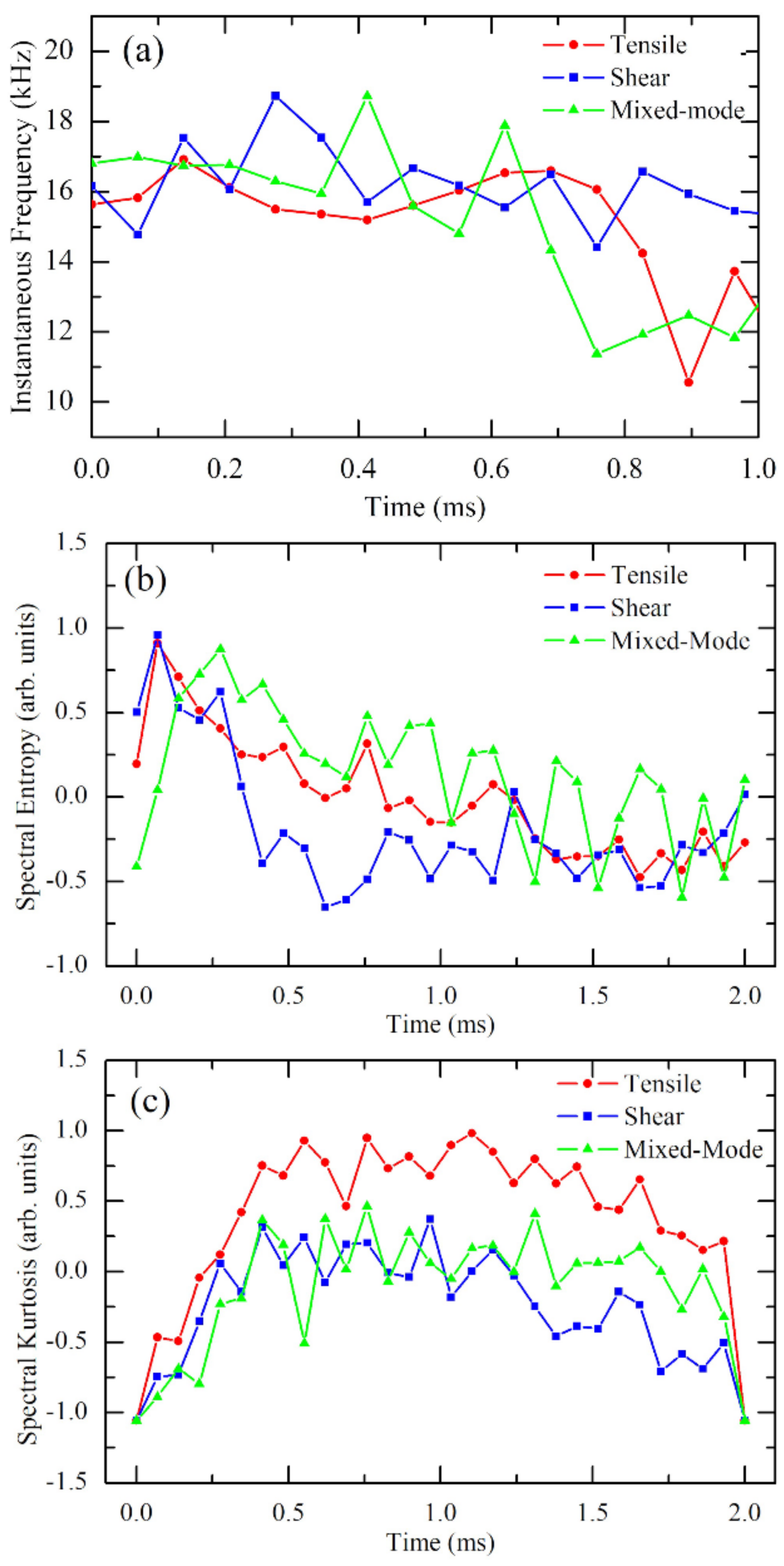
3.2. Analysis of Acoustic Emission Events Using Feature Extraction

In order to envisage both realistic and large-scale applications, the classification process must be as fast and reliable as possible. Thus, each AE preprocessed waveform, ${\widehat{s}}_q\left(t\right)$, is turned into a compact representation through a set of Γ_q features, in both time and frequency domains. Figure 4a shows an example of time domain traces of three different reference signals ${\widehat{s}}_q\left(t\right)$ from tensile (red line), shear (blue line) and mixed-mode events (green line), and their Fourier spectra (Figure 4b), respectively. We have used both time and frequency information to calculate the instantaneous frequency, spectral entropy and spectral kurtosis as summarized in Table 1. For the sake of consistency, we will also generally refer later to these properties as event descriptors (EDs).

3.2.1. Instantaneous Frequency

The IF of a nonstationary signal is a time-varying parameter that relates to the average frequencies of the signal [77,78] and it is computed as the derivative of the phase of the analytic signal of the input [59]. In order to extract it, we have performed the following calculations:

• Compute first the analytic signal $z\left(t\right)$ of the input, $s\left(t\right)$, such that $z\left(t\right)=s\left(t\right)+jH\left\{s\left(t\right)\right\}=A\left(t\right)e^{j\varphi \left(t\right)}$, where $H\left(t\right)$ is the Hilbert Transform of $s\left(t\right)$, $A\left(t\right)$ is defined as the instantaneous power, whereas $\varphi \left(t\right)$ is the instantaneous phase;
• Estimate the instantaneous frequency from the following time derivative:

  $$IF\left(t\right)=\frac{1}{2\pi }\frac{d\varphi }{dt}$$

  (3)

A plot of IF as calculated from the signals of Figure 4a is shown in Figure 5a. Those data extend the information of the Fourier spectra showing the range of time where the modes are excited.

3.2.2. Spectral Entropy

The SE [30] of a signal is a measure of its spectral power distribution. The SE treats the signal normalized power distribution in the frequency domain as a probability distribution and calculates the Shannon entropy of it. The Shannon entropy, in the AE context, is the spectral entropy of the signal s(t). This property has already shown to be useful for features extraction in fault detection and diagnosis [79]. The equations for SE arise from the equations for the power spectrum and probability distribution for a signal.

If the domain of definition for s(t) is restricted to a set of discrete points t_n = nT, where n is an integer and T is the sampling period, the signal s(t_n) is called a discrete-time signal. For such discrete time-varying signal s(t_n), the frequency power spectrum (PS) can be defined as $PS\left(f\right)={\left|S\left(f\right)\right|}^2$, where $S\left(f\right)$ is the discrete Fourier transform of s(t_n). The probability distribution function $PDF\left(f\right)$ is then written as:

$$PDF\left(f\right)=\frac{PS\left(f\right)}{{\displaystyle \sum _{i}PS\left(i\right)}}$$

(4)

The normalized spectral entropy $SE$ is a function of frequency and follows as:

$$SE\left(f\right)=-\frac{{\displaystyle \sum _{m=1}^{M}PDF\left(m\right){\log }_2\left(PDF\left(m\right)\right)}}{{\log }_{2}M}$$

(5)

where M is the total number of frequency points derived by the Fourier transform and equal to half the length of the time series x(t_n). The denominator ${\log }_{2}M$ represents the maximal value for the spectral entropy of white noise, which is uniformly distributed in the frequency domain. A plot of SE as calculated from the different signals of Figure 4a is shown in Figure 5b. As illustrated, peculiar differences can be observed from the SE of the signals. These differences will contribute to DL-based classification, although they are not easily classifiable by humans. However, from the viewpoint of power distribution among different frequency components, there is a relationship between IF and SE. We have noticed a substantial agreement with the mechanics of the events, which precedes the transition from a prevalent damage process to the other one. Such transitory coexistence is well represented by the corresponding decrease in SE, which evidences a distinctive pattern in mixed-mode deformations when compared to tensile and shear damages. [10,13,64,66,80].

3.2.3. Spectral Kurtosis

The SK [31,76] is a statistical tool that can identify the non-Gaussian behavior in the frequency domain. SK has been effectively used for detecting and extracting signals associated with faults in rotating mechanical systems [81]. The SK, or $\kappa \left(f\right)$, of a time-varying input signal s(t) can be computed based on the short-time Fourier transform (STFT) of the signal, S(t,f):

$$SK\equiv \kappa \left(f\right)=\frac{〈{\left|S\left(t,f\right)\right|}^4〉}{〈{\left|S\left(t,f\right)\right|}^2〉}-2=\frac{m_4\left\{\left|z\left(t\right)\right|\right\}}{{\left(m_2\left\{\left|z\left(t\right)\right|\right\}\right)}^2}-2$$

(6)

where $f\ne 0$ and $〈\dots 〉$ is the time-average operator, whereas $m_4$ and $m_2$ are the raw 4th and 2nd order moments, respectively [31]. Figure 5c shows the SK as calculated from the signals of Figure 4a. The SK for tensile events (red line) is positive and higher than the corresponding function for shear (blue line) and mixed-mode (green line) events. Particularly, any SK point falling within 5–22 kHz (mostly above SK = 1.0) is likely to be non-stationary and non-Gaussian [82]. A possible explanation is that tensile modes are characterized by a large generation of (short-lived) micro-displacements associated with the opposite movements of the crack surfaces [83] whose spectral components do not exhibit a normal distribution. The occurrence of several transient events causes multiple discontinuities in the analyzed signal, which are well-captured by SK whereas other operators (for instance, power spectral density) are not able to preserve such information [31].

Indeed, it is reasonable to assume that high frequency components are generated by such small discontinuities, that mainly distinguish the tensile [84,85] from shear fracture, whereas relevant frequency contributions are the results of few but larger deformations that usually develop during the final collapse [16]. It is well-known how variations in the shape of the waveform during the loading process identify a change in the dominant damage mechanism of the specimen. Shear events and mixed-mode events are characterized by smaller values of SK if compared to tensile deformations. This is because a shear event generates a relatively smaller number of transients, which corresponds to a lower value of SK, (here is slightly above 0). Interestingly, we observe that mixed-modes exhibit predominantly the lowest SK (between 5 to 20 kHz) and in particular around 11 kHz the SK = −0.5 which represents a locally stationary behavior. This is because the signal maintains a relatively constant amplitude at the corresponding frequency (as shown in Figure 5c).

3.3. Deep Learning and Bidirectional Long-Short Time Memory

The DL represents a relatively recent branch of machine learning research [34], which attempts to model hierarchical representations behind data and classify or predict patterns by combining multiple features [10,11,12,13]. A DL network is composed of several layers, each representing a function able to apply a transformation from the input to the output. Such layers are stacked together according to the main scope (i.e., classification, prediction, recognition) and are characterized by independent properties and parameters, that affect the way they contribute to the final objective. In addition, other variables of the DL structure (i.e., number of layers, input size and characteristics, number of elements used for the training and validation purposes) are able to impact on its performance, for which we commonly refer to as model-parameters. Here, we propose a DL-based model with the aim to identify the AE among different classes of crack events. We use the Bi-LSTM network which is a promising solution for the problem of time series identification [86]. Considering the theoretical fundamentals of RNNs, in a standard LSTM cell [38], the response (output) to a given input $x\left(t\right)$, at time t, is determined by the interplay of various elements, called gates, which have different behaviors. Among them, the “forget gate” $f\left(t\right)$ controls which information should be forgotten from the previous cell hidden state, h(t − 1). The output gate $y\left(t\right)$ highlights which information should be going to the next hidden state $h\left(t\right)$. The flow diagram is shown in Figure 6 where an unfolded structure for a sequence of three consecutive steps (t − 1, t, t + 1) is provided.

At each time step t, the hidden state h(t) is updated by a combination of: (1) current data of the input vector at the same time step, $x\left(t\right)$, (2) the hidden state at the previous time-step h(t − 1), (3) the input gate i(t), (4) the forget gate f(t), (5) the output gate o(t), (6) the weight matrix $W$, (7) and a memory cell c(t). Specifically, $W_i$, $W_f$, $W_o$ and $W_c$ are the weight matrices mapping the hidden layer input h(t) to the three gates i(t), f(t), o(t) and the input cell state c(t), while $V_i$, $V_f$, $V_o$ and $V_c$ are the weight matrices connecting the previous cell output state y(t − 1) to the three gates and the input cell state. On the other hand, $b_f$, $b_i$, $b_o$, $b_c$ are the bias vectors of LSTM cell during training, which are regarded as parameters of the input, forget, output gates and cell state c(t) respectively.

This such architecture, the Bi-LSTM is able to process the input sequence in both directions (forward and backward) with two separate hidden layers in order to account for the full input context. The following equations define the corresponding hidden layer function, whereas the $\to$ and $\leftarrow$ denote the forward and backward process, respectively. We can express the forward $\to$ direction of the process such as:

$$\begin{array}{l}\overrightarrow{i}\left(t\right)=\alpha \left({\overrightarrow{W}}_i\overrightarrow{x}\left(t\right)+{\overrightarrow{V}}_i\overrightarrow{h}\left(t-1\right)+{\overrightarrow{b}}_i\right)\\ \overrightarrow{f}\left(t\right)=\alpha \left({\overrightarrow{W}}_f\overrightarrow{x}\left(t\right)+{\overrightarrow{V}}_f\overrightarrow{h}\left(t-1\right)+{\overrightarrow{b}}_f\right)\\ \overrightarrow{o}\left(t\right)=\alpha \left({\overrightarrow{W}}_o\overrightarrow{x}\left(t\right)+{\overrightarrow{V}}_o\overrightarrow{h}\left(t-1\right)+{\overrightarrow{b}}_o\right)\\ \overrightarrow{c}\left(t\right)=\left[\overrightarrow{f}\left(t\right)\odot \overrightarrow{c}\left(t-1\right)\right]+\left[\overrightarrow{i}\left(t\right)\odot \tanh \left({\overrightarrow{W}}_c\overrightarrow{x}\left(t\right)+{\overrightarrow{V}}_c\overrightarrow{h}\left(t-1\right)+{\overrightarrow{b}}_c\right)\right]\\ \overrightarrow{h}\left(t\right)=\overrightarrow{o}\left(t\right)\odot \tanh \left(\overrightarrow{c}\left(t\right)\right)\end{array}$$

(7)

where α is the activation function which normally is represented by the sigmoid function, the tanh is the hyperbolic tangent function, and $\odot$ is the element-wise product. We can express the formulas for the backward process using the same formula:

$$\begin{array}{l}\overleftarrow{i}\left(t\right)=\alpha \left({\overleftarrow{W}}_i\overleftarrow{x}\left(t\right)+{\overleftarrow{V}}_i\overleftarrow{h}\left(t+1\right)+{\overleftarrow{b}}_i\right)\\ \overleftarrow{f}\left(t\right)=\alpha \left({\overleftarrow{W}}_f\overleftarrow{x}\left(t\right)+{\overleftarrow{V}}_f\overleftarrow{h}\left(t+1\right)+{\overleftarrow{b}}_f\right)\\ \overleftarrow{o}\left(t\right)=\alpha \left({\overleftarrow{W}}_o\overleftarrow{x}\left(t\right)+{\overleftarrow{V}}_o\overleftarrow{h}\left(t+1\right)+{\overleftarrow{b}}_o\right)\\ \overleftarrow{c}\left(t\right)=\left[\overleftarrow{f}\left(t\right)\odot \overleftarrow{c}\left(t+1\right)\right]+\left[\overleftarrow{i}\left(t\right)\odot \tanh \left({\overleftarrow{W}}_c\overleftarrow{x}\left(t\right)+{\overleftarrow{V}}_c\overleftarrow{h}\left(t+1\right)+{\overleftarrow{b}}_c\right)\right]\\ \overleftarrow{h}\left(t\right)=\overleftarrow{o}\left(t\right)\odot \tanh \left(\overleftarrow{c}\left(t\right)\right)\end{array}$$

(8)

Then, the complete Bi-LSTM hidden element representation h(t) is the concatenated vector of the outputs from both forward (Equation (7)) and backward (Equation (8)) processes, such that:

$$h\left(t\right)=\overrightarrow{h}\left(t\right)\oplus \overleftarrow{h}\left(t\right)$$

(9)

Here, the two sub-layers compute forward $\overrightarrow{h}\left(t\right)$ and backward $\overleftarrow{h}\left(t\right)$ hidden sequences, respectively, which are then combined to generate the output sequence $y\left(t\right)$ as the concatenation of both input sequences, $y\left(t\right)=h\left(t\right)x\left(t\right)$. Bi-LSTM units are a key element in our DL model because of their ability to classify, process and predict time series with time lags of unknown duration. Relative insensitivity to gap length gives an advantage to Bi-LSTMs over alternative RNNs, hidden Markov models and other sequence learning methods [87].

3.4. DL-Based Event-Type Discrimination

Diverse concrete types (e.g., fiber reinforced concrete, pre-stressed concrete) are used in the literature for investigating failure mechanisms using AE signals. An acoustic wave comprises of characteristic sub-events, which can be categorized into a few main classes, where the shape of waveform is directly connected to the type of deformation, as also explained in Section 3.1.

To determine the crack type, various statistical properties of the signal have been considered (see Section 3.2). Thus, we use a combination of these properties to feed a DL network able to distinguish among such different classes of events.

The internal structure of block (III.2) is shown in Figure 7. Here, the DL model is organized by means of the interposition of functional layers aimed at providing convergence of training and regularization methodology. In this way, a trained mode is able to find solutions with predictable performance. Generalization to data outside the training set is the key objective of predictive machine learning methods. In this block, the input features array, Γ, is used to train the DL network and identify different crack events. We use Bi-LSTM units as a key ingredient for this classification problem. In our scenario, the classes of events are categorized into [13]:

• Tensile event [10,88,89];
• Shear event [13,90,91,92];
• Mixed mode [64,67,68,93,94,95,96].

Once the input training data Γ are collected at the bottom of the network (first block on the left), they are used to feed a stack composed of several layers. Firstly, we have a cascade of different Bi-LSTM layers constituted by N₁ and N₂ hidden units, respectively. The output of the first Bi-LSTM layer is then used as input for the subsequent activation function layer, which is represented by a rectified linear unit (ReLU) [97]. ReLU has been demonstrated to be particularly valuable for the study of the classification or prediction once applied on time sequences and has been shown to outperform more conventional approaches based on previous sigmoid and tanh functions [98].

In our DL model, each element of the output of ReLU layer flows through a second Bi-LSTM block having N₂ cells, then a fully-connected layer is interposed. It multiplies the input by a weight matrix and then adds a bias vector. The default for the initial weights is a Gaussian distribution with mean zero and unit variance, whereas the initial value for the bias is 0. Given the nature of the classification task, a subsequent Softmax layer [99] constitutes an essential part at the top of the DL network. Here, the Softmax function y_j is applied to the input x using the following expression:

$$y_j\left(x\right)=\frac{\exp \left(a_j\left(x\right)\right)}{{\displaystyle \sum _{k=1}^K\exp \left(a_k\left(x\right)\right)}}, \mathrm{where} 0\le y_j\le 1 \mathrm{and} {\displaystyle \sum _{k=1}^K{y}_k=1}$$

(10)

where $P\left(c_j|x,\theta \right)$ represents the conditional probability of the sample given the class $j$ (j = 1, 2, … K, $j\ne k$) among K classes, with $P\left(c_j\right)$ being the class prior probability. If we set $y_j\left(x\right)=P\left(c_j|x,\theta \right)$ and define $a_j=\ln \left(P\left(x,\theta |c_j\right)P\left(c_j\right)\right)$, we obtain from Equation (10) [100]:

$$y_j\left(x\right)=P\left(c_j|x,\theta \right)=\frac{P\left(x,\theta |c_j\right)P\left(c_j\right)}{{\displaystyle \sum _{k=1}^{K}P\left(x,\theta |c_k\right)P\left(c_k\right)}}$$

(11)

Specifically, the predicted probability for the class j given a sample vector x and a weighting vector θ, such that $0\le P\left(c_j|x,\theta \right)\le 1$ and ${\displaystyle \sum _{k=1}^{K}P\left(c_k|x,\theta \right)=1}$.

Finally, a classification layer [99] is the last (top of the DL network) and it computes the cross entropy (CE) loss [98]. This loss function $J$ depends in general on the parameters matrix ${\Theta }$ which accounts for the weights of the defined model. For multiclass classification problems with mutually exclusive classes, we can write the CE as [99]:

$$J\left({\Theta }\right)=-\frac{1}{Q}{\displaystyle \sum _{q=1}^Q{\displaystyle \sum _{k=1}^K{w}_k{t}_{qk}\ln \left(y_{qk}\right)}}$$

(12)

where Q is the number of samples, K is the number of classes, $w_k$ is the weight for class k (k = 1,2, … K), $t_{qk}$ is the indicator that the q-th sample belongs to the k-th class, and $y_{qk}$ is the output for sample q for class k, which in this case, is the value from the Softmax function (corresponding the probability that the network associates the q-th input with class k).

Therefore, the output of the top layer is the most probable class according to the way the DL-network has been trained.

3.4.1. Training Model

Although the proposed Bi-LSTM network is composed of several layers L, it can still abstracted as a function $F$ of input x with a parameters matrix Θ:

$$\left[\widehat{y}\right]=F\left(x,\mathsf{\Theta }\right)$$

(13)

where $\widehat{y}$ is the estimated output, and Θ represents all the weights w_i and biases γ_i for all the layers $\left(i=1,\dots L\right)$:

$$\mathsf{\Theta }={\left[w_i,{\gamma }_i\right]}_{i=1,\dots L}$$

(14)

By using the mini-batch stochastic gradient descent method (SGDM) [98], Θ can be optimized to minimize the CE, having chosen CE as loss function $J$. By applying the training algorithm back-propagation through time (BPTT) [14], the following numerical computation is iteratively performed to update the parameters to lower the loss function $J$ toward the optimum:

$$\overline{\mathsf{\Theta }}=\mathsf{\Theta }-r_l\frac{\partial J\left(\mathsf{\Theta }\right)}{\partial \mathsf{\Theta }}$$

(15)

where we use gradient descent to adjust the learning rate $r_l$ automatically. Early stopping is also applied to prevent overfitting [16]. Data samples are prepared in advance for the training process. The construction and the training process of the model are both implemented using the latest TensorFlow [101]. Totally 15,000 digitized samples are gathered for the training of the BiLSTM model and 1650 are used for testing purposes, both come with equally balanced classes obtained via data augmentation.

3.4.2. Model-Parameter Settings

There are multiple model-parameters in our proposed method that have an effect on the performance: (1) the size of the training dataset $Q$, (2) the combination different EDs which affects the size of the input array Γ_q, (3) the total number d_LSTM = N₁ + N₂ of memory cells in the model, which affects the complexity of the network, and (4) the number of epochs Ɛ used to train the network. As stated above, being that the size of $Q$ is considered suitable for the training, we have to find the optimal value for ${\lambda }_r$, d_LSTM and Ɛ in order to achieve the most accurate classification of crack events.

4. Results and Discussions

An extensive preliminary study has been carried out to identify, collect and categorize tensile, shear and mixed-modes as the recognized classes of deformation. The results we have achieved in processing the AE data are qualitatively similar for all the specimens tested. Thus, we discuss in detail the results from one dataset, which represents an ensemble of crack events from multiple specimens. Only part of such measurements has been improved via data augmentation [102,103] to ensure the required balance between the different types of failure. For a given event ${\widehat{s}}_q\left(t\right)$ in any class (i.e., tensile, shear and mixed-mode), an array of Q rows and proportional to the number of EDs is calculated and used to populate the training dataset. Each ED is then represented by a series composed of N_ED elements. Such input dataset is therefore constituted of Q-x-(number of EDs)-x-N_ED, whose details are provided in

Table 2. Description of the components of each combination of inputs λ₁–λ₅ used to train the DL-network.

Available Inputs	Signal	IF	SE	SK	Size of Input DATASET Γq
λ1	yes	no	no	no	Q × 1 × NED
λ2	no	yes	no	no	Q × 1 × NED
λ3	no	yes	yes	no	Q × 2 × NED
λ4	no	yes	no	yes	Q × 2 × NED
λ5	no	yes	yes	yes	Q × 3 × NED

. Standardization is applied on the data to ensure zero mean and unit variance and to ease the training process. In order to avoid over-fitting during the learning process and improve classification accuracy, the dataset was divided into training and validation quotas with an 80/20 ratio.

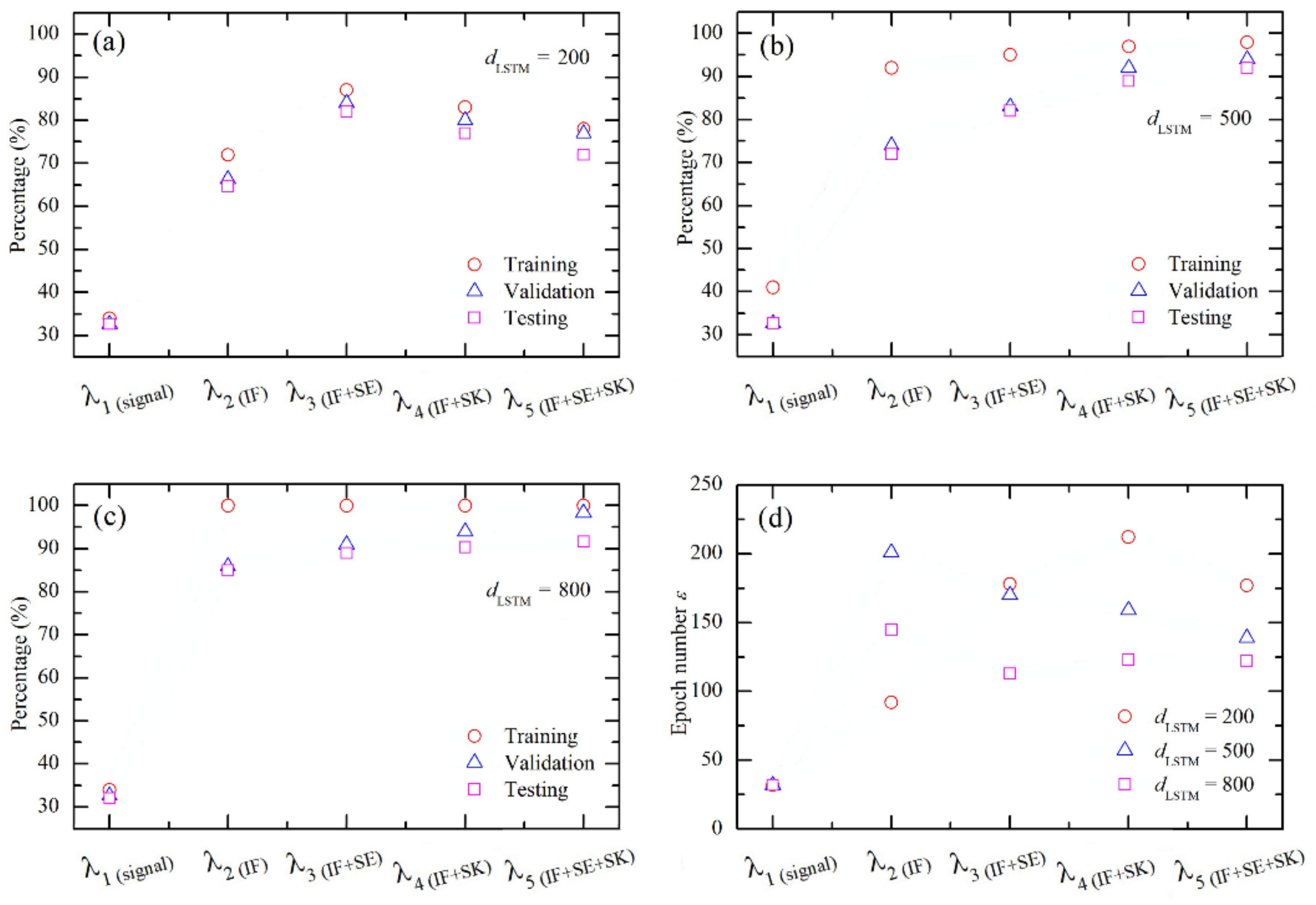
Performance Optimization of Model-Parameters

We have used a training dataset containing Q = 15,000, mini-batch sample size $m$ = 1500, N_ED = 67, initial learning rate $r_l=0.001$ using SGDM optimizer. We evaluated a different number of hidden units of the network d_LSTM = 200, 500 and 800, for various configurations of EDs as input data λ₁–λ₅ (see Table 2). For all the applications, we considered a maximum number of epochs Ɛ = 220, to avoid overfitting the learning process stops when the loss function does not decrease after 30 epochs [98]. We conducted several numerical tests to determine the optimal configuration.

Figure 8a–c summarizes the effect of the number of d_LSTM (or hidden units) on classification accuracy (i.e., ratio between the number of correctly classified events and the total number of events in the considered dataset, in percentage) for the training, validation and test dataset (testing) of the proposed model (d_LSTM = 200 in Figure 8a, d_LSTM = 500 in Figure 8b, and d_LSTM = 800 in Figure 8c). Here, we can observe that the performance of this model is better as the number d_LSTM increases under the defined range (d_LSTM = [200–800]), while it does not undergo saturation or degradation as the scale becomes larger. A value of d_LSTM = 500 provides the best testing performance with an accuracy of 92% (by combining IF, SE and SK). The reason is that the Bi-LSTM model with fewer LSTM cells suffers from lack of capability of long-term memory, which will result in under-fitting, whereas a model too large (i.e., higher number of hidden cells) will always lead to increasing difficulty due to over-fitting. In Figure 8d, we show the validation performance of Bi-LSTM models in terms of epochs (required to complete the training) for different numbers of cells and inputs (λ₁–λ₅). After the training is completed, the model has learned the patterns necessary for the classification of the input events. As expected, the epoch number Ɛ of each model is different, depending on the choice of d_LSTM, and the input configuration λ_r. We also observed that varying λ_r does not significantly impact on the computing time. This is because the training job is mainly affected by both the size Q of the training dataset, and the complexity of the network d_LSTM during weights updating and gradient propagation. We only adopted the parameter matrix Θ that generates the lowest J(Θ) on the input dataset and collected the value of J for both training, J_TRN(Θ), and validation J_VAL(Θ). The training, validation and testing accuracies increase with λ_r when d_LSTM is higher than 200 LSTM cells. For d_LSTM = 200, a local minimum in validation loss is observed with λ_r = λ₃ (which implies using a combination of IF and SE for each acoustic signal). Epoch number Ɛ tends to decrease with d_LSTM. As expected, the Ɛ required for the calculation of the three different statistical measures λ₅ (which implies using IF, SE and SK for each signal) is the lowest.

Figure 9 provides the confusion matrix, which details the testing performance for d_LSTM = 500 and by considering the combination of IF, SE and SK as input (λ₅). Overall, the accuracy as calculated on the testing dataset (1650 samples of equally balanced classes) accounts for 92%. As it can be observed, the better intra-class accuracy is achieved by classifying shear events (93.1%), followed by tensile event (91.9%), where the lowest is mixed-mode (90.0%). The model finds most difficult to identify mixed-modes and mainly confuses them with actual tensile solicitations (or vice versa). On the other hand, the shear events appear to be relatively easier to be classified when compared against the other classes, with a limited number of false positives mainly concentrated on mixed-modes.

Figure 10 shows the learning error by the value of the loss function for both training (Figure 10a) and validation (Figure 10b) tasks.

Based on these analyses, we set the number of the LSTM cells in our Bi-LSTM model to d_LSTM = 500, since it provides the lowest validation loss (J_VAL(Θ)) and the better testing accuracy (according to Figure 8c), and choose the input configuration λ₅ where we take into account IF, SE and SK as the representative properties of the signal.

5. Conclusions

In summary, this work describes the strategy to develop a deep neural network with Bi-LSTM for the classification of time domain AE signals. The key ingredient is a proper selection of EDs we found to be the instantaneous frequency, spectral entropy and spectral kurtosis. These EDs have proven to reflect distinctive properties of the cracks’ events. In particular, our results show that the use of such EDs as the input of a DL-based network gives rise to an overall accuracy of 92%. This promising perspective stimulates further innovative research scenarios aimed at devising new EDs and novel interpretative approaches to better categorize acoustic events and to correlate their occurrence with the damage mechanisms that take place during the cracking phenomenon. We wish to highlight that this approach has been implemented for fault diagnosis/classification problems in concrete structures, but it can be generalized for the characterization of damages in other materials, such as rubberized concrete [104], or for predicting failures with minimum adjustments and moderate re-training [98]. In addition, the methods presented here provide capabilities for real time monitoring in large scale applications and might be suitable to be implemented in the sensing layer [105,106] of future IoT-based monitoring systems [107] as well as for digital twin applications in the construction industry [108].

References

1. Farrar, C.R.; Worden, K. An introduction to structural health monitoring. Philos. Trans. R. Soc. A Math. Phys. Eng. Sci. 2007, 365, 303–315. [Google Scholar] [CrossRef] [PubMed]
2. Aggelis, D.G. Classification of cracking mode in concrete by acoustic emission parameters. Mech. Res. Commun. 2011, 38, 153–157. [Google Scholar] [CrossRef]
3. Carpinteri, A.; Lacidogna, G.; Niccolini, G.; Puzzi, S. Critical defect size distributions in concrete structures detected by the acoustic emission technique. Meccanica 2007, 43, 349–363. [Google Scholar] [CrossRef]
4. Carpinteri, A.; Lacidogna, G.; Accornero, F.; Mpalaskas, A.C.; Matikas, T.E.; Aggelis, D.G. Influence of damage in the acoustic emission parameters. Cem. Concr. Compos. 2013, 44, 9–16. [Google Scholar] [CrossRef]
5. Chai, M.; Zhang, Z.; Duan, Q. A new qualitative acoustic emission parameter based on Shannon’s entropy for damage monitoring. Mech. Syst. Signal Process. 2018, 100, 617–629. [Google Scholar] [CrossRef]
6. Aggelis, D.; Shiotani, T.; Papacharalampopoulos, A.; Polyzos, D. The influence of propagation path on elastic waves as measured by acoustic emission parameters. Struct. Health Monit. 2012, 11, 359–366. [Google Scholar] [CrossRef]
7. Lamonaca, F.; Sciammarella, P.; Scuro, C.; Carni, D.; Olivito, R. Internet of things for structural health monitoring. In Proceedings of the 2018 Workshop on Metrology for Industry 4.0 and IoT, Brescia, Italy, 16–18 April 2018; pp. 95–100. [Google Scholar]
8. Colombo, S.; Forde, M.; Main, I.; Shigeishi, M. Predicting the ultimate bending capacity of concrete beams from the “relaxation ratio” analysis of AE signals. Constr. Build. Mater. 2005, 19, 746–754. [Google Scholar] [CrossRef]
9. Proverbio, E. Evaluation of deterioration in reinforced concrete structures by AE technique. Mater. Corros. 2010, 62, 161–169. [Google Scholar] [CrossRef]
10. Grosse, C.U.; Ohtsu, M. (Eds.) Acoustic Emission Testing; Springer: Berlin/Heidelberg, Germany, 2008; ISBN 978-3-540-69895-1. [Google Scholar]
11. Carnì, D.L.; Scuro, C.; Lamonaca, F.; Olivito, R.S.; Grimaldi, D. Damage analysis of concrete structures by means of b-value technique. Int. J. Comput. 2017, 16, 82–88. [Google Scholar] [CrossRef]
12. Moment Tensor Analysis of Acoustic Emission for Cracking Mechanisms in Concrete. ACI Struct. J. 1998, 95, 87–95. [CrossRef]
13. Ohno, K.; Ohtsu, M. Crack classification in concrete based on acoustic emission. Constr. Build. Mater. 2010, 24, 2339–2346. [Google Scholar] [CrossRef]
14. Aggelis, D.; Mpalaskas, A.; Matikas, T. Investigation of different fracture modes in cement-based materials by acoustic emission. Cem. Concr. Res. 2013, 48, 1–8. [Google Scholar] [CrossRef]
15. Shahidan, S.; Pulin, R.; Bunnori, N.M.; Holford, K. Damage classification in reinforced concrete beam by acoustic emission signal analysis. Constr. Build. Mater. 2013, 45, 78–86. [Google Scholar] [CrossRef] [Green Version]
16. Ohtsu, M.; Shigeishi, M.; Iwase, H.; Koyanagit, W. Determination of crack location, type and orientation in a concrete structures by acoustic emission. Mag. Concr. Res. 1991, 43, 127–134. [Google Scholar] [CrossRef]
17. Shahidan, S.; Pullin, R.; Holford, K.M.; Bunnori, N.M.; Noor, N.M. Quantitative evaluation of the relationship between tensile crack and shear movement in concrete beams. Adv. Mater. Res. 2012, 626, 355–359. [Google Scholar] [CrossRef] [Green Version]
18. Aggelis, D.; Mpalaskas, A.; Ntalakas, D.; Matikas, T. Effect of wave distortion on acoustic emission characterization of cementitious materials. Constr. Build. Mater. 2012, 35, 183–190. [Google Scholar] [CrossRef]
19. Mpalaskas, A.; Thanasia, O.; Matikas, T.; Aggelis, D. Mechanical and fracture behavior of cement-based materials characterized by combined elastic wave approaches. Constr. Build. Mater. 2014, 50, 649–656. [Google Scholar] [CrossRef]
20. Bungey, J.H.; Grantham, M.G. Testing of Concrete Structures; CRC Press: Boca Raton, FL, USA, 2006; ISBN 9780415263016. [Google Scholar]
21. Morizet, N.; Godin, N.; Tang, J.; Maillet, E.; Fregonese, M.; Normand, B. Classification of acoustic emission signals using wavelets and Random Forests: Application to localized corrosion. Mech. Syst. Signal Process. 2016, 70–71, 1026–1037. [Google Scholar] [CrossRef]
22. Zhang, M.; Li, J.; Xu, J.; Zheng, J.; Zhang, Q. Wood Acoustic Emission Signals Classification Based on Pseudospectrum, and Entropy. J. Phys. Conf. Ser. 2021, 2005, 012048. [Google Scholar]
23. Deshpande, P.; Pandiyan, V.; Meylan, B.; Wasmer, K. Acoustic emission and machine learning based classification of wear generated using a pin-on-disc tribometer equipped with a digital holographic microscope. Wear 2021, 476, 203622. [Google Scholar] [CrossRef]
24. Nasiri, S.; Khosravani, M.R. Machine learning in predicting mechanical behavior of additively manufactured parts. J. Mater. Res. Technol. 2021, 14, 1137–1153. [Google Scholar] [CrossRef]
25. Kim, K.B.; Kang, H.Y.; Yoon, D.J.; Choi, M.Y. Pattern classification of acoustic emission signals during wood drying by principal component analysis and artificial neural network. Key Eng. Mater. 2005, 297–300, 1962–1967. [Google Scholar] [CrossRef]
26. Li, J.; Du, G.; Jiang, C.; Jin, S. The classification of acoustic emission signals of 304 stainless steel during stress corrosion process based on K-means clustering. Anti Corros. Methods Mater. 2012, 59, 76–80. [Google Scholar] [CrossRef]
27. Barat, V.; Kostenko, P.; Bardakov, V.; Terentyev, D. Acoustic signals recognition by convolutional neural network. Int. J. Appl. Eng. Res. 2017, 12, 3461–3469. [Google Scholar]
28. Wu, J.-D.; Wong, Y.-H.; Luo, W.-J.; Yao, K.-C. Acoustic emission signal classification using feature analysis and deep learning neural network. Fluct. Noise Lett. 2020, 20, 2150030. [Google Scholar] [CrossRef]
29. Xin, H.; Cheng, L.; Diender, R.; Veljkovic, M. Fracture acoustic emission signals identification of stay cables in bridge engineering application using deep transfer learning and wavelet analysis. Adv. Bridge Eng. 2020, 1, 6. [Google Scholar] [CrossRef]
30. Pan, Y.N.; Chen, J.; Li, X.L. Spectral entropy: A complementary index for rolling element bearing performance degradation assessment. Proc. Inst. Mech. Eng. Part C J. Mech. Eng. Sci. 2009, 223, 1223–1231. [Google Scholar] [CrossRef]
31. Antoni, J. The spectral kurtosis: A useful tool for characterising non-stationary signals. Mech. Syst. Signal Process. 2006, 20, 282–307. [Google Scholar] [CrossRef]
32. Da Silva, W.R.L.; de Lucena, D.S. Concrete cracks detection based on deep learning image classification. In Proceedings of the 18th International Conference of experimental Mechanics (ICEM18), Brussels, Belgium, 1–5 July 2018; Volume 2, p. 489. [Google Scholar]
33. Jang, K.; Kim, N.; An, Y.-K. Deep learning–based autonomous concrete crack evaluation through hybrid image scanning. Struct. Health Monit. 2018, 18, 1722–1737. [Google Scholar] [CrossRef]
34. Goodfellow, I.; Bengio, Y.; Courville, A. Deep Learning; The MIT Press: Cambridge, MA, USA, 2016; ISBN 978-0-262-03561-3. [Google Scholar]
35. Wang, Z.; Yan, W.; Oates, T. Time series classification from scratch with deep neural networks: A strong baseline. In Proceedings of the 2017 International Joint Conference on Neural Networks (IJCNN), Anchorage, AK, USA, 14–19 May 2017; pp. 1578–1585. [Google Scholar]
36. Karim, F.; Majumdar, S.; Darabi, H.; Chen, S. LSTM Fully Convolutional Networks for Time Series Classification. IEEE Access 2018, 6, 1662–1669. [Google Scholar] [CrossRef]
37. Graves, A.; Schmidhuber, J. Framewise phoneme classification with bidirectional LSTM and other neural network architectures. Neural Netw. 2005, 18, 602–610. [Google Scholar] [CrossRef]
38. Hochreiter, S.; Schmidhuber, J. Long short-term memory. Neural Comput. 1997, 9, 1735–1780. [Google Scholar] [CrossRef] [PubMed]
39. Thireou, T.; Reczko, M. Bidirectional Long Short-Term Memory Networks for Predicting the Subcellular Localization of Eukaryotic Proteins. IEEE/ACM Trans. Comput. Biol. Bioinform. 2007, 4, 441–446. [Google Scholar] [CrossRef]
40. Mousa, A.E.-D.; Schuller, B. Deep bidirectional long short-term memory recurrent neural networks for grapheme-to-phoneme conversion utilizing complex many-to-many alignments. In Proceedings of the Annual Conference of the International Speech Communication Association, INTERSPEECH, San Francisco, CA, USA, 8–12 September 2016; pp. 2836–2840. [Google Scholar]
41. Yokoyama, S.; Matsumoto, T. Development of an automatic detector of cracks in concrete using machine learning. Procedia Eng. 2017, 171, 1250–1255. [Google Scholar] [CrossRef]
42. Shao, H.; Jiang, H.; Zhao, H.; Wang, F. A novel deep autoencoder feature learning method for rotating machinery fault diagnosis. Mech. Syst. Signal Process. 2017, 95, 187–204. [Google Scholar] [CrossRef]
43. Gan, M.; Wang, C.; Zhu, C. Construction of hierarchical diagnosis network based on deep learning and its application in the fault pattern recognition of rolling element bearings. Mech. Syst. Signal Process. 2016, 72–73, 92–104. [Google Scholar] [CrossRef]
44. Ohtsu, M.; Shiotani, T.; Shigeishi, M.; Kamada, T.; Yuyama, S.; Watanabe, T.; Suzuki, T.; van Mier, J.G.M.; Vogel, T.; Grosse, C.; et al. Recommendation of RILEM TC 212-ACD: Acoustic Emission and Related NDE Techniques for Crack Detection and Damage Evaluation in Concrete. Mater. Struct. 2010, 43, 1177–1181. [Google Scholar] [CrossRef] [Green Version]
45. Lamonaca, F.; Carrozzini, A. Sensors & Transducers of Acoustic Emissions in Civil Engineering Structures by Using Time Frequency. Representation 2010, 8, 42–53. [Google Scholar]
46. Siracusano, G.; Lamonaca, F.; Tomasello, R.; Garescì, F.; La Corte, A.; Carnì, D.L.; Carpentieri, M.; Grimaldi, D.; Finocchio, G. A framework for the damage evaluation of acoustic emission signals through Hilbert–Huang transform. Mech. Syst. Signal Process. 2016, 75, 109–122. [Google Scholar] [CrossRef]
47. Ohtsu, M.; Tomoda, Y. Phenomenological Model of Corrosion Process in Reinforced Concrete Identified by Acoustic Emission. ACI Mater. J. 2008, 105, 194–199. [Google Scholar] [CrossRef]
48. Mindess, S. Acoustic emission methods. In Handbook on Nondestructive Testing of Concrete Second Edition; CRC Press: Boca Raton, FL, USA, 2003; pp. 348–364. [Google Scholar]
49. Carpinteri, A.; Lacidogna, G.; Manuello, A. Localization accuracy of microcracks in damaged concrete structures. In Acoustic Emission and Critical Phenomena; CRC Press: Boca Raton, FL, USA, 2008; pp. 103–124. [Google Scholar]
50. Kaphle, M.; Tan, A. Study of Acoustic Emission Data Analysis Tools for Structural Health Monitoring Applications. Acoust. Emiss. 2010, 29, 243–250. [Google Scholar]
51. iTech Standards. UNI EN UNI EN 12390-3. Testing Hardened Concrete Part 3: Compressive Strength of Test Specimens. 2009. Available online: https://www.en-standard.eu/din-en-12390-3-testing-hardened-concrete-part-3-compressive-strength-of-test-specimens/ (accessed on 14 December 2021).
52. Wriggers, P.; Moftah, S. Mesoscale models for concrete: Homogenisation and damage behaviour. Finite Elem. Anal. Des. 2006, 42, 623–636. [Google Scholar] [CrossRef]
53. iTech Standards. UNI EN UNI EN 13477-2. Non-Destructive Testing-Acoustic Emission-Equipment Characteristic-Part 2: Verification of Operating Characteristic. 2011. Available online: https://www.en-standard.eu/une-en-13477-2-2011-non-destructive-testing-acoustic-emission-equipment-characterisation-part-2-verification-of-operating-characteristic/ (accessed on 14 December 2021).
54. Carpinteri, A.; Corrado, M.; Lacidogna, G. Heterogeneous materials in compression: Correlations between absorbed, released and acoustic emission energies. Eng. Fail. Anal. 2013, 33, 236–250. [Google Scholar] [CrossRef]
55. Garesci’, F. Static and dynamic analysis of bonded sandwich plates. Int. J. Adhes. Adhes. 2012, 33, 7–14. [Google Scholar] [CrossRef]
56. Shen, G.; Wu, Z.; Zhang, J. Advances in Acoustic Emission Technology: Proceedings of the World Conference on Acoustic Emission–2013; Springer: Berlin/Heidelberg, Germany, 2015; p. 158. [Google Scholar]
57. Munoz, D.; Lara, F.B.; Vargas, C.; Enriquez-Caldera, R. Position Location Techniques and Applications; Elsevier: Amsterdam, The Netherlands, 2009; ISBN 9780123743534. [Google Scholar]
58. Huang, N.E.; Shen, Z.; Long, S.R.; Wu, M.C.; Shih, H.H.; Zheng, Q.; Yen, N.-C.; Tung, C.C.; Liu, H.H. The empirical mode decomposition and the Hilbert spectrum for nonlinear and non-stationary time series analysis. Proc. R. Soc. A Math. Phys. Eng. Sci. 1998, 454, 903–995. [Google Scholar] [CrossRef]
59. Takahashi, H.; Oohara, K.-I.; Kaneyama, M.; Hiranuma, Y.; Camp, J.B. On Investigating Emd Parameters To Search for Gravitational Waves. Adv. Adapt. Data Anal. 2013, 05, 1350010. [Google Scholar] [CrossRef] [Green Version]
60. Köppel, S.; Grosse, C. Advanced acoustic emission techniques for failure analysis in concrete. In Proceedings of the World Conference on Non-Destructive Testing (WCNDT), Rome, Italy, 15–21 October 2000. [Google Scholar]
61. Aggelis, D.; Matikas, T. Effect of plate wave dispersion on the acoustic emission parameters in metals. Comput. Struct. 2012, 98–99, 17–22. [Google Scholar] [CrossRef]
62. Ono, K. Structural integrity evaluation by means of acoustic emission. In Acoustic Emission and Critical Phenomena; Jenny Stanford Publishing: Dubai, United Arab Emirates, 2008; Volume 25, pp. 13–27. [Google Scholar]
63. Soulioti, D.; Barkoula, N.; Paipetis, A.; Matikas, T.; Shiotani, T.; Aggelis, D. Acoustic emission behavior of steel fibre reinforced concrete under bending. Constr. Build. Mater. 2009, 23, 3532–3536. [Google Scholar] [CrossRef] [Green Version]
64. Carmona, J.R.; Ruiz, G.; del Viso, J.R. Mixed-mode crack propagation through reinforced concrete. Eng. Fract. Mech. 2007, 74, 2788–2809. [Google Scholar] [CrossRef]
65. Behnia, A.; Chai, H.; Yorikawa, M.; Momoki, S.; Terazawa, M.; Shiotani, T. Integrated non-destructive assessment of concrete structures under flexure by acoustic emission and travel time tomography. Constr. Build. Mater. 2014, 67, 202–215. [Google Scholar] [CrossRef]
66. Bocca, P.; Carpinteri, A.; Valente, S. Mixed mode fracture of concrete. Int. J. Solids Struct. 1991, 27, 1139–1153. [Google Scholar] [CrossRef]
67. Ohtsu, M.; Kaminaga, Y.; Munwam, M.C. Experimental and numerical crack analysis of mixed-mode failure in concrete by acoustic emission and boundary element method. Constr. Build. Mater. 1999, 13, 57–64. [Google Scholar] [CrossRef]
68. Qian, J.; Fatemi, A. Mixed mode fatigue crack growth: A literature survey. Eng. Fract. Mech. 1996, 55, 969–990. [Google Scholar] [CrossRef]
69. Chen, C.; Li, Y.; Axel, L.; Huang, J. Real time dynamic mri by exploiting spatial and temporal sparsity. Magn. Reson. Imaging 2015, 34, 473–482. [Google Scholar] [CrossRef]
70. Buj-Corral, I.; Álvarez-Flórez, J.; Domínguez-Fernández, A. Acoustic emission analysis for the detection of appropriate cutting operations in honing processes. Mech. Syst. Signal Process. 2018, 99, 873–885. [Google Scholar] [CrossRef]
71. Lin, L.; Chu, F. Feature extraction of AE characteristics in offshore structure model using Hilbert–Huang transform. Measurement 2011, 44, 46–54. [Google Scholar] [CrossRef]
72. Zhang, X.; Wang, Y.; Wang, K.; Shen, Y.; Hu, H. Rail crack detection based on the adaptive noise cancellation method of EMD at high speed. In Proceedings of the 2017 IEEE International Instrumentation and Measurement Technology Conference (I2MTC), Turin, Italy, 22–25 May 2017; pp. 1–6. [Google Scholar]
73. Boashash, B. Estimating and interpreting the instantaneous frequency of a signal. I. Fundamentals. Proc. IEEE 1992, 80, 520–538. [Google Scholar] [CrossRef]
74. Boashash, B. Estimating and interpreting the instantaneous frequency of a signal. II. Algorithms and applications. In Proceedings of the Proc. IEEE 1992, 80, 540–558. [Google Scholar]
75. Vakkuri, A.; Yli-Hankala, A.; Talja, P.; Mustola, S.; Tolvanen-Laakso, H.; Sampson, T.; Viertio-Oja, H. Time-frequency balanced spectral entropy as a measure of anesthetic drug effect in central nervous system during sevoflurane, propofol, and thiopental anesthesia. Acta Anaesthesiol. Scand. 2004, 48, 145–153. [Google Scholar] [CrossRef]
76. Antoni, J.; Randall, R.B. The spectral kurtosis: Application to the vibratory surveillance and diagnostics of rotating machines. Mech. Syst. Signal Process. 2006, 20, 308–331. [Google Scholar] [CrossRef]
77. Boashash, B. Time-frequency concepts. In In Time Frequency Analysis: A Comprehensive Reference; 2003; ISBN 9780080443355. [Google Scholar]
78. Boashash, B. Time-frequency signal analysis and processing. Elsevier: Amsterdam, The Netherlands, 2016; ISBN 9780123984999. [Google Scholar]
79. Sharma, V.; Parey, A. A Review of Gear Fault Diagnosis Using Various Condition Indicators. Procedia Eng. 2016, 144, 253–263. [Google Scholar] [CrossRef] [Green Version]
80. Uddin, F.A.K.M.; Shigeishi, M.; Ohtsu, M. Fracture Mechanics of Corrosion Cracking in Concrete by Acoustic Emission. Meccanica 2006, 41, 425–442. [Google Scholar] [CrossRef]
81. Xiong, X.; Yang, S.; Gan, C. A new procedure for extracting fault feature of multi-frequency signal from rotating machinery. Mech. Syst. Signal Process. 2012, 32, 306–319. [Google Scholar] [CrossRef]
82. Maddela, V.K.R.; Venkata, K.; Rao, V. Spectral Kurtosis Theory: A Review through Simulations Spectral Kurtosis Theory: A Review through Simulations. Glob. J. Res. Eng. F Electr. Electron. Eng. 2015, 15, 49–61. [Google Scholar]
83. Carpinteri, A.; Lacidogna, G.; Corrado, M.; Di Battista, E. Cracking and crackling in concrete-like materials: A dynamic energy balance. Eng. Fract. Mech. 2016, 155, 130–144. [Google Scholar] [CrossRef]
84. Lacidogna, G.; Piana, G.; Carpinteri, A. Acoustic Emission and Modal Frequency Variation in Concrete Specimens under Four-Point Bending. Appl. Sci. 2017, 7, 339. [Google Scholar] [CrossRef]
85. Landis, E.N.; Shah, S.P. Frequency-Dependent Stress Wave Attenuation in Cement-Based Materials. J. Eng. Mech. 1995, 121, 737–743. [Google Scholar] [CrossRef]
86. Fischer, T.; Krauss, C. Deep learning with long short-term memory networks for financial market predictions. Eur. J. Oper. Res. 2018, 270, 654–669. [Google Scholar] [CrossRef] [Green Version]
87. Makris, D.; Kaliakatsos-Papakostas, M.; Karydis, I.; Kermanidis, K.L. Combining LSTM and feed forward neural networks for conditional rhythm composition. In Communications in Computer and Information Science; Springer: Singapore, 2017; pp. 570–582. [Google Scholar]
88. Ohtsu, M. Simplified moment tensor analysis and unified decomposition of acoustic emission source: Application to in situ hydrofracturing test. J. Geophys. Res. Space Phys. 1991, 96, 6211–6221. [Google Scholar] [CrossRef]
89. Aggelis, D.; Matikas, T.; Shiotani, T. Advanced acoustic techniques for health monitoring of concrete structures. In Song’s Handb. Concr. Durab; Kim, S.H., Ann, K.Y., Eds.; Middleton Publishing Inc.: Haslemere, UK, 2010; pp. 331–378. ISBN 321-2010-000013. [Google Scholar]
90. Hampton, J.; Gutierrez, M.; Matzar, L.; Hu, D.; Frash, L. Acoustic emission characterization of microcracking in laboratory-scale hydraulic fracturing tests. J. Rock Mech. Geotech. Eng. 2018, 10, 805–817. [Google Scholar] [CrossRef]
91. Di Battista, E.; Lacidogna, G.; Invernizzi, S.; Accornero, F.; Borla, O. Acoustic emission and fracture energy dissipation in notched concrete beams subjected to three-point bending tests. In Proceedings of the XXIII Congresso-Associazione Italiana di Meccanica Teorica e Applicata (AIMETA), Turin, Italy, 17–20 September 2013. [Google Scholar]
92. Ohtsu, M. Acoustic emission and related non-destructive evaluation techniques in the Ffracture mechanics of concrete; Elsevier: Amsterdam, The Netherlands, 2015; ISBN 9781782423270. [Google Scholar]
93. Behnia, A.; Chai, H.K.; Shiotani, T. Advanced structural health monitoring of concrete structures with the aid of acoustic emission. Constr. Build. Mater. 2014, 65, 282–302. [Google Scholar] [CrossRef]
94. Zaki, A.; Chai, H.K.; Aggelis, D.G.; Alver, N. Non-destructive evaluation for corrosion monitoring in concrete: A review and capability of acoustic emission technique. Sensors 2015, 15, 19069–19101. [Google Scholar] [CrossRef] [PubMed]
95. Akm, F.; Ohtsu, M. Micromechanics of corrosion cracking in reinforced concrete by Ae. In Earthquakes and Acoustic Emission; CRC Press: Boca Raton, FL, USA, 2007; pp. 118–128. [Google Scholar]
96. Sagar, R.V.; Srivastava, J.; Singh, R. A probabilistic analysis of acoustic emission events and associated energy release during formation of shear and tensile cracks in cementitious materials under uniaxial compression. J. Build. Eng. 2018, 20, 647–662. [Google Scholar] [CrossRef]
97. Nair, V.; Hinton, G. Rectified linear units improve restricted boltzmann machines. In Proceedings of the 27th International Conference on Machine Learning, Haifa Israel, 21–24 June 2010; pp. 807–814. [Google Scholar]
98. Heaton, J.; Goodfellow, I.; Bengio, Y.; Courville, A. Deep learning. Genet. Program. Evolvable Mach. 2018, 19, 305–307. [Google Scholar] [CrossRef] [Green Version]
99. Bishop, C.M. Pattern recognition and machine learning. In Information Science and Statistics; Springer: New York, NY, USA, 2006; ISBN 9780387310732. [Google Scholar]
100. Carlin, B.P.; Louis, T.A. Bayesian Methods for Data Analysis; CRC Press: Boca Raton, FL, USA, 2008. [Google Scholar]
101. Abadi, M.; Agarwal, A.; Barham, P.; Brevdo, E.; Chen, Z.; Citro, C.; Corrado, G.S.; Davis, A.; Dean, J.; Devin, M.; et al. TensorFlow: Large-Scale Machine Learning on Heterogeneous Distributed Systems. arXiv 2016, arXiv:1603.04467. [Google Scholar]
102. Schlüter, J.; Grill, T. Exploring data augmentation for improved singing voice detection with neural networks. In Proceedings of the Int. Soc. Music Inf. Retr. Conf., Málaga, Spain, 26–30 October 2015; pp. 121–126. [Google Scholar]
103. Uhlich, S.; Porcu, M.; Giron, F.; Enenkl, M.; Kemp, T.; Takahashi, N.; Mitsufuji, Y. Improving music source separation based on deep neural networks through data augmentation and network blending. In Proceedings of the IEEE International Conference on Acoustics Speech, and Signal Processing (ICASSP), New Orleans, LA, USA, 5–9 March 2017; pp. 261–265. [Google Scholar]
104. Abbassi, F.; Ahmad, F. Behavior analysis of concrete with recycled tire rubber as aggregate using 3D-digital image correlation. J. Clean. Prod. 2020, 274, 123074. [Google Scholar] [CrossRef]
105. Raimondo, E.; Giordano, A.; Grimaldi, A.; Puliafito, V.; Carpentieri, M.; Zeng, Z.; Tomasello, R.; Finocchio, G. Reliability of Neural Networks Based on Spintronic Neurons. IEEE Magn. Lett. 2021, 12, 1–5. [Google Scholar] [CrossRef]
106. Tomasello, R.; Giordano, A.; Garescì, F.; Siracusano, G.; De Caro, S.; Ciminelli, C.; Carpentieri, M.; Finocchio, G. Role of Magnetic Skyrmions for the Solution of the Shortest Path Problem. J. Magn. Magn. Mater. 2021. [Google Scholar] [CrossRef]
107. Scuro, C.; Sciammarella, P.F.; Lamonaca, F.; Olivito, R.S.; Carni, D.L. IoT for structural health monitoring. IEEE Instrum. Meas. Mag. 2018, 21, 4–14. [Google Scholar] [CrossRef]
108. Opoku, D.-G.J.; Perera, S.; Osei-Kyei, R.; Rashidi, M. Digital twin application in the construction industry: A literature review. J. Build. Eng. 2021, 40, 102726. [Google Scholar] [CrossRef]
Figure 1. (a) Experimental setup. (b) Detail of the specimen under test with mounted sensors. (c) Control panel with acquired AE signals. (d) Experimental load-vs-time diagrams for the concrete specimens having different values of Rck ranging between 25 and 45 MPa. Inset: Schematics of the sensors layout. (e) A sketch of the acquisition system.
Applsci 11 12059 g001
Figure 2. Block diagram of the framework for damage classification implemented in this work.
Applsci 11 12059 g002
Figure 3. Examples of the time domain trace (black line), P-wave (red line) and S-wave (green line) waves as extracted with the HHT from AE waveforms related to different failure events: (a) tensile, (b) shear and (c) mixed-mode, respectively.
Applsci 11 12059 g003
Figure 4. (a) Time domain representation of three investigated signals representing tensile (red), shear (blue) and mixed-mode (green), respectively. (b) Frequency spectrum representation of the same signals.
Applsci 11 12059 g004
Figure 5. Instantaneous frequency (a) for tensile (red line), shear (blue line) and mixed-mode (green line) as calculated from the signals represented in Figure 4a. Plot of spectral entropy (b) and spectral kurtosis (c) as calculated on the same signals.
Applsci 11 12059 g005
Figure 6. Unfolded Bi-LSTM architecture with three consecutive steps (t − 1, t, t + 1).
Applsci 11 12059 g006
Figure 7. Proposed network for DL-based event type discrimination.
Applsci 11 12059 g007
Figure 8. (ad) Effects of model-parameters in tuning of Bi-LSTM network with a dataset Q = 15.000 AE events and testing of 1650 events. (a) Performance of training, validation and testing with different input configurations (λ1λ5) using dLSTM = 200 (a), dLSTM = 500 (b), dLSTM = 800 and (c), respectively. (d) Trend of epoch number Ɛ = 300 as a function of the different input configurations (λ1–λ5) and for dLSTM = 200, 500 and 800, respectively.
Applsci 11 12059 g008
Figure 9. Confusion matrix of the testing performance for dLSTM = 500 and by considering the combination of IF, SE and SK as input (λ5). Overall accuracy is 92%. The better intra-class accuracy is achieved on shear events (93.1%), followed by tensile event (91.9%), where the lowest is mixed-mode (90.0%). The model finds the mixed-modes most difficult to identify and primarily confuses them with actual tensile solicitations (or vice versa).
Applsci 11 12059 g009
Figure 10. (a) Learning error calculated by the value of loss function for training JTRN(Θ) and validation (b) JVAL(Θ) tasks, respectively, under different input combinations λ1λ5, and for different values of dLSTM.
Applsci 11 12059 g010