Unsupervised Feature Selection for Outlier Detection on Streaming Data to Enhance Network Security

Abstract

Over the past couple of years, machine learning methods—especially the outlier detection ones—have anchored in the cybersecurity field to detect network-based anomalies rooted in novel attack patterns. However, the ubiquity of massive continuously generated data streams poses an enormous challenge to efficient detection schemes and demands fast, memory-constrained online algorithms that are capable to deal with concept drifts. Feature selection plays an important role when it comes to improve outlier detection in terms of identifying noisy data that contain irrelevant or redundant features. State-of-the-art work either focuses on unsupervised feature selection for data streams or (offline) outlier detection. Substantial requirements to combine both fields are derived and compared with existing approaches. The comprehensive review reveals a research gap in unsupervised feature selection for the improvement of outlier detection methods in data streams. Thus, a novel algorithm for Unsupervised Feature Selection for Streaming Outlier Detection, denoted as UFSSOD, will be proposed, which is able to perform unsupervised feature selection for the purpose of outlier detection on streaming data. Furthermore, it is able to determine the amount of top-performing features by clustering their score values. A generic concept that shows two application scenarios of UFSSOD in conjunction with off-the-shell online outlier detection algorithms has been derived. Extensive experiments have shown that a promising feature selection mechanism for streaming data is not applicable in the field of outlier detection. Moreover, UFSSOD, as an online capable algorithm, yields comparable results to a state-of-the-art offline method trimmed for outlier detection.

1. Introduction

The continuous inter-networking of embedded devices in all areas of life is driven by manifold trends such as the Internet of Things, Software-Defined Everything, Industry 4.0, and Autonomous Driving and is even further accelerated through disruptive technologies such as Artificial Intelligence (AI) or Quantum Computing. Those developments not only benefit cyber adversaries but are also accompanied by a steady increase in the amount of transferred and processed data, posing enormous challenges towards network security mechanisms, especially applied Intrusion Detection Systems (IDS). However, current IDS researches only covers approximately 33% of the threat taxonomy presented in [1]. The actual percentage might even be lower considering the multitude of degrees of freedom for IDSs while encountering real-world threats regarding, e.g., architecture, detection type, operation mode, or their functionality.

With the advent of Machine Learning (ML), a core branch of AI, the detection of novel network-based attacks has been revolutionized, especially due to the appearance of Anomaly-based Network IDSs (A-NIDSs). In particular, unsupervised Outlier Detection (OD) algorithms can help to identify indicators of sophisticated attacks changing their behavior dynamically and autonomously to avoid detection or help to uncover policy violations or noisy instances in data without a priori knowledge. The emerging high-volume, high-dimensional, and high-speed data in network infrastructures demands an increasing need for streaming analytics in a record-by-record manner for OD, also known as online or real-time detection or the detection on Streaming Data (SD). In order to improve the performance of such algorithms, Feature Selection (FS) can be used to remove noisy, redundant, or irrelevant features, leading to better prediction values as well as a reduction of the computational cost.

The focus of this work, with respect to improving online OD, is to identify unsupervised FS algorithms targeting on one side the application in SD and on the other side the task of OD. To the best of our knowledge, no work has aimed to bring both sides together so far, thus a conceptualization along with a novel approach, called UFSSOD, is proposed to achieve unsupervised FS for OD on SD. This work offers the following contributions:

• Substantial requirements for FS in the field of (i) SD and (ii) OD, which are compared with methods obtained from a comprehensive review of the state of the art in these areas pointing out the lack of any unsupervised FS method for (i) on (ii);
• Novel conceptualization of unsupervised FS for OD on SD including the discussion of two operation modes and introduction of UFSSOD, the first (to the best of our knowledge) unsupervised FS algorithm for OD on SD that is also able to determine the amount of top-performing features by clustering their score values;
• Extensive evaluation of 3 FS methods on 15 datasets and 6 off-the-shelf online OD algorithms and the first application of an FS algorithm (UFSSOD) inline with 2 online OD classifiers operating in 2 settings in a truly online fashion while achieving better results than their bare versions using all features.

The remainder of this work is organized as follows—Section 2 provides relevant background for the reader and frames the motivation for the necessity of online unsupervised FS for OD. An extensive review of the state of the art for unsupervised FS from two different viewpoints (SD, OD) is provided in Section 3 and compared with thoroughly engineered requirements for this tasks. In Section 4, details on the conceptualization, operation modes, and operation principle of UFSSOD can be found to achieve unsupervised FS for OD on SD. In Section 5, the performance of two representative algorithms for FS with a focus on SD and OD, FSDS and IBFS is evaluated, and compared with UFSSOD using extensive measurements. The discussion reveals that UFSSOD is comparable to (offline) IBFS while working online and shows that FSDS cannot be applied for the purpose of OD. The conclusions are drawn in Section 7 along with a glance on future work.

2. Background

This section illuminates the motivation for this work and provides relevant background context for the reader. It mainly includes relevant aspects for OD and FS.

2.1. Outlier Detection

As a core part of AI, ML, a relative to computational statistics, data mining and data science disciplines have an upscaling trend in the field of cybersecurity [2]. It has the ability to find similarities within a large amount of data such that intrusions creating distinguishable patterns within the network traffic can be detected efficiently [3]. A major benefit is that ML can be used to identify anomalies in the data, in particular by OD methods, without prior knowledge even within high-dimensionality and massive amount of data that humans would never be able to recognize. Manifold definitions exist in the literature for OD, also known as anomaly detection or novelty detection, but can be described in general as an atypical pattern or observation that significantly deviates from the norm based on some measure and thus attracts suspicion. Outliers are mainly characterized by three assumptions: (i) the majority of data is normal, having only a small portion of outliers (imbalance) which (ii) are statistically different from the normal data (distinction) and (iii) do not happen frequently (rarity). Referring to typical ML tasks, outliers are often seen as noise and are removed during the data preparation stage. However, for some applications, especially for detecting completely novel malicious activity in network security, the data points containing outliers are carrying the significant information. In terms of classification, OD constitutes a special form of imbalanced data where the outlier class shows the properties stated (i)–(iii) compared to the normal data class. The output can either be a binary class label $y\in \{normal,abnormal\}$ or a score value $y\in \mathbb{R}$ that describes the strengths of anomalousness. The score itself can be used to derive a class label by utilizing a threshold value. In a later root cause analysis, outlier score values carry more information than a simple binary value. Thus, we are focusing on OD algorithms in which an outlier score is assigned for each data object in the set of n objects $\mathit{X}=\{{\mathit{x}}_{\mathbf{1}},{\mathit{x}}_{\mathbf{2}},...,{\mathit{x}}_{\mathit{n}}\}$ (Equation (1)) where each instance consists of a d-dimensional real-valued vector ${\mathit{x}}_i=\{x_{i1},x_{i2},...,x_{id}\}$ with $\mathit{x}\in {\mathbb{R}}^d$. This divides X into a set of outliers ${\mathit{X}}^{+}$ and inliers ${\mathit{X}}^{-}$ ($\mathit{X}={\mathit{X}}^{+}\bigcup {\mathit{X}}^{-}$). Numerous methods have been introduced for OD. The most common ones are statistical-, distance-, clustering-, or density-based techniques. Other methods, including their properties, are discussed in [4,5].

$$OD(·):{\mathit{x}}_i\to y\in \mathbb{R}$$

(1)

2.2. Feature Selection

When applying ML algorithms on high-dimensional datasets one has to deal with the curse of dimensionality referring to the phenomenon that data becomes sparser in high-dimensional space. This adversely affects the storage requirements and computational cost of the algorithms. The process of choosing a subset of significant features ${\mathcal{F}}_S\subset \mathcal{F}$ from a dataset X with the descriptive features $\mathcal{F}=\{f_1,f_2,...,f_d\}$ is called FS or attribute selection. The subset divides the dataset X into ${\mathit{X}}^{*}=\mathit{X}\cap {\mathcal{F}}_S$, thus reducing the dimension and volume of the information of the dataset processed by the consecutive ML algorithm. Generally, it formulates a criterion to evaluate a set of features in order to identify redundant or irrelevant (non-informative) features for the ML task that needs to be removed, which are deteriorating the performance of the ML algorithm. The output of FS is either a ranked list of the features or a subset of them. Therefore, in the case of a classification, a more precise classification result can be achieved while the computational effort can be limited by minimizing the cardinality of the selected feature set. This results in a faster, more cost-effective and improved prediction performance. In practice, FS still mostly depends on expert knowledge. However, with high-dimensional and high-volume datasets and its complex interwovenness, this is no longer a human manageable task. Dimensionality reduction could also be achieved by methods such as Principal Component Analysis (PCA) and Random Projections where higher order matrices are mapped into ones with lower dimension since at data points in a high dimension only a small distortion occurs by mapping into a lower dimension with a certain probability. However, a major disadvantage of this process is that after classification, a root cause analysis, e.g., which features contributed the most for the classification result, is not possible any more. This is because of the making of new synthetic features from linear or nonlinear combinations of the original ones and then discarding the less important. As the physical meaning of the features are no longer retained by this projection, further analysis is impeded. FS, in contrast, is simply selecting and excluding given features without changing them such that for a root cause analysis one can still refer to expert domain knowledge by maintaining their physical meaning (feature interpretability).

Methods for FS can generally be categorized into wrapper, embedded or filter methods. Wrapper approaches are seeking for their subset by “wrapping around” FS over a ML algorithm following the iterative procedure that an original set repeatedly is divided into a subset which then gets evaluated by calling the subsequent classifier. Depending on the goodness of the subset, either a new one needs to be generated or the result yields the best feature subset (stopping criteria). Since the wrapper approach includes a specific induction algorithm to optimize FS, it often provides a better classification accuracy result than the other methods. However, this method is time-consuming considering the search space for d features of $2^d$ while d is typically very large and strongly coupled with the classifier, which makes it impractical to be applied to large datasets containing numerous features and in online settings. Embedded approaches include FS in the training process of the ML algorithm, thus reducing computational costs due to the classification process needed for each subset [6]. The filter approach does not require knowledge of the subsequent ML algorithm and measures the intrinsic statistical properties of the dataset. It can be grouped into: feature ranking methods assigning weights to features based on their relevancy and feature-subset-evaluating methods that also involve relationships between features finding redundancy [7]. However, statistical measures must be carefully chosen based on the type of input variable and the model outputs. From an online application perspective, filter approaches seem to be the most promising candidates since they do neither demand offline training nor rely on multiple iterations. Similar to labeling in ML, FS can be broadly classified from a supervision perspective into supervised and unsupervised methods with respect to use or ignore the target variables. Over recent years, unsupervised approaches have gained attention since acquiring labeled data is particularly expensive in both time and effort. Furthermore, sufficient label information is usually not available in real-world applications. With respect to the data perspective, FS can be classified according to [8] into static and streaming data.

3. Requirements Engineering and Comparison with Related Work

FS has become a mighty tool in the field of network security to enhance the performance of IDS. For better clarity of the plenty of available solutions in this field, this section has been structured in such a way that the first requirements for FS are engineered. Secondly, a thorough review of the state-of-the-art work which is structured in two parts is compared with the requirements manifesting the research gap of FS for OD in a SD setting.

3.1. Requirements with Respect to Feature Selection for Outlier Detection on Streaming Data

Much attention has been paid towards OD on SD in the field of network security monitoring over the past years since data is increasingly generated, e.g., with high velocity, in tremendous volume and afflicted with the phenomenon of concept drift due to their dynamic. Many state-of-the-art works try to come up with new algorithms or try to tune the algorithm setting in order to improve their classification performance to the best. Most of them compete on the same (outdated) benchmark dataset but might perform insufficiently with other data sources or in real-world applications. Due to the technological advancement in the last years, the amount of unlabeled data generated across many scientific disciplines, such as text mining, genomic analysis, social media, and intrusion detection has steadily increased, which demands unsupervised learning, leading to the first requirement [R-FS01]. Apart from its supervision, the application of Automated ML methods [9] is not possible due to its non-applicability on SD.

If FS is considered in the same setting as online OD, requirements roughly coincide. Compared to models trained in batch (offline) learning, methods for online OD and for FS respectively must be more sophisticated in a few points. Especially, training from imbalanced data from an infinite data stream in a pass-efficient way, meaning one pass at a time [R-FS02], is a huge challenge since some approaches need to temporarily store the incoming data. Also the time-varying nature of an infinite data stream compared to a fixed set might lead to concept drifts. With the different types of concept drifts (sudden, gradual, incremental, recurring, blips) [10], online processing, especially unsupervised, will be impeded. Models in batch approaches would quickly be outdated and lead to a performance degradation such that online algorithms must be able to continuously re-train or update their model to handle this situation [R-FS03]. Due to the steady growth of high-dimensional data volumes, offline approaches storing the entire data for training or scanning the dataset multiple times (many passes over the data) lead to considerable memory limitations and demand lightweightness [R-FS04]. The major downside of online methods in general, especially unsupervised methods compared to their batch opponents, is the poorer performance when it comes to classifying abnormal and normal data instances. However, we strongly support the hypothesis in [11], when considering critical streaming applications as for detecting network-based malicious activity, a fast model, even with less accuracy, is preferred. However, applying FS shall at least improve the classification performance of OD methods [R-FS05].

In this work, the focus of FS and OD on SD is not in the context of time-series data as it is the object in many other research works [12,13]. SD within this context is any flow of information characterized by incoming instances of data chunks that might be processed in near real-time. The information of time, which might be a specific piece of data received, may not represent the time of measurement and may thus not be an important feature at all. Regarding time-series data, the order and time are fundamental aspects with a central meaning of the data such that, based on past observations, predictions towards the future time can be made. It is the goal to detect outlying time-series patterns based on temporal dependencies, rather than independent outliers in data [14]. More generally, data streams can broadly be classified into streaming data and streaming features. The first-mentioned defines incoming data in a record-by-record manner having a static number of features d while in a feature stream, new features can be generated dynamically. Thus, the stream $\{{\mathit{X}}_t\in {\mathbb{R}}^{n_t\times d},t=1,2,...\}$ is a continuous transmission of data instances (data points) which arrive sequentially at each time step t. The count of features is denoted as d (dimension) and ${\mathit{x}}_t$ the $n_t$-th d-dimensional most recent incoming data instance at time t. In the field of cybersecurity and the monitoring of network data, the number of features is fixed [R-FS06] and can be defined a priori by an expert since incorporating domain knowledge can help select relevant features to improve learning performance greatly. For network-based features, one may distinguish between basic features (derived from raw packet headers (meta data) without inspecting the payload, e.g., ports, MAC or IP addresses), content-based features (derived from payload assessment having domain knowledge, e.g., protocol specification), time-based features (temporal features obtained from, e.g., message transmission frequency, sliding window approaches), and connection-based features (obtained from a historical window incorporating the last n packets) [15]. Those features are streaming from a single source (single-view) [R-FS07], e.g., a raw network interface, as statistics from network switching elements or in the form of log-files from devices. However, a human expert cannot be expected to recognize correlations from the variety and multitude of multivariate features [R-FS08] occurring in high-dimensional real-world applications. Typically, this manual feature engineering is a time-consuming ad hoc process composed of trial and error to determine the features most relevant to the detection problem, which inhibits the application of ML to network security [3,16]. Thus, FS is needed, whose output can either be a ranked list of the input features or a dedicated subset. The former allows a better insight into which features contribute the most in order to select the top-performing-features [R-FS09].

3.2. Feature Selection for Streaming Data

For the purpose of anomaly detection, we state that the cardinality of features is known beforehand by a domain expert’s feature engineering process but the number of data instances is not known or even infinite. Thus, it is impractical to wait until all or a significant amount of data is available to perform FS. A batch-mode method especially in highly dynamic networks with concept drifts is not able to select relevant features in a timely manner. In contrast, solutions such as OSFSMI [17], UFSSF [18] or DOFS [19] are facing, independent of their supervision, feature streams in which the number of instances is fixed and the features arrive one-by-one or in groups. In domains where the global feature space is defined by a domain expert, these methods might only be applicable if they can fix the number of features and are capable to operate on streaming data.

Much work is dedicatedly tailored towards the clustering task [20,21,22] which can immediately be excluded for the application of anomaly detection as a classification task on imbalanced datasets. However, other work does not explicitly focus on clustering but evaluate their approaches applying those algorithms. Therefore, the question arises to what extent such algorithms can be used for the task of OD. From a supervision perspective, a supervised FS approach for binary classification on SD called OFS has been proposed in [23], which is able to learn either on all features of a training data instance as well as only a small number to select the relevant feature subset. The authors of [24] focus on data stream mining classification algorithms often applied in machine learning with applications in network intrusion detection. Their real-time FS method is called MC-NN, which describes a concept drift detection method for data stream classification algorithms including the capability of feature tracking. The method can either be applied as a real-time wrapper or a batch classifier independent of any learning algorithm. However, the authors state that their study was not concerned with the classification capabilities of MC-NN, but with the behavior of the underlying model during a concept drift. A similar approach, which we denote as EaSU, hypothesizes that features can be dynamically weighted in order to augment the importance of relevant features and diminish the importance of those which are deemed irrelevant according to observed feature drifts [25]. Therefore they introduce the concepts of entropy and symmetrical uncertainty in a sliding window approach to track the relevance of features and could enhance k-Nearest Neighbor, naive Bayesian, and Hoeffding Adaptive Tree algorithms in a supervised setting.

With a focus on unsupervised FS, a comprehensive and structured review towards the most referenced state-of-the-art work has been given in [26]. However, the review does not give any details on the specific domains such as text data, link data, or SD. An online unsupervised multi-view FS method, called OMVFS, is proposed in [27], which in addition to the features of FSDS is also capable of handling multi-view data. It performs unsupervised FS using the concept of nonnegative matrix factorization with sparse learning and processes incoming multi-view data into several small matrices by using a buffering technique to reduce the computational and storage cost. FSDS as proposed in [28] is, to the best of our knowledge, the only unsupervised FS scheme truly operating in single-view on SD for clustering and classification applications. It utilizes the ideas of matrix sketching where a sketch of a smaller matrix still approximates its original to maintain a low-rank approximation of the entire observed data at each time step. Hence, they modified the so called Frequent Directions algorithm proposed by Liberty [29] and use regression analysis to generate a feature importance score with each incoming data. In addition, it is space and time efficient, requiring only one pass over the data.

The related work regarding approaches towards unsupervised FS for SD is compared to the requirements from Section 3.1 in Table 1. Most of the approaches can be neglected due to their supervision perspective, their design towards streaming features rather than SD, their focus on clustering tasks or their need for training instances. Two approaches, FSDS and OMVFS, even if evaluated on clustering algorithms, seem promising to function on the classification class. However, it must be evaluated if they are able to produce valid results in imbalanced data for the purpose of OD. Although OMVFS might be capable of functioning in single-view, it is designed for multi-view. Therefore, as of now, we set our focus on FSDS.

Table 1. Comparison of existing FS work for SD with the requirements defined in Section 3.1 (✓ and ✗ denote that the requirement is either fulfilled or not, Ø denotes missing information to analyze the respective requirement, (++/+/−) for R-FS04 and R-FS08 are denoting, as objectively as possible, how well the requirement is fulfilled, R-FS02 and R-FS03 are combined since R-FS03 is a phenomenon associated with R-FS02 and the existing work in this table fulfills both equally).

Work	R-FS01	R-FS02/ R-FS03	R-FS04	R-FS05	R-FS06	R-FS07	R-FS08	R-FS09
OSFSMI [17]	✓	✓	−	✗	Ø	✓	++	✓
UFSSF [18]	✓	✓	++	✗	✗	✓	−	✗
DOFS [19]	✓	✓	−	✗	✗	✓	+	✗
OFS [23]	✗	✓	++	✗	✓	✓	++	✗
MC-NN [24]	✓	✓	Ø	✗	✓	✓	++	✓
EaSU [25]	✗	✓	++	✗	✓	✓	+	✓
OMVFS [27]	✓	✓	++	✗	✗	✓	++	✓
FSDS [28]	✓	✓	++	✗	✓	✓	++	✓

3.3. Feature Selection for Outlier Detection

FS for IDS must be able to determine the most relevant features of incoming data, e.g., network traffic, to minimize the cardinality of the set of selected features, which affects their effectiveness without dropping features indicating abnormal behavior. A review on FS algorithms for A-NIDS can be found in [30] dividing them into bio- and non-bio-inspired ones. However, the authors do not focus on the supervision perspective, thus, their reviewed work only leverages different supervised FS methods. None of the reviewed approaches seem to address the requirements defined in Section 3.1. This is discussed by the authors since most of the methods are based on the wrapper nature or on a combination of FS algorithms, which increases the computation and time complexity.

A lot of FS methods [31,32,33,34,35] within the context of OD, even recent ones [36,37,38], are operating supervised. Those approaches are mainly performing multiple evaluations due to their wrapper nature on a dedicated dataset typically, KDD’99 or NSL-KDD, to test different feature subsets using a certain classifier. Within their setting, they achieve the best subset of features, resulting in an optimal classification performance. However, facing highly dynamic networks with large volumes of data and high velocity, an analysis is necessary, which is beyond the aforementioned approaches. Some of the authors even state that their approaches take a lot of time to train [35] or to use other classifiers and verify them under more realistic environments [33]. However, with the improvements mentioned in the outlook of [35], it is the only work in the field of FS for OD considering support for online processing even though still being of supervised nature. For the rest of this section, we set our focus on unsupervised approaches since those are more meaningful for real-world applications of OD methods.

A limited amount of papers are dealing with FS approaches for the purpose of OD in an unsupervised nature. The algorithm in [39], denoted in this article as FS-CVI, uses a genetic algorithm to optimize a cluster validity index. This is a measure of how well a clustering algorithm manages to identify and assign clusters in a dataset, over a search space consisting of feature subsets. Classification based on the proposed subsets from the genetic algorithm is performed in such a way that clusters are being built which are representing legitimate traffic and others more prevalent pertaining to intrusions. An unsupervised backward elimination FS algorithm based on the Hilbert-Schmidt independence criterion, named BAHSIC-AD, is proposed in [40]. The authors compare their approach with a recent Spectral Ranking for Anomalies (SRA) algorithm and show that a combination of SRA and BAHSIC-AD is able to detect point, collective, and contextual anomalies. Their evaluation is performed on real-world datasets taken from various application domains. However, the field of cybersecurity with intrusion detection is not covered. With a focus on categorical features, ref [41] proposed a method that we denote as MI-FS based on mutual information measure and entropy computation for FS that is employed using two OD methods: AVF and Greedy method. Thus, within this filter approach, categorical features are selected that expect to highlight the deviations characterizing the outliers with minimum redundancy among them by performing feature-wise entropy computation. Also aiming for categorical data, ref [42] proposes CBRW_FS, a coupled biased random walks approach providing feature weights for categorical data with diversified frequency distributions, and in [4] a Coupled Unsupervised Feature Selection (CUFS) framework instantiated into a parameter-free Dense Subgraph-based Feature Selection (DSFS) method. With their instantiation called CINFO in [43], the authors further developed CUFS by using unsupervised discretization methods like equal-width and equal-frequency to adopt the methods to numeric data rather than categorical data. Another approach is given in [44] with Unsupervised Feature Selection and Cluster Center Initialization, denoted in this work as UFS_CCI. It derives feature scores as the difference of feature entropy from unlabeled data by computing the ratio of the maximum count of occurring values by the total amount of samples. Assuming that the value of the result is in between a threshold range, UFS_CCI considers the feature to be non-redundant. However, the main focus of this work lies on clustering samples with reduced dimension for intrusion detection and less on feature relevancy for OD. In CINFO an outlier detector generates scores in an unsupervised fashion that are fed into a supervised learning sparse Lasso regression based on pseudo-labels from outlier candidates. Those steps are executed in an iterative manner to build a sparse sequential ensemble OD framework and is even further improved by bagging. Although working unsupervised overall to obtain a dependent set of an OD and FS model, it requires all of the data objects beforehand. Similarly, ODEFS proposed in [45] integrates OD and FS into a combined framework by also using ideas from [43]. The ODEFS framework consists of multiple feature learning components whose individual outlier scores based on diverse feature subsets are weighted together in a final score. Therefore, (i) outlier thresholding based on Cantelli’s inequality using the results from the outlier detector, in this example the distance-based LeSiNN, is applied to obtain possible outlier candidates. Each feature learning component (ii) randomly chooses unlabeled examples from the initial data and from the set of outlier candidates to be fed into a pairwise ranking formulation that embeds FS into OD. The training process (iii) utilizes the thresholded self-paced learning approach to learn example and feature weights which will in (iv) be used to compute the final score by the idea of boosting to combine the outlier score vectors with associated loss as weights. Although the approach by ODEFS seems promising, it is designed to know the input data beforehand and heavily relies on a training phase. Thus, an application in the context of SD is forfeited. The work of [46] exploits the strengths of the widely known Isolation Forest (iForest) OD algorithm [47] to handle large data size and high dimension with many irrelevant features while having the potential to identify those to reduce dimensionality. Thus, their proposed method, IBFS, calculates feature imbalance scores using an entropy measure during the training process of iForest and is immune to feature scaling. Features are ranked in a descending order according to their feature scores. However, the authors did not discuss how to select the top-features rather than evaluating their approach on multiple settings in an offline fashion.

The related work regarding approaches towards unsupervised FS for OD is compared to the requirements from Section 3.1 in Table 2. Most of the approaches can be ignored due to their supervision perspective, their demand for training data, or their wrapper-like nature that are highly tuned and optimized for a dataset and the ML classifier. Only a few methods are testing their approach on different data sources or with different classifiers. Good subsets of features for the purpose of OD are obtained after multiple iterations in a supervised manner or offline with training data, which are often computationally costly. Most of them are leading the argument to use FS in order to reduce the performance costs for OD but do not discuss the significant costs necessary to obtain a relevant subset that is tailored to one dataset and a corresponding classifier. Despite its supervision, the only work considering the application in online processing in their future work is [35]. In real-world applications with highly dynamic networks, FS must work online to deal with concept drift, tailored to OD without multiple iterative validation rounds, and must function unsupervised because of the lack of labeled data. IBFS is the only approach that might be able to satisfy those requirements since it works unsupervised and is tailored for the purpose of OD by exploiting the nature of iForest. Numerous recent advancements of iForest in the streaming setting [48,49,50], in particular, let IBFS constitute a promising candidate for FS on SD.

Table 2. Comparison of existing FS work for OD with the requirements defined in Section 3.1 (✓ and ✗ denote that the requirement is either fulfilled or not, Ø denotes missing information to analyze the respective requirement, (++/+/−) for R-FS04 and R-FS08 are denoting, as objectively as possible, how well the requirement is fulfilled, R-FS02 and R-FS03 are combined since R-FS03 is a phenomenon associated with R-FS02 and none of the existing work in this table fulfills both).

Work	R-FS01	R-FS02/ R-FS03	R-FS04	R-FS05	R-FS06	R-FS07	R-FS08	R-FS09
FS-CVI [39]	✓	✗	Ø	✓	✓	✓	−	✗
BAHSIC-AD [40]	✓	✗	−	✓	✓	✓	Ø	✓
MI-FS [41]	✓	✗	++	✗	✓	✓	+	✓
UFS_CCI [44]	✓	✗	Ø	✗	✓	✓	++	✗
CBRW_FS [42]	✓	✗	−	✗	✓	✓	+	✓
CUFS-DSFS [4]	✓	✗	−	✗	✓	✓	+	✓
CINFO [43]	✓	✗	+	✓	✓	✓	++	✓
ODEFS [45]	✓	✗	+	✓	✓	✓	++	✓
IBFS [46]	✓	✗	++	✓	✓	✓	++	✓

4. Unsupervised Feature Selection for Streaming Outlier Detection

Existing work targeting FS for SD is mainly supervised and for the clustering, regression, or classification task on balanced data. FS for OD is either supervised or in the unsupervised case, where even fewer publications are available [4], not capable of coping with SD. Most of the latter require a dedicated training phase, thus making it impossible to function for SD in near real-time. However, there is limited work of FS for OD because it is challenging to define feature relevance given its unsupervised nature. Some work defines relevancy in the context of correlation between features, which is not really useful for detecting outliers since some features can be strongly relevant for OD but do not correlate to others. In addition, if there is no dedicated batch training phase, as is the case with SD, FS becomes a challenging task. To the best of the authors’ knowledge, unsupervised FS for OD on SD is a completely new field. Thus, we propose UFSSOD referring to Unsupervised Feature Selection for Streaming Outlier Detection that can be applied to improve off-the-shell online OD methods.

However, the two following assumptions are made in order to deal with the problem that is mostly neglected in the literature due to either the supervised nature or the batch approach but is present with FS on SD within the context of OD. Discarding irrelevant or redundant features in time t due to unsupervised and streaming FS might contain outliers in time $t+i$. Therefore we assume that (i) attacks are complex and indicators of attacks resulting in outliers might affect not only the one feature being identified as irrelevant or redundant, and is thus dropped, and (ii) attacks and their affecting outliers predominantly correspond to the same features. Particularly the second could be shown in [51] where some features have been more significant over multiple attack scenarios, e.g., B.Packet Len Std, Flow Duration, or Flow IAT Std. Most of the state-of-the-art work of FS within the context of OD does not discuss this dilemma since they are either working supervised and know which features contain the outliers or they are working in an offline setting, having training data available. Therefore they know all the data including those containing outliers beforehand. In the next two sections, we present the conceptualization alongside operation modes for UFSSOD and provide its internal functionality with regard to cluster feature scores in order to obtain the top features for OD on SD.

4.1. Operation Principle

The operation principle of UFSSOD is shown in the block diagram of Figure 1. Data instance (data point) ${\mathit{x}}_t$ with dimension d of the data stream $\{{\mathit{X}}_t\in {\mathbb{R}}^{n_t\times d},t=1,2,...\}$ streams into the module UFSSOD at each time step t composed of the global feature space $\mathcal{F}=\{f_1,f_2,...,f_d\}$. Thus, it is capable of computing a ranked list of features contributing the most for the purpose of OD leading to a subset ${\mathcal{F}}_S=\{f_{i1},f_{i2},...,f_{i\gamma }\}$ of the top-$\gamma$-features for each time step t where a higher value of $f_i$ indicates a highly contributing feature for the purpose of OD. With respect to unsupervised feature selection on streaming data for the purpose of outlier detection, UFSSOD’s main objective is to reduce the set of features in ${\mathit{x}}_t$ obtaining ${\mathit{x}}_t^{*}$ according to Equation (2) by using the subset ${\mathcal{F}}_S\subset \mathcal{F}$. Besides, if desired, UFSSOD is able to produce possible outlier candidates by providing scaled outlier scores ${\tilde{y}}_0$ for each ${\mathit{x}}_t$ without increasing the overall complexity in big $\mathcal{O}$ notation referring to [52]. Algorithm 1 provides a high-level overview of UFSSOD’s operation principle consisting of the scoring and clustering functionality for feature scores, denoted as ufssod_scoring and ufssod_clustering. The internal working of both key modules is described in detail in Section 4.3.

$${\mathit{x}}_t^{*}={\mathit{x}}_t\cap {\mathcal{F}}_S$$

(2)

Figure 1. Block diagram and operation principle of UFSSOD.

Algorithm 1: High-level operation principle of UFSSOD.

4.2. Operation Modes

The conceptualization for an online unsupervised FS in an application for streaming OD is depicted in Figure 2 showing the sequential operation mode for UFSSOD. Independent of the applied operation mode, in the starting point $t_0$, where no FS has been performed, or the initialization of each algorithm takes place, $\gamma$ is set to d in order to work with all features. The module Unsupervised Online OD operates an online capable unsupervised OD algorithm, e.g., xStream [14], Loda [52] or iForest_ASD [53], and uses the proposed subset ${\mathcal{F}}_S$ to boost its performance, yielding a more precise outlier score $y_i$ based on ${\mathit{x}}_t^{*}$. One might also apply multiple classifiers in parallel in the Unsupervised Online OD module to exploit the power of a combination of m individual classifiers depending on the available resources. For this, one might define a certain resource budget r comprising of computational resources such as CPU or wallclock time as well as memory usage and let m be a function of r. Thus, even during runtime, some classifiers might be turned off for the sake of resource preservation. The outlier scores $y_0$ and $y_i$ are normalized using Gaussian Scaling proposed by [54] according to Equation (3) in which $erf\left(\right)$ is the Gaussian Error Function, which is monotone and ranking stable.

$$\tilde{y}=max\{0,erf\left(\frac{y-{\mu }_t}{{\sigma }_t\sqrt{2}}\right)\}$$

(3)

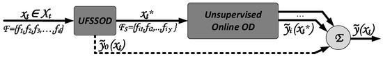
Figure 2. Conceptualization of module interaction for unsupervised FS for OD on SD (sequential approach).

The moving average ${\mu }_t$ and standard deviation ${\sigma }_t$ of the outlier scores until time t are obtained by applying, e.g., the well-known Welford’s algorithm [55] or one of the methods proposed in [13]. Scaling is necessary when combining algorithms of different nature with different characteristics. For instance, operating Loda_{Two Hist.} with different window sizes will result in different averaged score values due to the different state of knowledge on normal data. With increasing window sizes, the model becomes more accurate while seeing larger amounts of normal data, which are then scored less compared to models obtained from smaller window sizes. With the mean and standard deviation proportion of the Gaussian Scaling this difference will be eradicated and with the Error Function the scores are tailored to the interval between 0 and 1. With the normalized outlier scores, a final score can be computed, which might also be weighted. The confidence level of the Unsupervised Online OD module is typically higher than those of UFSSOD, since it operates on the reduced representation of a sample ${\mathit{x}}_t^{*}$ and thus one might give a higher weight to its score. For this, Equation (4) can be used depending on the weights $g_0$ for UFSSOD and $g_i$ for each classifier (typically $g_i>g_0$) where $g_0+{\sum }_i{g}_i=1$ and $\tilde{y}\in [0,1]$ applies. Using domain expertise, a reasonable threshold can be determined over runtime, yielding a decent classification performance that assigns a binary value from the set $\{normal,abnormal\}$ for each $\tilde{y}$.

$$\tilde{y}=g_0{\tilde{y}}_0+\sum _{i=1}^m{g}_i{\tilde{y}}_i$$

(4)

Since the UFSSOD module is able to provide different feature scores at each time step t, resulting in possible other top-$\gamma$-features than at time $t-i$, the downstream applied Unsupervised Online OD module might be capable of dealing with those changing features. If this is the case, the setup can truly work online, meaning that UFSSOD provides an updated version of the feature subset $F_S$ with a potentially changing cardinality that is used by the Unsupervised Online OD module to detect outliers in each t. To the best of our knowledge, only xStream is able to handle this situation. Moreover, xStream not only handles a varying cardinality of the feature subsets but is also able to deal with completely newly occurring features. However, the latter is not the focus of this work since for domain specific applications features are assumed to be known beforehand. Since most of the state-of-the-art unsupervised OD algorithms are operating on a fixed set of features with a fixed cardinality, a windowed approach can be utilized if the subsequently applied online OD algorithm is able to dynamically change its model during runtime. Thus, it can replace the old feature subset with the newly proposed one after the current time window elapsed. Possible algorithms would be iForest_ASD, which rebuilds its forest after a certain condition is met, thus also allowing to rebuild it with a different feature subset, or Loda_{Two Hist.} and HS-Trees using windowing where models are replaced with the ones currently built and the ones that will be built can use the current feature subset. With respect to Loda_{Two Hist.}, the old histograms built and classified with ${\mathcal{F}}_{S(t-i)}$ will be replaced with the new histograms using ${\mathcal{F}}_{S\left(t\right)}$, also allowing to change the cardinality (different top-$\gamma$-features).

If this sequential operation limits the throughput, a parallel approach can be utilized where both modules UFSSOD and Unsupervised Online OD work in parallel. As depicted in Figure 3 the online OD algorithm for each t operates with the previously proposed subset ${\mathcal{F}}_{S2}$, while the UFSSOD module continuously proposes a new ${\mathcal{F}}_S$, which is stored within ${\mathcal{F}}_{S1}$. The Unsupervised Online OD module can now decide whether it changes its feature subset for each t by using the one proposed by UFSSOD in $t-1$ switching between ${\mathcal{F}}_{S1}$ and ${\mathcal{F}}_{S2}$ or switching subsets again in a windowed fashion. The latter seems more convenient if the setup must not truly work online since the OD algorithm can work with the full throughput using the static feature subset until its model gets replaced or updated with the new subset, which was generated within the current time window. Furthermore, it should be noted that ufssod_clustering with respect to Algorithm 2 must not necessarily be performed for each sample in order to preserve resources while operating in the windowed mode. Thus, continuously ufssod_scoring is performed but ufssod_clustering is only performed if the subsequent classifier demands a new feature subset. With respect to Loda_{Two Hist.} and Figure 3, the old histograms built and classified with ${\mathcal{F}}_{S2}$ will be replaced with the new histograms switching to ${\mathcal{F}}_{S1}$ when the window size is reached, whereas UFSSOD continuously updates ${\mathcal{F}}_{S1}$ until switching.

Algorithm 2: Scoring functionality of UFSSOD—ufssod_scoring().

Input: A sample ${\mathit{x}}_t$ Output: The scaled outlier score ${\tilde{y}}_0$ and the averaged feature scores ${\overline{\mathit{s}}}_f$ 1  $y_0,{\mathit{s}}_f\leftarrow$ Loda_cont.update_score(${\mathit{x}}_t$) 2  ${\mu }_t\leftarrow$ outlier_score.moving_mean($y_0$) 3  ${\sigma }_t\leftarrow$ outlier_score.moving_sd($y_0$) 4  ${\tilde{y}}_0\leftarrow$ argmax(0, erf($\frac{y_0-{\mu }_t}{{\sigma }_t\sqrt{2}}$)) 5  ${\overline{\mathit{s}}}_f\leftarrow$ feature_scores.moving_mean($s_f$) 6  return${\tilde{y}}_0,{\overline{\mathit{s}}}_f$

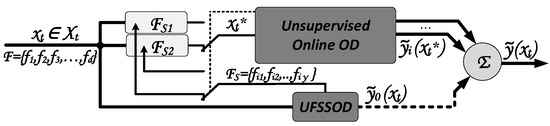
Figure 3. Conceptualization of module interaction for unsupervised FS for OD on SD (parallel approach).

4.3. Model for Scoring and Clustering Features

In this section, details of the internal working of UFSSOD (Figure 1) with regard to the core modules, ufssod_scoring() and ufssod_clustering(), is provided. Motivated by the functionality of Loda to rank features according to their contribution, UFSSOD leverages an adapted version of Loda_Cont. that continuously processes the feature scores for ranking and proposing the top-$\gamma$-features. Besides, it is able to provide outlier scores for each incoming ${\mathit{x}}_t$. It fulfills all the requirements of FS for SD and OD stated in Section 3.1. Also encouraged by IBFS, which exploits the training process of iForest for FS, we aimed to bring the nature of an online OD algorithm into this field as well but for the SD context. However, Loda seems more appropriate since it handles high-dimensional data more efficiently and is able to handle concept drifts. We see ourselves validated in our approach, since the evaluations of [14] prove that projection-based methods, as is the case with Loda, are advantageous in high dimensions with many irrelevant features, because the features relevant for OD are less likely to be selected by other methods that operate with $\mathcal{F}$. Therefore, sorting out those irrelevant features from high-dimensional data will significantly aid other OD methods by increasing their performance. Furthermore, the author of Loda already showed the capability of the algorithm to identify meaningful features in his experiments.

Our basis for Loda_Cont. is the Appendix: online histogram stated in [52]. However, it must be noted that both of its Algorithms 3 and 4 contain minor mistakes. In the former $z_{max}$ is computed by the $min$ instead of the correct $max$ function and referring to the latter, the formula for the probability $p\left(z\right)$ should depend on a weighted average of the bin counts. With the formula given, one obtains negative results in the case for negative $z_i$ and $z_{i+1}$. A corrected version has also been proposed by [56] such that for instance if z is closer to $z_i$, $p\left(z\right)$ gets weighted closer to $p\left(z_i\right)$ accordingly (Equation (5)).

$$p\left(z\right)=\frac{(z_{i+1}-z)m_i+(z-z_i)m_{i+1}}{M(z_{i+1}-z_i)}$$

(5)

Algorithm 3: Feature clustering of UFSSOD—ufssod_clustering().

The one-tailed two-sample t test has been proposed by the author of Loda, referring to Equation (4) in [52] to measure the statistic significance of each feature to its contribution of a sample’s anomalousness. Apart from the complexity of Loda_Cont. in time with $\mathcal{O}\left(h{d}^{-\frac{1}{2}}\right)$ and space $\mathcal{O}\left(h(d^{-\frac{1}{2}}+b)\right)$, referring to the naïve implementation of continuously updated histograms where h is the number of histograms and b the number of histogram bins, the identification of relevant features does not increase the complexity. This is because the statistical test performed is linear with respect to the number of projections h and number of features d and only increases the complexity in big $\mathcal{O}$ notation by a negligible constant [52]. We have integrated the functionality of relevant feature identification of Loda_Cont. in UFSSOD as a fundamental part and are able to produce feature scores $s_{fi\left(t\right)}$ for the ith feature $f_i$ at each time step t for one sample ${\mathit{x}}_t$, resulting in a one-dimensional array ${\mathit{s}}_f=\{s_{f1},s_{f2},...,s_{fd}\}$ of d feature scores per sample. Similarly to the continuous updating of the histograms, we propose to continuously update the feature scores for each sample by incremental averaging. There are various approaches discussed in [13], e.g., Exponentially Weighted Moving Average, that are better able to cope with occurring concept drifts in the feature scores while incrementally averaging them. As of now, however, we apply the incremental average as given per Equation (6) with a continuous counter value $n_t$ for each new data instance, in order to obtain the averaged array of feature scores ${\overline{s}}_f$ but reserve the right to use more advanced moving methods in future work. While only preserving d values for the current average scores, one value for the continuous counter $n_t$ and performing d updates of the scores, both the space and time complexity for each feature score averaging is $\mathcal{O}\left(d\right)$ when applying Welford’s algorithm. This does not significantly increase the overall complexity of UFSSOD since d is fixed. A summary of the scoring functionality of UFSSOD for both the outlier score and the feature scores, inclusive of their processing, is shown in Algorithm 2.

$${\overline{s}}_{fi\left(t\right)}=\frac{1}{n_t}({\overline{s}}_{fi(t-1)}{n}_{t-1}+s_{fi\left(t\right)})$$

(6)

Since the features within the subset are not only influencing the efficiency of the OD task but also the cardinality of the set significantly, the number $\gamma$ referring to the top-features is crucial. However, this is an optimization problem where the intention is to optimize the solution in such a way that the highest accuracy can be reached together with the lowest execution time achieved, e.g., by a smaller number of features. According to [8] it is still a challenging and known problem to determine the optimum number of features to select. Since this mostly applies for the supervised and offline case, we are stating that finding an optimal solution and therefore a point of equilibrium between the best classification with the lowest computational performance is impossible in the online setting.

When the Unsupervised Online OD module demands a new subset of the top-$\gamma$-features, UFSSOD clusters ${\overline{s}}_f$ to obtain the cluster(s) with the top scoring features. Even if clustering in one-dimensional space is not as trivial as it sounds, some algorithms are capable of solving this task, e.g., by applying Kernel Density Estimation (KDE), having a strong statistical background and seeking for local minima in density to split the data into clusters. However, we are proposing the k-mean adaption for one-dimensional clustering Ckmeans.1d.dp [57,58]. It achieves $\mathcal{O}\left(kd\right)$ by the optimization proposed in [58] for both time and space complexity, where k refers to the number of clusters built. Three improvements have been made for Ckmeans.1d.dp for the application within UFSSOD. We have (i) increased the factor of the Log-Likelihood within the BIC (Bayesian Information Criterion) computation, relevant to finding the optimum number of clusters k in order to better cluster the feature scores by more distinct spacing between data points. To avoid the case of too few feature scores in the top cluster yielding a small $\gamma$, we (ii) add a minimum constraint of having at least ${\gamma }_{min}$ feature scores in the top cluster. Thus, Ckmeans.1d.dp is performed as long as $|cluste{r}_1|\ge {\gamma }_{min}$ by successively reducing k starting from the initial optimum number of clusters $k_{opt}$. This adds a negligible constant to big $\mathcal{O}$ notation in the worst case where $|cluste{r}_1|=1$ of ${\gamma }_{min}-1$. For ${\gamma }_{min}$, we are proposing a minimum number of $\lceil \sqrt{d}\rceil$ features, which is often used as a rule of thumb for selecting features and achieved promising results in our evaluation. However, ${\gamma }_{min}$ can also be freely set by the domain expert. Since ${\gamma }_{min}$ only states the least requirement and the second, third, etc. best clusters might have promising feature scores as well. We are (iii) also proposing to check the distances between the cluster centers and their radii, which are defined by the utmost feature score from the cluster center as depicted with semicircles in Figure 4. Thus, not only the features of the cluster with the top scoring features $cluste{r}_1$ are returned, with $|cluste{r}_1|\ge {\gamma }_{min}$, but also those where the distance between the centers of $cluste{r}_i$ and $cluste{r}_{i+1}$ is less than the sum of radii of $cluste{r}_i$ and $cluste{r}_{i+1}$. Within the example of Figure 4 for $d=20$, $\lceil \sqrt{d}\rceil =5$, $|cluste{r}_1|=6$ the feature scores of $cluste{r}_1$ are returned with (ii) and $\gamma =6$ whereas those of $cluste{r}_1$ + $cluste{r}_2$ are returned with (iii) and $\gamma =11$.

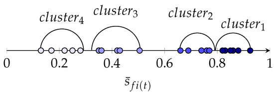
Figure 4. Visualization aid of ufssod_clustering with four exemplary clusters and semicircles around the cluster centroids.

It is again noted that the cardinality has a significant impact on the classifier since some even perform well with only a few features [26,51] whereas others operate best in high dimensions [14] or fluctuate with a varying number of relative features [52]. However, depending on the classifier used, one might adapt ${\gamma }_{min}$ or not use the cluster approach at all by setting $\gamma$ to a certain value. UFSSOD then ranks the feature scores in descending order, e.g., by the widely accepted Quick Sort or Merge Sort algorithm, and returns the top-$\gamma$-features. Depending on the chosen setup, in terms of complexity, we propose Merge Sort since the space and time complexity of d feature scores, even in the worst case, is $\mathcal{O}\left(d\right)$. A summary of the clustering functionality of UFSSOD is shown in Algorithm 3.

5. Evaluation

This section gives a glance at the experimental setup used for evaluation. First the test environment is presented, followed by information on the dataset collection used and a description of the evaluation methodology.

5.1. Test Environment

Experiments were conducted on a virtualized Ubuntu 20.04.1 LTS equipped with 12 x Intel(R) Xeon(R) CPU E5-2430 at 2.20 GHz and 32 GB memory running on a Proxmox server environment. All programs are coded in Python 3.7. Unless otherwise stated, commonly used Python libraries, e.g., numpy, are used for instance with the argsort function applying Merge Sort to sort the feature scores. We implemented ufssod_clustering in Python according to Ckmeans.1d.dp [58] with only the relevant functions for BIC and the one-dimensional cluster-routine and adapted it with respect to Section 4.3. As of now, however, we did not implement the return of additional clusters based on the cluster center distance verification.

For FS, we integrated the code (https://github.com/takuti/stream-feature-selection, accessed on 11 February 2021) for FSDS [28] and implemented IBFS according to the original paper [46] in the code (https://github.com/mgckind/iso_forest, accessed on 11 February 2021) of iForest. UFSSOD has been implemented according to Section 4.3 in Python as well.

For online OD on SD, we have chosen six off-the-shelf ensemble algorithms. Most of them have been shown to outperform numerous standard detectors [59]. The Python framework called PySAD (https://pypi.org/project/pysad/, accessed on 19 February 2021) (Python Streaming Anomaly Detection) proposed in [60] is used to provide multiple implementations for online/sequential anomaly detection. It contains among others RS-Hash [61], HS-Trees [62], iForest_ASD [53], Loda [52], Kitsune [63] and xStream [14]. However, some of them are not yet fully implemented, e.g., iForest_ASD, or their offline (batch) implementation is included, taken from PyOD [64], rather than their online counterparts as for Loda and xStream. Thus, we integrated RS-Hash, HS-Trees, and Kitsune from PySAD and used our own Python implementation of Loda_{Two Hist.}. We have avoided the use of the Rozenholc formula, stated by [52], to obtain the optimum number of bins per histogram and used default numbers of histograms and bins for all runs. Furthermore, iForest_ASD from scikit-multiflow [11] and the iMForest implementation (https://github.com/bghojogh/iMondrian, accessed on 19 February 2021) provided along with [48] was added for the online case. However, iForest_ASD was not included in the measurements due to (i) the lack of properly setting the drift threshold depending on the used datasets, which led to intense time-consuming measurements, and (ii) our desire to rely on the more advanced and recent iForest streaming competitor iMForest. xStream was taken from the StreamAD library (https://pypi.org/project/streamad/, accessed on 19 February 2021) providing the streaming version rather than the static one, as with PySAD. Unless otherwise stated, the default hyperparameters of the algorithms have been used and outlier thresholds have been fixed for all measurements. In order for the classifiers not to start their classification with empty models, all measurements are first initialized by processing 40% of the same input data later used for classification. This approach seems legitimate to us since we do not focus on the actual performance of each individual online OD classifier but rather want to evaluate the impacts of FS to them.

In terms of evaluation metrics, for each measurement, we computed the typical parameters of the confusion matrix for binary classification, True Negatives ($TN$), False Negatives ($FN$), False Positives ($FP$), and True Positives ($TP$) to derive the harmonic mean of precision and recall, denoted as the $F1$ score. It represents the classification performance of an algorithm and can be computed by Equation (7). Compared to other work that relies on the ROC (Receiver Operating Characteristic Curve), AUC (Area under the ROC), or only accuracy metric, e.g., [34,36,46], we see that the $F1$ score is more appropriate for OD since, e.g., the false positive rate used in the ROC metric depends on the number of $TN$, whose proportion in OD is typically quite large. Hence, the ROC curve tends to be near 1 when classifying imbalanced data and thus is not the best measure for examining OD algorithms. A good $F1$ indicates low FP and FN and is therefore a better choice to reliably identify malicious activity in the network security domain without being negatively impacted by false alarms.

$$F1=\frac{TP}{TP+\frac{1}{2}(FP+FN)}$$

(7)

Furthermore, we have measured the average runtime per OD algorithm, denoted as $avg\_t$, as a representative metric for the computational performance. Thus we accumulated the elapsed time for individual steps necessary to perform, e.g., partial fitting or prediction to derive the average runtime after multiple iterations for processing a particular dataset. Having a tradeoff between the classification and computational performance, the third metric is the ratio of $F1/avg\_t$.

5.2. Data Source

Rather than relying on a security-domain specific single dataset such as KDD’99, NSL-KDD or a predestined younger one CSE-CIC-IDS2018 (https://registry.opendata.aws/cse-cic-ids2018/, accessed on 5 March 2021), we have deliberately chosen real-world candidate datasets from the ODDS (http://odds.cs.stonybrook.edu/about-odds/, accessed on 5 March 2021) (Outlier Detection DataSets) Library [65] which are commonly used to evaluate OD methods for various reasons. In recent years, the majority of state-of-the-art IDS datasets have been criticized by many researchers since their data is out of date or do not represent today’s threat landscape [51,66,67]. Even if CSE-CIC-IDS2018 overcomes some shortcomings, it was not optimal for the extensive number of measurements performed (Figure 5) due to its enormous number of data instances in multiple files. Furthermore, we wanted to stress test UFSSOD with very dynamic datasets, meaning that outliers might occur in various features, which are typically not the same. As could be shown with its predecessor, the CICIDS2017, only a subset of three to four features per attack is enough to describe it best [51], making it look quite static. With an ensemble of the 15 datasets from ODDS shown together with their characteristics in Table 3, we have focused on a variety of datasets in terms of length, dimension, and outlier percentage from multidisciplinary domains. Except for lympho and vertebral, which have been neglected due to their insignificant number of data instances or dimensions, those datasets are also used by PyOD for benchmarking. Furthermore, to reduce the processing runtime of each OD algorithm we truncated mnist, musk, optdigits, pendigits, satellite, satimage-2, and shuttle while mostly maintaining its outlier percentage.

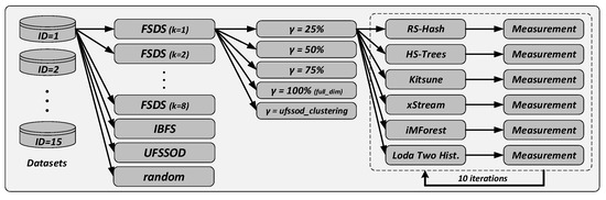
Figure 5. Flowchart of the evaluation measurements.

Table 3. Characteristics of the utilized and partially adapted datasets from ODDS [65].

ID	Dataset	# Instances	# Dimensions	Outliers (%)
1	arrhythmia	452	274	14.6
2	cardio	1831	21	9.6
3	glass	214	9	4.2
4	ionosphere	351	33	35.9
5	letter	1600	32	6.25
6	mnist	2603	100	26.9
7	musk	1000	166	9.7
8	optdigits	2216	64	6.8
9	pendigits	2000	16	2.3
10	pima	768	8	34.9
11	satellite	3000	36	31.1
12	satimage-2	1750	36	1.0
13	shuttle	3000	9	7.9
14	vowels	1456	12	3.4
15	wbc	378	30	5.6

5.3. Evaluation Methodology

For the comparison of FSDS and IBFS, as representatives of FS for SD and OD, with UFSSOD, our methodology is shown in a flow chart in Figure 5. For each dataset of Table 3 we have performed extensive measurements by first setting an FS algorithm. It must be noted that FSDS is relying on the number of singular values k. The authors of FSDS state that this parameter should be equal to the number of clusters in the dataset. However, since our focus is on classification rather than on clustering, we have performed measurements with different values for k to test the applicability of FSDS for OD. After the FS algorithms yield their scores for each feature, the subset is obtained by different $\gamma$, e.g., the top 25% ranked features, randomly chosen $\gamma$ features, or automatically proposing $\gamma$ features by using ufssod_clustering to avoid the top-$\gamma$-problem. Each obtained subset has been used by six online capable OD algorithms per measurement yielding $avg\_t$ and $F1$ per classifier. Finally, the results have been averaged across 10 independent runs, since most of the methods are non-deterministic, e.g., negatively affected by random projection.

Since no other unsupervised FS algorithms for OD with regard to a streaming fashion exist, we have tested our conceptualization in the two proposed settings of Figure 2 and Figure 3. Thus, we let UFSSOD compute an outlier score and propose the top-$\gamma$-features for each data instance that will immediately be used and processed sequentially by xStream. For Loda_{Two Hist.} we have used the parallel approach and let Loda build histograms using the current feature subset while classifying with the old one. The window size was set to 200 samples rather than 256 used by [52] because of the limited number of data instances in the glass dataset. After the window size is reached, the current classifying histograms are replaced with the ones built and the new histograms are built using the currently proposed subset by UFSSOD. The streaming setting was only performed on the datasets with IDs 2, 5, 6, 8, 9, 11, 12, 13, and 14 due to their more meaningful number of data instances for a streaming setting. Since we stick to the default threshold values for most of the classifiers and do not extract the score values but their binary prediction, we have not utilized the scaled combination approach so far. Despite that, we have combined the results of UFSSOD, xStream, and Loda_{Two Hist.} by a simple logical or-conjunction in three settings: UFSSOD with xStream, UFSSOD with Loda_{Two Hist.} and UFSSOD with xStream with Loda_{Two Hist.} as a combination of UFSSOD with two downstream applied OD algorithms. Although achieving a higher $TP$ while also producing more $FP$, our approach is legitimate under the assumption that it is more important to detect attacks while coping with $FP$ in a consecutive alert analysis. Albeit not within the scope of this work, it must be noted that most of the classifiers are not able to perform root cause analysis, e.g., Kitsune as stated in [68], which might be relevant for a subsequent alert analysis.

6. Discussion of Results

In this section we discuss some of the key results obtained by the comprehensive evaluation. We have structured this section into three parts. First we discuss the applicability of FSDS as an FS algorithm for SD when utilized for the purpose of OD by comparing it with IBFS and UFSSOD. Then, IBFS as an FS algorithm for OD is compared with UFSSOD in different feature subset settings to discuss the comparable operational capability of UFSSOD as an FS algorithm for OD. Lastly, we prove the applicability of UFSSOD in conjunction with the online OD algorithms xStream and Loda_{Two Hist.} in two different streaming settings.

6.1. Comparison of FSDS, IBFS and UFSSOD with the Best 25% Features

First, we compare the results for $\gamma$ set to the 25% of the top-ranked features for FSDS, IBFS, and UFSSOD. The reason behind only considering the top 25% is that if the FS algorithm is able to rank the features according to their contribution of anomalousness properly, the results should, even with this limited amount of features, be noticeable for the task of OD. If one of the FS algorithms yielded poor results even for the top features, we could show its non-applicability to the task of OD. The results of the $F1/avg\_t$ metric are shown in Table 4. We have chosen the $F1/avg\_t$ metric in this setup since, independently of IBFS being an offline FS algorithm, we wanted to include the information of the tradeoff between classification and computational performance, especially to compare FSDS with UFSSOD, being of online nature. Since we have also compared feature subsets of the same cardinality, this approach is legitimate. Nevertheless, the results for $F1$ show a similar behavior. It is noted that FSDS is able to process more than only one sample at each time t. The implementation used, required 10 samples at each time to function properly. Thus, the results, with regard to $avg\_t$, would be even worse for FSDS if it only processed 1 instead of 10 samples due to a longer runtime.

Table 4. $F1/avg\_t$ results for FSDS (different k), IBFS, and UFSSOD for $\gamma$ set to 25% of d for datasets with ID i (values are scaled with $\times {10}^{-3}$ and in unit 1/s, best performing feature set in bold).

ID	FSDS_k_1	FSDS_k_2	FSDS_k_3	FSDS_k_4	FSDS_k_5	FSDS_k_6	FSDS_k_7	FSDS_k_8	IBFS	random	UFSSOD
1	10.01	10.35	10.28	9.92	9.97	10.11	9.97	9.99	11.27	8.18	9.89
2	2.41	2.03	2.21	1.55	1.62	1.71	1.77	1.71	2.83	2.24	2.58
3	7.30	7.92	6.40	9.36	7.21	11.00	8.80	9.39	12.20	6.88	3.30
4	17.19	19.52	18.76	18.26	18.17	18.94	18.34	17.61	18.55	18.47	18.99
5	1.36	1.42	1.41	1.40	1.06	1.16	0.88	1.21	1.39	1.15	1.32
6	2.01	2.11	2.07	2.18	1.99	2.02	2.31	2.46	1.77	1.69	1.81
7	6.43	6.95	8.56	8.86	7.12	6.20	5.02	5.10	7.75	6.62	6.49
8	1.39	1.36	1.16	1.41	1.30	1.31	1.41	1.88	0.68	0.54	0.68
9	0.93	0.85	0.68	0.63	0.67	0.49	0.51	0.55	0.63	0.78	0.61
10	7.02	7.06	6.15	7.32	6.11	5.45	6.39	8.81	7.84	7.41	8.91
11	1.58	2.20	2.01	2.01	2.40	2.12	2.17	2.05	3.21	2.00	3.17
12	0.54	0.39	0.51	0.60	0.59	0.62	0.67	0.56	1.26	0.58	0.95
13	1.08	0.70	0.59	1.93	1.65	1.40	1.66	1.24	1.24	0.76	2.82
14	0.60	0.66	0.73	0.80	0.86	1.09	1.00	0.64	1.64	0.97	1.23
15	13.39	12.40	11.17	10.55	11.05	12.97	12.73	10.51	25.75	11.47	24.84

Surprisingly, for some datasets, FSDS performs comparably or even better than IBFS or UFSSOD. However, for those datasets even randomly choosing 25% of d features perform mostly comparable as well and the better $F1/avg\_t$ is mostly explained by the better average runtime of FSDS compared to IBFS and UFSSOD, especially for datasets with a high dimension. For instance, with musk ($d=100$), IBFS and UFSSOD have an approximately 29% higher runtime compared to all FSDS subset results. For better comprehensibility, two exemplary plots of the $F1$ for letter and musk are shown in Figure 6 where IBFS and UFSSOD performed poorly and FSDS achieves better results. For letter in Figure 6a, the overall $F1$ is quite poor, also showing that randomly choosing 25% of features achieves results comparable to the other subsets. It is due to the nature of both IBFS and UFSSOD, being based on an OD algorithm, that if the overall $F1$ is poor, to not reliably score the feature contributions with regard to their anomalousness. With an overall decent $F1$ achieved by the subsets in musk (Figure 6b), one can clearly see that IBFS and UFSSOD perform significantly better than the random subset and for most of the FSDS subsets with different k.

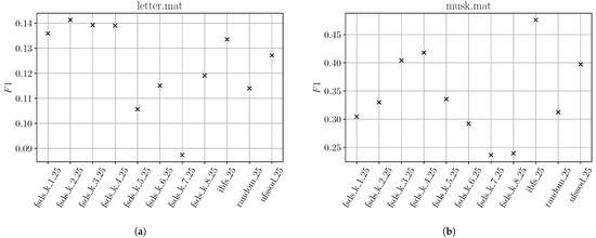
Figure 6. Exemplary $F1$ plots for badly-performing IBFS and UFSSOD using top 25% feature subsets on datasets letter (a) and musk (b).

Figure 7 shows the $F1$ results of datasets where IBFS and UFSSOD performed well and an overall decent $F1$ could be achieved. In all subfigures it can be seen that both IBFS and UFSSOD achieved better results than randomly selecting 25% of features, proving that even for this fixed small amount of features, IBFS and UFSSOD are able to score features reliably according to their contribution of anomalousness. Two key outcomes can be noted. First, in most of the cases FSDS could not achieve better results than randomly selecting features while IBFS and UFSSOD are able to produce better ones. Second, independent of the used parameter k, the results significantly vary for each k per dataset without any pattern apparent, e.g., the smaller the dimension the smaller the k. Even if promising results can occasionally be obtained for some k, without any pattern behind, one is not able to properly set the parameter. Those individual cases, e.g., in Figure 7d with FSDS and $k=1$, might be explained by FSDS’ ability to find redundancy among features in a higher dimension, which scored worse and coincidentally might not contain any outliers. Thus, their removal will positively affect the $F1$. However, this way of sorting out irrelevant features is not the actual intention of FS for the task of OD.

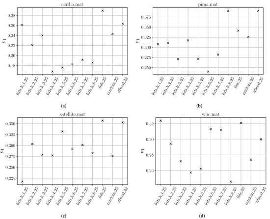
Figure 7. Exemplary $F1$ plots for well-performing IBFS and UFSSOD using top 25% feature subsets on datasets cardio (a), pima (b), satellite (c) and wbc (d).

To find an explanation for the worse performance of IBFS and UFSSOD compared to FSDS in terms of $F1/avg\_t$ for some datasets, we have examined two exemplary ones: musk (Figure 6b) as a representative for the badly-performing and satellite (Figure 7c) for the well-performing with decent $F1$ scores. We then examined the plotted feature scores of both, which are depicted in Figure 8. It can clearly be seen in Figure 8a and especially in Figure 8b that the majority of scores lies densely within a certain range and is homogeneously distributed, which is an indicator that outliers tend to occur in any feature. Referring to Figure 8c and especially Figure 8d, a more heterogeneous distribution of the feature scores for the satellite dataset can be seen, reasoning that outliers might tend to occur in the same features, which generally contribute more to the outlier score.

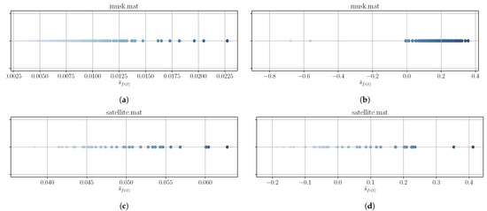
Figure 8. Exemplary plots for feature scores ${\overline{s}}_{fi\left(t\right)}$ of IBFS (a,c) and UFSSOD (b,d) applied on musk (a,b) and satellite (c,d) (the more intense the color, the higher the score, and the more important the feature).

6.2. Comparison of IBFS and UFSSOD with Different Feature Sets

Since FSDS did not prove to be a promising candidate for OD, we have proceeded our result discussion by comparing IBFS and UFSSOD. Because of applying different feature set lengths and an offline with an online algorithm, we now focus on the results of the $F1$ metric for different subsets, as shown in Table 5, since we do not want to blur results with shorter average runtimes. For only two datasets, optdigits and satellite, using all features is more promising whereas, for optdigits, the feature subsets perform much worse. For satellite the $F1$ scores across all columns are comparable.

Table 5. $F1$ results for IBFS and UFSSOD for different $\gamma$ (feature subsets) for datasets with ID i (full_dim refers to using all features $\gamma =d$, *_25,50,75 refers to setting $\gamma$ to the top scoring 25, 50, and 75% features and *_ckm refers to the top-$\gamma$-features obtained by ufssod_clustering, best performing feature set in bold).

ID	full_dim	ibfs_25	ibfs_50	ibfs_75	ibfs_ckm	ufssod_25	ufssod_50	ufssod_75	ufssod_ckm
1	0.279	0.305	0.290	0.277	0.308	0.274	0.282	0.286	0.266
2	0.295	0.297	0.284	0.293	0.296	0.261	0.298	0.297	0.264
3	0.092	0.158	0.090	0.110	0.090	0.054	0.062	0.138	0.060
4	0.470	0.408	0.458	0.491	0.398	0.409	0.438	0.472	0.459
5	0.129	0.137	0.134	0.141	0.120	0.124	0.113	0.115	0.123
6	0.271	0.266	0.295	0.319	0.312	0.340	0.303	0.344	0.312
7	0.359	0.482	0.435	0.420	0.463	0.404	0.420	0.404	0.411
8	0.158	0.079	0.096	0.138	0.092	0.086	0.083	0.099	0.065
9	0.101	0.072	0.094	0.090	0.060	0.072	0.097	0.097	0.102
10	0.350	0.345	0.245	0.351	0.248	0.390	0.234	0.327	0.348
11	0.364	0.354	0.297	0.306	0.292	0.352	0.300	0.339	0.347
12	0.061	0.067	0.075	0.067	0.064	0.056	0.073	0.064	0.058
13	0.395	0.113	0.303	0.406	0.447	0.260	0.341	0.340	0.397
14	0.093	0.075	0.096	0.109	0.095	0.057	0.098	0.091	0.097
15	0.283	0.321	0.292	0.249	0.305	0.302	0.293	0.273	0.310

A better picture of the bad performance for optdigits can be made by examining the feature scores ${\overline{s}}_{fi\left(t\right)}$, as shown in Figure 9. The red crosses mark those features that are returned by ufssod_clustering applied on the scores of IBFS and UFSSOD. From a number of 64 features for full dimension, ufssod_clustering applied on IBFS and UFSSOD only marks 9 features to be the most important. Since for optdigits it generally applies that the higher the number of features in the subset the better the score, even the measurements with 75% of features seems not sufficient enough. Again, this is supporting the assumption that for optdigits outliers tend to occur in any feature. An overall $F1$ of only 0.158 by using all features shows that the online OD algorithms also performed quite poorly on this dataset.

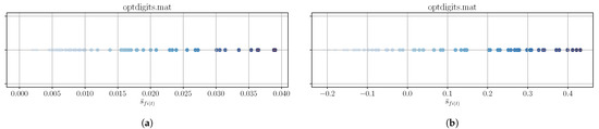
Figure 9. Exemplary plots for feature scores ${\overline{s}}_{fi\left(t\right)}$ of IBFS (a) and UFSSOD (b) applied on optdigits (the more intense the color, the higher the score, and the more important the feature; red crosses mark the top-$\gamma$-features by ufssod_clustering).

Even if IBFS and UFSSOD with the ufssod_clustering subset performed approximately 7% faster with regard to $avg\_t$, considering the $F1/avg\_t$ metric for all subsets depicted in Figure 10, it did not significantly influence the results at all.

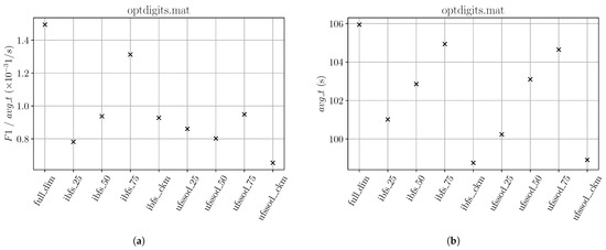
Figure 10. $F1/avg\_t$ (a) and $avg\_t$ (b) results for optdigits referring to Table 5.

Independently of whether using IBFS or UFSSOD, in the majority of cases using a subset of features performs better than using the full set. For better comprehensibility, two exemplary plots for datasets that have achieved decent $F1$ scores are shown in Figure 11. In Figure 11a, it can be seen that using all 100 features of the mnist dataset degrades the classification performance, whereas ufssod_clustering with 37 (IBFS) and 21 (UFSSOD) features achieved very good results in terms of $F1/avg\_t$. For UFSSOD, slightly more features as shown with the 25% measurement would have achieved even better results. Figure 11b shows the results for the wbc dataset and that it is not always better to choose a high percentage of top scoring features. From the 30 features in total, using ufssod_clustering with 10 (IBFS) and 14 (UFSSOD), features achieved much better results than subsets with a higher number.

Figure 11. $F1/avg\_t$ results for well-performing datasets mnist (a) and wbc (b) referring to Table 5.

In order to show the influence of applying ufssod_clustering for IBFS or UFSSOD for each classifier, we refer to Table 6. As a representative example with the wbc dataset, the percentage increase or decrease of the metrics $avg\_t$ and $F1$ compared to the measurements using the full feature dimension is shown. For each classifier, applying ufssod_clustering, whether on IBFS or UFSSOD, could decrease the runtime by approximately 12% on average considering the significant improvement on Kitsune. The $F1$ score could be increased by approximately 14% on average. HS-Trees and Kitsune show a significant improvement and a slight improvement could also be noticed for Loda_{Two Hist.}, whereas iMForest and RS-Hash have shown a classification degradation. For xStream the application of UFSSOD even yielded an $F1$ improvement compared to IBFS.

Table 6. Individual classifier performance in terms of the percentage increase/decrease of $avg\_t$ and $F1$ applying ckeans_ufssod on IBFS and UFSSOD compared to full dimension on wbc dataset.

wbc ($\mathit{d}=30$)	$\mathit{\gamma }=10$ (ibfs_ckm)		$\mathit{\gamma }=14$ (ufssod_ckm)
	% $\mathit{avg}\_\mathit{t}$	% $\mathit{F}1$	% $\mathit{avg}\_\mathit{t}$	% $\mathit{F}1$
RS-Hash	−2.33	−1.04	−1.68	−4.24
HS-Trees	−1.14	64.97	−1.34	27.25
Kitsune	−68.89	56.86	−68.56	66.67
xStream	−1.90	−21.15	−1.62	3.23
iMForest	−0.08	−16.66	−0.34	−8.25
LodaTwo Hist.	−2.52	4.00	−1.33	1.20

6.3. Application of UFSSOD, xStream, and Loda Two Hist. in a Streaming Setting

Measurement results for the streaming setting with regard to the sequential and parallel approach (Figure 2 and Figure 3) are shown in Table 7. The $F1$ score results are averaged by the results of UFSSOD, xStream, Loda_{Two Hist.} and their logical or-combination stated in Section 5.3.

Table 7. $F1$ results for UFSSOD using different $\gamma$ (feature subsets) for datasets with ID i in streaming setting with xStream and Loda_{Two Hist.} (full_dim refers to using all features $\gamma =d$, *_25,50,75 refers to setting $\gamma$ to the top scoring 25, 50, and 75% features and *_ckm refers to the top-$\gamma$-features obtained by ufssod_clustering, best performing feature set in bold).

ID	full_dim	ufssod_25	ufssod_50	ufssod_75	ufssod_ckm
2	0.435	0.404	0.402	0.416	0.390
5	0.083	0.083	0.088	0.076	0.093
6	0.161	0.282	0.229	0.204	0.328
8	0.136	0.097	0.122	0.108	0.113
9	0.154	0.169	0.186	0.159	0.170
11	0.349	0.391	0.389	0.384	0.396
12	0.267	0.247	0.247	0.271	0.254
13	0.425	0.350	0.455	0.456	0.394
14	0.039	0.075	0.077	0.075	0.056

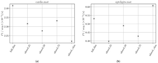
For only two datasets, cardio and optdigits, using all features achieved better classification performance than using a subset. However, instead of yielding worse results, the subsets performed comparably to the full set. Taking into account the average runtime decrease using a subset, as shown in Figure 12b, for optdigits, UFSSOD with ufssod_clustering even achieved a better tradeoff than the other settings. For cardio the $F1/avg\_t$ could not provide better results. The reason why ufssod_clustering has a higher influence on the result of the $F1/avg\_t$ metric on optdigits than on cardio is due to the fact that with only 21 (cardio) and 64 (optdigits) the number of dimensions can be reduced more significantly in the latter case. Therefore, the average runtime can also be reduced more notably. Since the $avg\_t$ of cardio with its minor number of features can be reduced only marginally with ufssod_clustering, the dominating factor remains the $F1$ score.

Figure 12. $F1/avg\_t$ results for badly-performing datasets cardio (a) and optdigits (b) referring to Table 7.

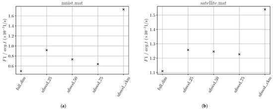
In three dataset measurements, letter, mnist and satellite, ufssod_clustering applied in a streaming setting to xStream and Loda_{Two Hist.} yielded the best results. We have neglected letter since the overall $F1$ score is poor across all feature sets and therefore the results are non-significant. For mnist, ufssod_clustering notably achieved the best $F1$ compared to the other feature sets, where even when using all features, it performed the worst. With mnist’s 100 dimensions, the good result is improved, shown in Figure 13a, considering the significant reduction of features resulting in a runtime decrease of approximately 40% and thus a better $F1/avg\_t$ metric. Even for satellite having only 36 dimensions, this effect takes place, shown in Figure 13b, where the $avg\_t$ is being decreased by approximately 20%.

Figure 13. $F1/avg\_t$ results for well-performing datasets mnist (a) and satellite (b) referring to Table 7.

In order to show the influence of applying UFSSOD to xStream and Loda_{Two Hist.}, we refer to Table 8 showing the percentage increase or decrease of the metrics $avg\_t$ and $F1$ compared to the measurements using the full feature set. For all datasets, xStream achieves better results with UFSSOD in terms of $avg\_t$ with an overall improvement of approximately 11% compared to the measurements using all features. However, with an average runtime per dataset (full dimension) of approximately 590 sec yielding 0.27 s/sample across all datasets, xStream’s Python implementation of StreamAD does not seem very efficient compared to our Loda_{Two Hist.} implementation, with approximately 3 s average runtime per dataset and 1.4 ms/sample. Compared to the other classifiers in the measurements, xStream was the only one with this significant runtime, also explaining why the authors of xStream provided a C++ streaming version rather than a Python pendant to their static one. Considering the fast runtime of Loda_{Two Hist.}, significant improvements of $avg\_t$ could only be achieved for datasets whose number of data instances and dimension ratio is higher (ID 6, 8, and 11) than those of the others and, on average, reduces $avg\_t$ by 7%. As an example, for optdigits with 2216 data instances and 64 dimensions, UFSSOD could reduce $avg\_t$ by approximately 22%. As for the percentage improvement of $F1$, excluding the statistical strays of dataset 6 and 15 for xStream, an improvement of approximately 22% on average could be obtained. For Loda_{Two Hist.}, the improvement is even more notable with approximately 45% (ID 6 and 15 excluded).

Table 8. Performance of xStream and Loda_{Two Hist.} in terms of the percentage increase/decrease of $avg\_t$ and $F1$ applying UFSSOD in a streaming setting compared to full dimension (N/A for ID 15 since no $F1$ score could be obtained with full dimension due to poor classification results).

ID	xStream		LodaTwo Hist.
	% $\mathit{avg}\_\mathit{t}$	% $\mathit{F}1$	% $\mathit{avg}\_\mathit{t}$	% $\mathit{F}1$
2	−2.74	−30.72	0.49	−6.41
5	−2.29	60.29	3.18	−14.37
6	−42.9	2638.80	−36.38	232.54
8	−28.4	−47.85	−22.22	305.52
9	−1.34	1.50	1.39	41.81
11	−18.75	34.63	−15.21	3.46
12	−3.19	111.16	1.82	−1.34
13	−1.70	22.61	1.68	−16.07
15	−1.15	N/A	0.29	16.00

It should be noted that xStream worked in the truly online mode. Therefore similar performance boosts, as with Loda_{Two Hist.}, might also be achieved for xStream if using the proposed windowed approach mentioned in Section 4. In summary, applying UFSSOD in a streaming setting notably increases both the classification and computational performance if the dataset is of high-dimensional nature and has a high number of data instances. In a real-world application, the former depends on the applied domain but fits perfectly with current observable trends. The latter is only part of this evaluation setup since in the real-world the data stream has an infinite amount of samples. Although xStream and Loda are representatives that work better on high-dimensional data [14] and one might assume that a reduction of features by UFSSOD might degrade their performance, the experiments show that the opposite is true, with an overall improved result. Thus, we assume that using UFSSOD with other online classifiers, such as ones based on iForest that handle changing feature sets during runtime, may boost the performance even more.

7. Conclusions and Future Work

In this work we have illuminated the necessity of unsupervised Feature Selection (FS) for Outlier Detection (OD) in Streaming Data (SD) for domains, e.g., intrusion detection, in network security, which are ever-increasingly facing high-volume and high-dimensional data that need to be processed in almost real-time. With the extensive review on FS approaches for either (i) SD or (ii) OD, we have pointed out that, to the best of our knowledge, the proposed Unsupervised Feature Selection for Streaming Outlier Detection, called UFSSOD, is the first method of its kind to fill the research gap by providing a solution bridging (i) and (ii). Two application scenarios of UFSSOD, together with online capable OD methods, are discussed along with UFSSOD’s operation and functionality. This also includes the ability to provide the amount of top-performing features by clustering their score values, which is often circumvented in the literature by setting a pre-defined number. Extensive measurements were conducted on 15 real-world datasets by applying multiple feature subsets to six widely accepted off-the-shelf online OD methods obtained from UFSSOD and state-of-the-art competitors FSDS as a representative of (i) and IBFS of (ii). The evaluation examines the alleviation of the negative effect brought by irrelevant features for the outlier detectors, considering both, the classification and computational performance. The discussion of the results pointed out the non-applicability of FSDS for OD because it does not achieve reliable and satisfactory results, independent of its cluster parameter k. In comparison to (offline) IBFS, UFSSOD achieves at least comparable results while operating in an online fashion. It was able to decrease the average runtime of individual classifiers by approximately 12% and improve the $F1$ by 14% on average. UFSSOD is also evaluated in a true online setting by providing a feature subset inline to xStream for each sample and to Loda_{Two Hist.} using a windowed approach. In this setting, applying UFSSOD yields better results than the bare versions of the OD methods operating on full dimension. For instance, UFSSOD could improve the $F1$ up to 45% for Loda_{Two Hist.} while reducing the average runtime by 22% for individual data sets.

As assumed, UFSSOD works better if the outliers in the dataset tend to occur in the same features, which is mostly the case, as stated, in the network security domain. Even passing the stress test on datasets that does not meet this presumption, as part of future work, UFSSOD will be thoroughly examined on more domain-specific datasets. Especially, the CSE-CIC-IDS2018 dataset allows to evaluate different types of features (e.g., flow or packet based) and their influence on the performance of UFSSOD. Instead of using existing datasets, we will apply UFSSOD in a real world computer network (no labeled data available) in parallel to classifiers without feature selection to examine the differences in classification results. A recently proposed method [69] might be applied to exploit and evaluate the outcome of outlier detection for novel attack pattern recognition on streaming data with and without the application of UFSSOD’s feature selection.

Since in the current configuration, measurements only relied on the ${\gamma }_{min}$ functionality with respect to Algorithm 3, a part of our future work will be comparing it with the $distance$ functionality, which tends to result in more features, leading to higher computational costs, but might improve the classification task even further. Additionally, a more thorough testing of the outlier scaling and its combination across multiple online detection approaches will be performed. In terms of UFSSOD’s operation modes, the discussion of results revealed inferior performance of xStream applied in the true online setting compared to Loda_{Two Hist.}’s windowed setting. Within the scope of our future work is also to apply xStream in the windowed setting and check which mode—sequential or parallel—is in general more effective and why. Since UFSSOD’s main purpose is the streaming feature selection for outlier detection, further evaluation should also include the latest online outlier detection methods, e.g., PCB-iForest [70].

Inspired by approaches used in CINFO or ODEFS and the nature of UFSSOD to provide outlier candidates, in future work we will examine the possibility of applying supervised FS, similarly to sparse Lasso regression in CINFO, based on pseudo-labels obtained from UFSSOD’s outlier candidates. Thus, not only the pure nature of Loda’s functioning will form the basis for FS but it may also be improved by shrinking the solution, resulting in a number of features that are not correlated to the outlier score. To even further alleviate the circumstance that FS is performed independently of the subsequent online OD method, possibly yielding a suboptimal and biased solution for OD, we might include outlier candidates from the Unsupervised Online OD module as well. Instead of performing iterative validations to reduce the loss in an offline setting having all data objects available, we will research possibilities to do so in a slimmed-down online fashion by exploiting the strength of theoretically infinite running time of SD.

References

- Hindy, H.; Brosset, D.; Bayne, E.; Seeam, A.K.; Tachtatzis, C.; Atkinson, R.; Bellekens, X. A taxonomy of network threats and the effect of current datasets on intrusion detection systems. IEEE Access 2020, 8, 104650–104675. [Google Scholar] [CrossRef]
- Sarker, I.H.; Kayes, A.S.M.; Badsha, S.; Alqahtani, H.; Watters, P.; Ng, A. Cybersecurity data science: An overview from machine learning perspective. J. Big Data 2020, 7, 41. [Google Scholar] [CrossRef]
- Mahfouz, A.; Abuhussein, A.; Venugopal, D.; Shiva, S. Ensemble classifiers for network intrusion detection using a novel network attack dataset. Future Internet 2020, 12, 180. [Google Scholar] [CrossRef]
- Pang, G.; Cao, L.; Chen, L.; Liu, H. Unsupervised feature selection for outlier detection by modelling hierarchical value-feature couplings. In Proceedings of the 2016 IEEE 16th International Conference on Data Mining (ICDM), Barcelona, Spain, 12–15 December 2016; pp. 410–419. [Google Scholar] [CrossRef]
- Thakkar, P.; Vala, J.; Prajapati, V. Survey on outlier detection in data stream. Int. J. Comput. Appl. 2016, 136, 13–16. [Google Scholar] [CrossRef]
- Moradi, P.; Gholampour, M. A hybrid particle swarm optimization for feature subset selection by integrating a novel local search strategy. Appl. Soft Comput. 2016, 43, 117–130. [Google Scholar] [CrossRef]
- Nguyen, H.T.; Petrović, S.; Franke, K. A comparison of feature-selection methods for intrusion detection. In Lecture Notes in Computer Science; Springer: Berlin/Heidelberg, Germany, 2010; pp. 242–255. [Google Scholar] [CrossRef]
- Li, J.; Cheng, K.; Wang, S.; Morstatter, F.; Trevino, R.P.; Tang, J.; Liu, H. Feature selection: A data perspective. ACM Comput. Surv. 2018, 50, 1–45. [Google Scholar] [CrossRef]
- Zöller, M.-A.; Huber, M.F. Benchmark and survey of automated machine learning frameworks. J. Artif. Intell. Res. 2021, 70, 409–472. [Google Scholar] [CrossRef]
- Krawczyk, B.; Cano, A. Online ensemble learning with abstaining classifiers for drifting and noisy data streams. Appl. Soft Comput. 2018, 68, 677–692. [Google Scholar] [CrossRef]
- Togbe, M.U.; Barry, M.; Boly, A.; Chabchoub, Y.; Chiky, R.; Montiel, J.; Tran, V.-T. Anomaly detection for data streams based on isolation forest using scikit-multiflow. In Computational Science and Its Applications—ICCSA; Lecture Notes in Computer Science; Gervasi, O., Ed.; Springer: Cham, Switzerland, 2020; Volume 12252, pp. 15–30. [Google Scholar] [CrossRef]
- Ahmad, S.; Lavin, A.; Purdy, S.; Agha, Z. Unsupervised real-time anomaly detection for streaming data. Neurocomputing 2017, 262, 134–147. [Google Scholar] [CrossRef]
- Reunanen, N.; Räty, T.; Jokinen, J.J.; Hoyt, T. Unsupervised online detection and prediction of outliers in streams of sensor data. Int. J. Data Sci. Anal. 2020, 9, 285–314. [Google Scholar] [CrossRef]
- Manzoor, E.; Lamba, H.; Akoglu, L. xStream: Outlier detection in feature-evolving data streams. In Proceedings of the 24th ACM SIGKDD International Conference on Knowledge Discovery & Data Mining; London, UK, 19–23 August 2018, ACM: New York, NY, USA, 2018. [Google Scholar] [CrossRef]
- Iglesias, F.; Zseby, T. Analysis of network traffic features for anomaly detection. Mach. Learn. 2015, 101, 59–84. [Google Scholar] [CrossRef]
- Zheng, A. Feature Engineering for Machine Learning; O’Reilly Media: Sebastopol, CA, USA, 2018; ISBN 9781491953242. [Google Scholar]
- Rahmaninia, M.; Moradi, P. OSFSMI: Online stream feature selection method based on mutual information. Appl. Soft Comput. 2018, 68, 733–746. [Google Scholar] [CrossRef]
- Almusallam, N.; Tari, Z.; Chan, J.; AlHarthi, A. UFSSF—An efficient unsupervised feature selection for streaming features. In Advances in Knowledge Discovery and Data Mining; Springer International Publishing: Cham, Switzerland, 2018; pp. 495–507. [Google Scholar] [CrossRef]
- Chapman, S.; Richard, Y.D.X. Diverse Online Feature Selection. arXiv 2019, arXiv:1806.04308v3. [Google Scholar]
- Panday, D.; Cordeiro de Amorim, R.; Lane, P. Feature weighting as a tool for unsupervised feature selection. Inf. Process. Lett. 2018, 129, 44–52. [Google Scholar] [CrossRef]
- Fahy, C.; Yang, S. Dynamic feature selection for clustering high dimensional data streams. IEEE Access 2019, 7, 127128–127140. [Google Scholar] [CrossRef]
- Ma, R.; Wang, Y.; Cheng, L. Feature selection on data stream via multi-cluster structure preservation. In Proceedings of the 29th ACM International Conference on Information & Knowledge Management, online, 19–23 October 2020; Association for Computing Machinery: New York, NY, USA, 2020; pp. 1065–1074. [Google Scholar] [CrossRef]
- Wang, J.; Zhao, P.; Hoi, S.C.H.; Jin, R. Online feature selection and its applications. IEEE Trans. Knowl. Data Eng. 2014, 26, 698–710. [Google Scholar] [CrossRef]
- Hammoodi, M.S.; Stahl, F.; Badii, A. Real-time feature selection technique with concept drift detection using adaptive micro-clusters for data stream mining. IEEE Knowl. Syst. 2018, 161, 205–239. [Google Scholar] [CrossRef]
- Barddal, J.P.; Murilo Gomes, H.; Enembreck, F.; Pfahringer, B.; Bifet, A. On Dynamic Feature Weighting for Feature Drifting Data Streams; Springer International Publishing: Cham, Switzerland, 2016; pp. 129–144. [Google Scholar] [CrossRef]
- Solorio-Fernández, S.; Carrasco-Ochoa, J.A.; Martínez-Trinidad, J.F. A review of unsupervised feature selection methods. Artif. Intell. Rev. 2020, 53, 907–948. [Google Scholar] [CrossRef]
- Shao, W.; He, L.; Lu, C.-T.; Wei, X.; Yu, P.S. Online Unsupervised Multi-view Feature Selection. In Proceedings of the 2016 IEEE 16th International Conference on Data Mining (ICDM), Barcelona, Spain, 12–15 December 2016. [Google Scholar] [CrossRef]
- Huang, H.; Yoo, S.; Kasiviswanathan, S.P. Unsupervised feature selection on data streams. In Proceedings of the 24th ACM International on Conference on Information and Knowledge Management, Melbourne, Australia, 18–23 October 2015; Association for Computing Machinery: New York, NY, USA, 2015; pp. 1031–1040. [Google Scholar] [CrossRef]
- Liberty, E. Simple and deterministic matrix sketching. In Proceedings of the 19th ACM SIGKDD International Conference on Knowledge Discovery and Data Mining, Chicago, IL, USA, 11–14 August 2013; Association for Computing Machinery: New York, NY, USA, 2013; pp. 581–588. [Google Scholar] [CrossRef]
- Alamiedy, T.A.; Anbar, M.; Al-Ani, A.K.; Al-Tamimi, B.N.; Faleh, N. Review on feature selection algorithms for anomaly-based intrusion detection system. In Advances in Intelligent Systems and Computing; Springer International Publishing: Cham, Switzerland, 2019; pp. 605–619. [Google Scholar] [CrossRef]
- Park, J.S.; Shazzad, K.M.; Kim, D.S. Toward modeling lightweight intrusion detection system through correlation-based hybrid feature selection. In Information Security and Cryptology; Springer: Berlin/Heidelberg, Germany, 2005; pp. 279–289. [Google Scholar] [CrossRef]
- Al-Jarrah, O.Y.; Siddiqui, A.; Elsalamouny, M.; Yoo, P.D.; Muhaidat, S.; Kim, K. Machine-learning-based feature selection techniques for large-scale network intrusion detection. In Proceedings of the 2014 IEEE 34th International Conference on Distributed Computing Systems Workshop, Madrid, Spain, 30 June–3 July 2014. [Google Scholar] [CrossRef]
- Chen, S.; Huang, Z.; Zuo, Z.; Guo, X. A feature selection method for anomaly detection based on improved genetic algorithm. In Proceedings of the 2016 4th International Conference on Mechanical Materials and Manufacturing Engineering, Wuhan, China, 15–16 October 2016; Atlantis Press: Paris, France, 2016. [Google Scholar] [CrossRef]
- Gottwalt, F.; Chang, E.; Dillon, T. CorrCorr: A feature selection method for multivariate correlation network anomaly detection techniques. Comput. Secur. 2019, 83, 234–245. [Google Scholar] [CrossRef]
- Ren, J.; Guo, J.; Qian, W.; Yuan, H.; Hao, X.; Jingjing, H. Building an effective intrusion detection system by using hybrid data optimization based on machine learning algorithms. Secur. Commun. Netw. 2019, 2019, 1–11. [Google Scholar] [CrossRef]
- Shafiq, M.; Tian, Z.; Bashir, A.K.; Du, X.; Guizani, M. IoT malicious traffic identification using wrapper-based feature selection mechanisms. Comput. Secur. 2020, 94, 101863. [Google Scholar] [CrossRef]
- Zhou, Y.; Cheng, G.; Jiang, S.; Dai, M. Building an efficient intrusion detection system based on feature selection and ensemble classifier. Comput. Netw. 2020, 174, 107247. [Google Scholar] [CrossRef]
- Nazir, A.; Khan, R.A. A novel combinatorial optimization based feature selection method for network intrusion detection. Comput. Secur. 2021, 102, 102164. [Google Scholar] [CrossRef]
- Naidoo, T.; Tapamo, J.R.; McDonald, A. Feature selection for anomaly–based network intrusion detection using cluster validity indices. In SATNAC: Africa—The Future Communications Galaxy; Arabella Hotel & Spa: Western Cape, South Africa, 2015. [Google Scholar]
- Zhang, H.; Nian, K.; Coleman, T.F.; Li, Y. Spectral ranking and unsupervised feature selection for point, collective, and contextual anomaly detection. Int. J. Data Sci. Anal. 2020, 9, 57–75. [Google Scholar] [CrossRef]
- Suri, N.N.R.R.; Murty, M.N.; Athithan, G. Unsupervised feature selection for outlier detection in categorical data using mutual information. In Proceedings of the 2012 12th International Conference on Hybrid Intelligent Systems (HIS), Pune, India, 4–7 December 2012. [Google Scholar] [CrossRef]
- Pang, G.; Cao, L.; Chen, L. Outlier Detection in Complex Categorical Data by Modelling the Feature Value Couplings. In Proceedings of the Twenty-Fifth International Joint Conference on Artificial Intelligence, New York, NY, USA, 9–15 July 2016; Volume 7, pp. 1902–1908. [Google Scholar] [CrossRef]
- Pang, G.; Cao, L.; Chen, L.; Lian, D.; Liu, H. Sparse Modeling-Based Sequential Ensemble Learning for Effective Outlier Detection in High-Dimensional Numeric Data. In Proceedings of the AAAI Conference on Artificial Intelligence, New Orleans, LA, USA, 2–7 February 2018; Volume 32. [Google Scholar]
- Prasad, M.; Tripathi, S.; Dahal, K. Unsupervised feature selection and cluster center initialization based arbitrary shaped clusters for intrusion detection. Comput. Secur. 2020, 99, 102062. [Google Scholar] [CrossRef]
- Cheng, L.; Wang, Y.; Liu, X.; Li, B. Outlier detection ensemble with embedded feature selection. Proc. Conf. AAAI Artif. Intell. 2020, 34, 3503–3512. [Google Scholar] [CrossRef]
- Yang, Q.; Singh, J.; Lee, J. Isolation-based feature Selection for Unsupervised Outlier Detection. Proc. Annu. Conf. Progn. Health Manag. Soc. 2019, 11. [Google Scholar] [CrossRef]
- Liu, F.T.; Ting, K.M.; Zhou, Z.-H. Isolation Forest. In Proceedings of the 2008 Eighth IEEE International Conference on Data Mining, Pisa, Italy, 15–19 December 2008; pp. 413–422. [Google Scholar] [CrossRef]
- Ma, H.; Ghojogh, B.; Samad, M.N.; Zheng, D.; Crowley, M. Isolation Mondrian forest for batch and online anomaly detection. In Proceedings of the 2020 IEEE International Conference on Systems, Man, and Cybernetics (SMC), Toronto, ON, Canada, 11–14 October 2020; pp. 3051–3058. [Google Scholar] [CrossRef]
- Sun, H.; He, Q.; Liao, K.; Sellis, T.; Guo, L.; Zhang, X.; Shen, J.; Chen, F. Fast anomaly detection in multiple multi-dimensional data streams. In Proceedings of the 2019 IEEE International Conference on Big Data (Big Data), Los Angeles, CA, USA, 9–12 December 2019; pp. 1218–1223. [Google Scholar] [CrossRef]
- Togbe, M.U.; Chabchoub, Y.; Boly, A.; Barry, M.; Chiky, R.; Bahri, M. Anomalies detection using isolation in concept-drifting data streams. Computers 2021, 10, 13. [Google Scholar] [CrossRef]
- Sharafaldin, I.; Lashkari, A.H.; Ghorbani, A.A. Toward generating a new intrusion detection dataset and intrusion traffic characterization. In Proceedings of the 4th International Conference on Information Systems Security and Privacy, Madeira, Portugal, 22–24 January 2018; pp. 108–116. [Google Scholar] [CrossRef]
- Pevný, T. Loda: Lightweight on-line detector of anomalies. Mach. Learn. 2016, 102, 275–304. [Google Scholar] [CrossRef]
- Ding, Z.; Fei, M. An anomaly detection approach based on isolation forest algorithm for streaming data using sliding window. IFAC Proc. 2013, 46, 12–17. [Google Scholar] [CrossRef]
- Kriegel, H.-P.; Kroger, P.; Schubert, E.; Zimek, A. Interpreting and Unifying Outlier Scores. In Proceedings of the 2011 SIAM International Conference on Data Mining, Mesa, AZ, USA, 28–30 April 2011; Society for Industrial and Applied Mathematics: Philadelphia, PA, USA, 2011. [Google Scholar] [CrossRef]
- Welford, B.P. Note on a method for calculating corrected sums of squares and products. Technometrics 1962, 4, 419–420. [Google Scholar] [CrossRef]
- Saarinen, I. Adaptive Real-Time Anomaly Detection for Multi-Dimensional Streaming Data. Master’s Thesis, Aalto University, Espoo, Finland, 2017. [Google Scholar]
- Wang, H.; Song, M. Ckmeans. 1d. dp: Optimal k-means clustering in one dimension by dynamic programming. R J. 2011, 3, 29–33. [Google Scholar] [CrossRef] [PubMed]
- Song, M.; Zhong, H. Efficient weighted univariate clustering maps outstanding dysregulated genomic zones in human cancers. Bioinformatics 2020, 36, 5027–5036. [Google Scholar] [CrossRef]
- Aggarwal, C.C.; Sathe, S. Theoretical foundations and algorithms for outlier ensembles. SIGKDD Explor. 2015, 17, 24–47. [Google Scholar] [CrossRef]
- Yilmaz, S.F.; Kozat, S.S. PySAD: A streaming anomaly detection framework in python. arXiv 2020, arXiv:2009.02572. [Google Scholar]
- Sathe, S.; Aggarwal, C.C. Subspace outlier detection in linear time with randomized hashing. In Proceedings of the 2016 IEEE 16th International Conference on Data Mining (ICDM), Barcelona, Spain, 12–15 December 2016; pp. 459–468. [Google Scholar] [CrossRef]
- Tan, S.C.; Ting, K.M.; Liu, T.F. Fast anomaly detection for streaming data. In Proceedings of the Proceedings of the Twenty-Second international joint conference on Artificial Intelligence—Volume Two, Barcelona, Spain, 16–22 July 2011; pp. 1511–1516. [Google Scholar] [CrossRef]
- Mirsky, Y.; Doitshman, T.; Elovici, Y.; Shabtai, A. Kitsune: An ensemble of autoencoders for online network intrusion detection. In Proceedings of the Network and Distributed System Security Symposium 2018 (NDSS’18), San Diego, CA, USA, 18–21 February 2018. [Google Scholar]
- Zhao, Y.; Nasrullah, Z.; Li, Z. PyOD: A Python Toolbox for Scalable Outlier Detection. arXiv 2019, arXiv:1901.01588. [Google Scholar]
- Rayana, S.; ODDS Library. Stony Brook University, Department of Computer Sciences. 2016. Available online: http://odds.cs.stonybrook.edu (accessed on 5 March 2021).
- Zhou, Q.; Pezaros, D. Evaluation of machine learning classifiers for Zero-Day intrusion detection—An analysis on CIC-AWS-2018 dataset. arXiv 2021, arXiv:1905.03685. [Google Scholar]
- Kenyon, A.; Deka, L.; Elizondo, D. Are public intrusion datasets fit for purpose characterising the state of the art in intrusion event datasets. Comput. Secur. 2020, 99, 102022. [Google Scholar] [CrossRef]
- Kumar, A.; Shridhar, M.; Swaminathan, S.; Lim, T.J. Machine Learning-based early detection of IoT botnets using network-edge traffic. arXiv 2020, arXiv:2010.11453. [Google Scholar]
- Heigl, M.; Weigelt, E.; Urmann, A.; Fiala, D.; Schramm, M. Exploiting the outcome of Outlier Detection for novel Attack Pattern Recognition on Streaming Data. Electronics 2021, 10, 2160. [Google Scholar] [CrossRef]
- Heigl, M.; Anand, K.A.; Urmann, A.; Fiala, D.; Schramm, M.; Hable, R. On the improvement of the isolation forest algorithm for outlier detection with streaming data. Electronics 2021, 10, 1534. [Google Scholar] [CrossRef]
Publisher’s Note: MDPI stays neutral with regard to jurisdictional claims in published maps and institutional affiliations. |
© 2021 by the authors. Licensee MDPI, Basel, Switzerland. This article is an open access article distributed under the terms and conditions of the Creative Commons Attribution (CC BY) license (https://creativecommons.org/licenses/by/4.0/).