Abstract
Turbulent mixing layers are canonical flow in nature and engineering, and deserve comprehensive studies under various conditions using different methods. In this paper, turbulent mixing layers are investigated using large eddy simulation and dynamic mode decomposition. The accuracy of the computations is verified and validated. Standard dynamic mode decomposition is utilized to flow decomposition, reconstruction and prediction. It was found that the dominant-mode selection criterion based on mode amplitude is more suitable for turbulent mixing layer flow compared with the other three criteria based on singular value, modal energy and integral modal amplitude, respectively. For the mixing layer with random disturbance, the standard dynamic mode decomposition method could accurately reconstruct and predict the region before instability happens, but is not qualified in the regions after that, which implies that improved dynamic mode decomposition methods need to be utilized or developed for the future dynamic mode decomposition of turbulent mixing layers.
1. Introduction
Turbulent mixing layers are among the most important fundamental turbulent flows in nature and engineering [1,2,3]. In recent years, with the rapid development of computational technologies, large eddy simulation (LES) and direct numerical simulation (DNS) have become the widely used methods to study turbulent mixing layers. For example, McMullan and Garrett [4] implemented LES to investigate the influence of inlet disturbance on the large-scale spanwise and streamwise structure of turbulent mixing layers; Tan et al. [5] used LES to study the influence of splitter plate cavity on the dynamic development of turbulent mixing layer; Zhang et al. [6] investigated the effect of multiple ring-like vortices on mixing in highly compressible turbulent mixing layer via DNS; Baltzer and Livescu [7] studied the asymmetry of two different density fluids in turbulent mixing layers by DNS; Ren et al. [8] analyzed the interactions of vortex, shock-wave and reaction in droplet laden supersonic turbulent mixing layer with DNS; Chen and Wang [9] found the effects of combustion mode on growth of reacting supersonic turbulent mixing layers through DNS. In these studies, high-precision numerical simulations have revealed many characteristics of turbulent mixing layers, thus continuously advancing the research frontier of turbulent mixing layers.
In the process of high-precision numerical simulation, massive spatial and temporal flow field data will be generated. Extracting valuable information from these flow field data has become a research hotspot in fluid mechanics [10]. Existing methods of extracting flow information include proper orthogonal decomposition (POD) [11], dynamic mode decomposition (DMD) [12] and many others. Among these methods, DMD is a relatively new one. It obtains the main characteristics of unsteady flow by analyzing the flow field data acquired from numerical simulation or experimental measurement. DMD is only based on the snapshot of the flow field and is not limited by the type of flow. DMD not only extracts the coherent structure, but also provides time evolution information of the flow field. These features indicate the excellent potential of the DMD. Taking this into consideration, the general performance of DMD as a method of extracting valuable information has been tested in various situations [13,14,15]. According to the results of these tests, standard DMD has been improved to be optimized DMD [16], sparsity-promoting DMD [17], streaming DMD [18], total DMD [19], recursive DMD [20], parametrized DMD [21], multi-resolution DMD [22], non-uniform DMD [23], extending DMD [24] as well as many others.
Accompanied by the development of the method, DMD has been continuously applied to the studies in fluid dynamics, such as the investigations on turbulent mixing layers [25,26], turbulent jet [27,28,29,30,31,32,33,34,35], turbulent wake [20,36,37,38,39,40], turbulent boundary layers [41,42,43,44,45,46], turbulent channel flow [47,48,49] and turbulent pipe flow [50,51,52]. The DMD method has already shown the applicability in the studies on turbulent mixing layers: Pirozzoli et al. [25] carried out DNS on the spatially developing mixing layer issuing from two turbulent streams past a splitter plate, conducted modal analysis on the results by using DMD, obtained the dynamically relevant features of the mixing layer development, and found that it can single out the coherent eddies responsible for the development of the mixing layer. Liu et al. [26] simulated the subsonic-supersonic mixing layer with three convective Mach numbers by using high-order scheme DNS and carried out modal analysis on the results using DMD. It was found that there was a certain dominant frequency in the flow structure, which can provide a reference for the design of active mixing enhancement method.
Since the DMD method has only been proposed for about 10 years, its application in the study of turbulent mixing layers is still scarce. It is still necessary to carry out a lot of work to study the turbulent mixing layer through high-precision numerical simulation and DMD method, so as to systematically discover the characteristics of DMD method in the extraction of turbulent mixing layer flow field information, provide the basis for continuous improvement of the DMD method [53,54,55], and finally develop new DMD methods more suitable for the turbulent mixing layer.
Therefore, in this paper, firstly, the unsteady flow field data of turbulent mixing layer are obtained by using LES, and then the DMD method is used to study the abundant data, including decomposition, reconstruction and prediction of the flow field. DMD analysis is carried out for the mixing layer with different disturbance forms, and the dominant mode selection methods are specifically discussed. The structures of the present paper are as follows: Section 2 presents LES and DMD methods for turbulent mixing layer; followed by the detailed results and discussion of LES and DMD in Section 3; and Section 4 summarizes the main conclusions of the paper.
2. Large Eddy Simulation of Turbulent Mixing Layer and Dynamic Mode Decomposition
2.1. Freestream Parameters of the Turbulent Mixing Layer
The turbulent mixing layer adopts the mixing layer with different free flow velocities on upper and lower sides and the same temperature and composition. The freestream temperature T∞ is 298 K and the freestream composition is air. The upper air freestream velocity U1 equals to 173 m/s, and the lower air freestream velocity U2 equals to 86.5 m/s. The initial vorticity thickness is given by
The Reynolds number based on the initial vorticity thickness and the freestream velocity difference across the mixing layer
where is the kinematic viscosity of air at T∞. The velocity ratio of the mixing layer,
The convective velocity
The convective Mach number
where c∞ is the speed of sound of air at T∞.
2.2. Large Eddy Simulation Method
2.2.1. Computational Domain and the Original Grid
The large eddy simulation is conducted in both 2D and 3D computational domain. The 2D computational domain extends from in the streamwise x-direction, and from in the crosswise y-direction. In this computational domain, the streamwise range is the physical computational domain, the downstream flow range is an additional buffer to avoid the pollution of the flow field caused by the reflected wave generated by the exit boundary at [56]. The 3D computational domain will be discussed in detail in Section 2.2.4.
The original grid points in the x and y directions are 576 and 575, totaling about 300,000 grid points. The grid is stretched from the origin along the y-direction and symmetric with respect to the centerline of the computational domain. The grid stretching ratio in the y-direction is 1.01. In the physical computational domain, the number of grid points in the x-direction is 500, grid uniform distribution and grid point spacing . In the buffer zone, the grid points in x-direction grid is 77, along the x-direction grid stretch, stretch ratio of 1.04. This grid is called original grid.
The computational domain and the original grid as well as the freestream parameters in Section 2.1 are the same as those in the studies by Martha et al. [56] and Uzun [57], making it easy to compare the numerical simulation results.
2.2.2. Boundary Conditions and Inlet Forcing
The inlet boundary adopts the hyperbolic tangent mean velocity profile and the velocity forcing is superposed in the cross direction. The mean streamwise velocity at the inlet is specified as:
The velocity profile is a good approximation of the downstream flow of the splitter plate after the wake effect disappears. The mean cross-stream velocity at the entrance
The cross-stream velocity forcing at the inlet is defined as:
where ε is uniform random value between −1 and 1, α = 0.0045, 0.045, 0.45 (different values represent different perturbations), .
The outlet boundary condition is adopted for pressure outlet boundary, and the pressure is constant at 101,325 Pa. The top and bottom boundaries are modeled as slip walls.
2.2.3. Mathematical Model and Numerical Method
Ansys Fluent 19.0 is utilized for the computation. The main governing equations of LES are the unsteady incompressible Navier–Stokes equations after filtering:
where is the viscosity stress, and is the sub-grid scale (SGS) stress which is defined by
The SGS stress is modeled as
where is the SGS eddy-viscosity and is determined from the dynamic Smagorinsky model.
The second order precision bounded central difference (BCD) scheme is used for spatial discretization, and the pressure-implicit with splitting of operators (PISO) scheme is used to coupling pressure and velocity. The PRESTO scheme is employed for pressure interpolation in the momentum equation, and the ‘Green–Gauss cell-based’ method is used for gradient calculation [58]. In order to maintain high temporal accuracy, a second-order-accurate implicit time-stepping scheme is used for time advancement with 20 inner iterations. The time step is 1 × 10⁻⁷ s, and the CFL number is 0.25.
The initial conditions of LES are obtained by using the following methods. First, the RANS method based on the standard k-ε turbulence model is used for steady simulation, and the results of convergence are calculated. Then, the spectrum synthesizer method [59] is used to overlay the velocity fluctuation of RANS results on the velocity field, and finally the synthetic flow field is taken as the initial condition to start LES.
A total of 42,000 time-steps are calculated in LES, which corresponds to 12 flow-through cycles (FTCs). The FTC is determined by the residence time of the fluid particle moving at convective velocity in the computational domain (including buffer zone). One FTC is about 3500 time-steps. The turbulence statistics involved in the result analysis are carried out for the last eight FTCs.
The whole computation is carried out on the Tianhe-2 supercomputer system of Guangzhou National Supercomputer Center.
2.2.4. Verification and Validation
In order to verify and validate the large eddy simulation method for the turbulent mixing layer, the 2D original case computation, the time step study and the grid resolution investigation are carried out in this paper. Then the results are compared with those of experiments and computations in literatures and those of our 3D computation.
The parameters of the original case are described in Section 2.2.1 and Section 2.2.2, where α in the inlet disturbance is taken as 0.0045. Figure 1 shows the comparison of the vorticity thickness growth curve of the turbulent mixing layer with the relevant computational results in reference [56] (Figure 1 includes two kinds of inlet cases without forcing and with forcing, single precision and double precision, sp represents single precision, dp represents double precision). Table 1 shows the comparison of Reynolds stress and turbulent mixing layer growth rate with the experimental and computational results in references [56,57,59,60,61,62]. It can be seen that these results match well.
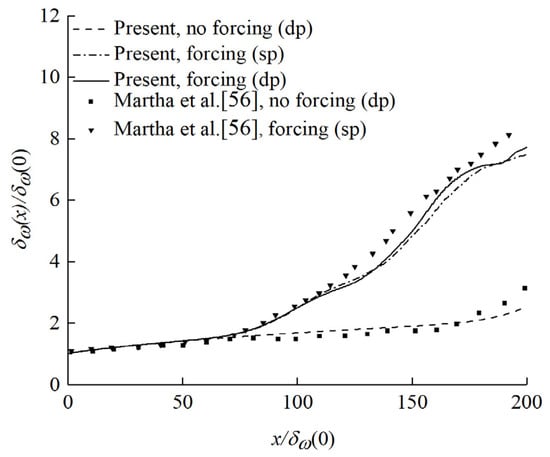
Figure 1.
Vorticity thickness growth rate of turbulent mixing layer in the original case.

Table 1.
Comparison of the results of the original case with the results of previous experiments and computations.
In order to study the suitability of the time step, a new time step computational case is carried out. The new time step size of 5 × 10⁻⁸ s is half of the original time step size of 1 × 10⁻⁷ s. The computational settings except for the time step are consistent with the original calculation. The computational results are shown in Table 2. It can be seen that the results of the new time step are very close to the original one, indicating that the time step of 1 × 10⁻⁷ s is suitable. Since the cross-wise size of the computational domain of the original case is too large, it can be optimized. The cross-wise range of the optimized computational domain is −25~25. Firstly, the corresponding optimized grid is generated according to the grid point distribution method of the original grid. Then, the x-direction is refined by 2 times, y-direction is refined by 2 times, x, y-direction is refined by 1.414 times, x and y-direction is refined by 2 times at the same time to generate four sets of refined grids. The computational settings of the new grid are consistent with those of the original one. The computational results are shown in Table 3. It can be seen that both x and y direction mesh have a great influence on the results. From 1.414-fold to 2-fold, the results converge gradually. Especially, the Reynolds stress in the downstream direction is very close to the previous DNS results.
Table 2.
Comparison of different time step computational results with previous DNS results.
Table 3.
Comparison of different grid resolution results with previous DNS results.
In order to further verify the above 2D computations, 3D studies are also conducted in this paper. The 3D computational domain extends from 0 to 350 in the streamwise x-direction, from −25 to 25 in the crosswise y-direction and from 0 to 10 in the spanwise z-direction. The grid points in the x, y and z directions are 1151, 145 and 51, respectively. The total grid points are of about 8 million (it takes about 50,000 CPU hours to finish the computation of 12 flow-through cycles). In this 3D grid, the minimum grid spacings in the x, y and z directions at the mixing layer centerline are 0.2, 0.165 and 0.2, respectively. The 3D grid also has a buffer zone, which is the same as that in the 2D grid. The spanwise boundaries in the 3D grid are treated as periodic. The rest of the boundary conditions and the numerical schemes are consistent with the 2D cases. To generate three-dimensional disturbance, in addition to adding random disturbance in the y-direction, we also set the velocity fluctuation algorithm of the spectral synthesizer [58] at the inlet. Table 4 demonstrates the 3D and 2D computational results. In this study, the 3D results have been found to be close to the 2D ones, which is consistent with the observations in Martha et al. [56].
Table 4.
Comparison of 2-D and 3-D computational results.
2.3. Dynamic Mode Decomposition Method
Here, the standard DMD algorithm is briefly introduced.
The n matrix snapshots obtained by experiment or numerical simulation can be written into a snapshot sequence matrix X and Y. the time interval between any two snapshots is △t.
It is assumed that the flow field xi+1 can be expressed by the linear mapping of flow field xi
where A is the system matrix of high dimensional flow field. If the dynamic system itself is nonlinear, then the process is a linear estimation process. According to the assumed linear mapping relation, matrix A can reflect the dynamic characteristics of the system. Due to the high dimension of A, it is necessary to calculate a from the data sequence by order reduction. Therefore
For matrix X, a matrix can be provided to replace the high dimensional matrix A, and the two matrices are similar. In order to find the orthogonal subspace of similarity transformation, the singular value decomposition of X is used to obtain the following:
The matrix Σ is a diagonal matrix, and the diagonal elements contain r singular values. In the process of singular value decomposition, only r main singular values can be retained and the remaining small singular values can be truncated, so as to reduce the numerical noise. The unitary matrices U and V obtained by SVD satisfy UHU = I and VHV = I. The calculation process of matrix can be regarded as the minimization problem of Frobenius norm
Then we can approximate A by
Since the matrix is a similar transformation of A, the matrix contains the main eigenvalues of A. The jth eigenvalue is λj and the eigenvector is wj. Then the jth DMD mode is defined as
The growth rate gj and frequency ωj corresponding to the jth mode are defined as follows:
When judging the stability, if the growth rate is positive, the corresponding mode is unstable; if the growth rate is negative, the corresponding mode is stable; if the growth rate is zero, the corresponding mode is periodic; if the eigenvalue falls within the unit circle, it means the stable mode, and vice versa.
The dynamic modes of the flow field can be extracted by the above-mentioned DMD method, and the evolution process of the flow field can be further estimated according to the reduced order matrix . By the singular value decomposition (15), the high-dimensional system xi can be mapped to the subspace zi
The governing equation of the reduced order system is obtained as follows:
Let W be a matrix whose column vector is the eigenvector wj, and let Ν be a diagonal matrix containing singular values, then the feature decomposition can be expressed as follows:
Therefore, the snapshot at any time can be estimated as
Each column of Φ is defined as a DMD mode,
According to Formula (15), there is
The modal amplitude α is defined as
where αi is the amplitude of the ith mode, which represents the contribution of the mode to the initial snapshot x1. For the standard DMD method, the DMD modes are sorted according to the amplitude. If Equations (26) and (27) are brought into Equation (25), the flow field can be predicted at any time
3. Results and Discussions
3.1. Characteristics of the Turbulent Mixing Layer
After verifying and confirming the large eddy simulation (LES) method of the turbulent mixing layer, this paper selects the grid which is refined twice in x and y directions to study the basic characteristics and disturbance effects of turbulent mixing layers. The results show that the grid number in x direction is 1151, the mesh number in buffer is 151, the stretch ratio is 1.04, the mesh number in y direction is 145, and the stretch ratio is 1.1. The time step is 1 × 10⁻⁷ s. Double precision is used in the calculation. In the study of basic characteristics, α in the inlet disturbance is obtained as 0.0045 (basic case); in the study of disturbance influence, α in inlet disturbance is obtained as 0, 0.0045, 0.045 and 0.45y.
3.1.1. Basic Characteristics of Turbulent Mixing Layer
Figure 2a shows the vorticity thickness growth rate of the basic case. It can be seen from the figure that the growth process of the turbulent mixing layer mainly presents two different stages. In the first stage, the flow is in laminar flow state, and the growth rate is relatively small, and the growth curve is approximately linear. The second stage flow is in turbulent state after transition, and the growth rate of turbulent state is significantly higher than that of the first stage, and the growth curve is also approximately linear.
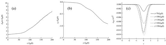
Figure 2.
(a) Vorticity thickness growth rate; (b) center line of mixing layer; (c) Reynolds shear stress curve.
The velocity center line of the turbulent mixing layer is obtained according to the following two equations:
where is the average streamwise velocity.
Figure 2b shows the velocity center line of the turbulent mixing layer, from which it can be seen that it has a significant bias to the low-speed side. Corresponding to the vorticity thickness growth curve in Figure 2a, there are two main sections in the velocity center line of Figure 2b, and the turning positions of the curves in the two graphs are the same, which indicates that the laminar/turbulent flow pattern also affects the degree of the velocity center line of the turbulent mixing layer to the low-speed side.
The Reynolds shear stress is dimensionless as follows:
The normal position is dimensionless as follows:
According to these two dimensionless quantities, the self-similarity of turbulent mixing layer can be observed. Figure 2c shows the curve. According to the curves of the five flow directions, the turbulent mixing layer is self-similar at about three-quarters of the flow direction in the physical computational domain. The Reynolds normal stress curves in x and y directions have similar phenomena, which are not provided here due to the length of paper.
Figure 3 shows the vorticity evolution contours in the physical domain of the last FTC (41,300~42,000 steps, with 100 steps interval). It can be seen that the turbulent mixing layer begins to lose stability at about one third of the flow direction in the physical domain, and then generates vortex rolling, falling, pairing and merging.
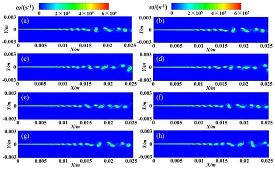
Figure 3.
Vorticity evolution in different instants.(a) 4.13ms; (b) 4.14ms; (c) 4.15ms; (d) 4.16ms; (e) 4.17ms; (f) 4.18ms; (g) 4.19ms; (h) 4.2ms.
3.1.2. Influence of Inlet Disturbance on Turbulent Mixing Layer
As mentioned above, in the study of disturbance influence, α in the inlet disturbance is taken as 0, 0.0045, 0.045 and 0.45 respectively. If α = 0.0045 corresponds to the reference disturbance, then α = 0 corresponds to no disturbance, α = 0.045 corresponds to 10 times disturbance, and α = 0.45 to 100 times disturbance.
Figure 4 shows the transient instantaneous vorticity contours of the last time of the 12 FTCs under different disturbances. It can be seen that the inlet disturbance significantly advances the flow direction of the mixing layer instability, and the influence on the instability increases with the increase of the inlet disturbance intensity.
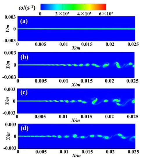
Figure 4.
Instantaneous vorticity contours with different forcing. (a) no forcing; (b) 1 forcing; (c) 10 forcing; (d) 100 forcing.
Figure 5a shows the vorticity thickness growth curve of turbulent mixing layer under different disturbances. It can be seen that with the increase of the disturbance, the turning position of the vorticity thickness growth curve is advanced, and the turning position of the vorticity thickness growth curve under 100 times disturbance is even ahead of the entrance. However, although the size of the disturbance significantly affects the turning position, it does not affect the growth rate of the turbulent mixing layer vorticity thickness after the turning point.
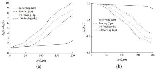
Figure 5.
(a) Vorticity thickness growth rates with different forcing; (b) center line of mixing layer with different forcing.
Figure 5b shows the variation curves of the velocity center line of the turbulent mixing layer under different disturbances. It can be seen that the greater the inlet disturbance, the greater the degree of the velocity center line deflecting to the low speed side. Under various disturbances, the turning position of velocity center line curve is always the same as that of vorticity thickness growth curve.
Figure 6 shows the Reynolds shear stress profile of turbulent mixing layer under different disturbances. It can be seen from Figure 6a that when there is no disturbance, there is a big difference between the peak shear Reynolds stress at and , and there is no self-similar state in the mixing layer; however, it can be seen from Figure 6b–d that when there is disturbance, the Reynolds shear stress profile downstream of the flow field is in close proximity, and the greater the disturbance is, the more forward the flow direction of self-similarity appears.
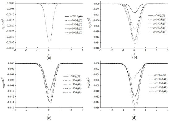
Figure 6.
Reynolds shear stress (a) no forcing; (b) 1 forcing; (c) 10 forcing; (d) 100 forcing.
3.2. Decomposition of Flow Field
In DMD analysis of flow field, 11~12 FTCs (35,000–42,000 steps) are sampled every 20 steps. A snapshot sample of 351 snapshots will therefore be obtained.
3.2.1. DMD Analysis of Basic Case
In this section, DMD analysis is carried out for x-direction velocity U, y-direction velocity V and vorticity ω.
Firstly, the x-direction velocity U is analyzed and as shown in Figure 7, the singular value arrangement, growth rate, frequency diagram, eigenvalue distribution diagram and part of the DMD modal contours (showing only the physical computational domain (0~0.0254 m)) is obtained.
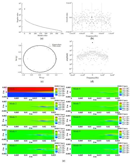
Figure 7.
DMD analysis of x-direction velocity U. (a) Singular value distribution; (b) modal growth rate versus frequency; (c) modal eigenvalues distribution; (d) modal amplitude versus frequency; (e) first 10 modes.
Figure 7a shows the order of singular values. The DMD modes are arranged in the order of singular values. As can be seen from Figure 7a, the first-order singular value is more than one order of magnitude higher than other singular values. In Table 5, the second column gives the singular values of the first 10 modes. The first- order singular value is utterly dominant, implying that after flow field decomposition, the first-order mode is the most important mode. From Figure 7a, it can be seen that the first mode is consistent with the average flow field.
Table 5.
Singular values and growth rates of the first 10 DMD modes.
Figure 7b shows the relationship between the modal growth rate and the frequency. The modal growth rate is symmetrical with respect to the frequency. The growth rate of the mode is equal to 0, which indicates that the mode does not shift. The mode growth rate is less than 0, which indicates that the mode is decaying and stable. When the mode growth rate is greater than 0, the mode is unstable. Figure 7b shows that most of the modal growth rates are below 0, which indicates that the whole system is stable.
Figure 7c shows the distribution of eigenvalues, where the horizontal axis is the real part of the modal eigenvalues and the vertical axis corresponds to the imaginary part. Most of the eigenvalues fall on and within the unit circle, and a few points fall outside the unit circle. Among them, mode 1 is located on the unit circle and the growth rate is 0, so mode 1 is static mode; the mode corresponding to the eigenvalue falling in the unit circle is stable mode; the mode corresponding to the eigenvalue falling outside the unit circle is unstable mode.
Figure 7d shows the relationship between modal amplitude and frequency. Modal amplitude is symmetrical with respect to frequency. The amplitude of the first mode is the largest, which indicates that the contribution of the first mode is the largest.
Figure 7e shows the contours of the first 10 modes, and Table 5 shows the singular values, growth rates and frequencies of the first 10 modes. It can be seen that except for mode 1, the other modes are paired. The singularities of the paired modes are close, the growth rates are equal, and the frequencies are opposite to each other. This is because the DMD modes are conjugate modes, which are essentially the same mode. The results show that the first 10 modal structures are strip shape in the flow direction, and the strip structure mainly exists in the middle and rear of the flow field, which is close to the vortex position of the mixing layer flow field, indicating that the structure is closely related to the formation of vortex. Figure 8 shows the DMD analysis results of velocity V in the y-direction. As can be seen from Figure 8a, there is no dominant singular value of velocity V. The singular values, growth rates and frequencies of the first 10 DMD modes are given in Table 6. From the growth rates and frequencies, it can be seen that the first 10 DMD modes are five pairs of conjugate modes, that is, the growth rates are equal and the frequencies are opposite to each other. The growth rates of the first six modes are all greater than 0, and they are all unstable modes. Figure 8b shows the relationship between the mode growth rate and frequency. The growth rate of the first mode is 1756, which is greater than 0, and the frequency is not 0. It indicates that it is unstable and not the primary mode of flow field. None of the modes meets the frequency and growth rate of 0 at the same time. Figure 8c shows the eigenvalues basically fall near the unit circle, but the first mode does not fall at (1,0) and none of the modes fall at (1,0). Figure 8d shows that the amplitude of the first mode is much smaller than that of the maximum mode.
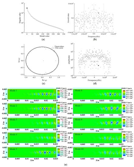
Figure 8.
DMD analysis of y-direction velocity Y. (a) Singular value distribution; (b) modal growth rate versus frequency; (c) modal eigenvalues distribution; (d) modal amplitude versus frequency (e) first 10 modes.
Table 6.
Singular values and growth rates of the first 10 DMD modes.
It can be seen from Figure 8e that the first 10 modes are identical, indicating that the corresponding modes are conjugate modes, and the flow field structure presents an alternating circular structure.
The results of DMD analysis of vorticity ω are shown in Figure 9. The DMD result of vorticity ω is similar to that of velocity U in x-direction. It is visible from Figure 9a that the dominant singular value of vorticity ω exists, and the first singular value is greater than the other singular values by more than one order of magnitude. It can be seen from Table 7 that except for the first mode, the others are conjugate modes. The growth rates of the first 10 modes are less than 0, indicating that they are stable modes. In Figure 9b, the first mode’s growth rate and frequency are both equal to zero. It shows that it is stable and the primary mode of flow field. Figure 9c shows that the eigenvalue basically falls near the unit circle, and the first mode falls at point (1, 0). Figure 9d shows the amplitude of the first mode is the largest. Figure 9e shows the first 10 modes, which is similar to the first 10 modes of velocity U. A slender and large-scale structure is shown by low-frequency modes 2–9.
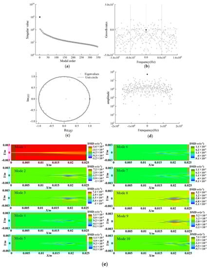
Figure 9.
DMD analysis of vorticity ω. (a) Singular value distribution; (b) modal growth rate versus frequency; (c) modal eigenvalues distribution; (d) modal amplitude versus frequency (e) first 10 modes.
Table 7.
Singular values and growth rates of the first 10 DMD modes.
3.2.2. DMD Analysis of Inlet Disturbance Characteristics
DMD analysis is carried out for different inlet disturbance conditions and the influence of disturbance amplitude is studied. The previous basic case is random disturbance condition α = 0.0045 (1 forcing). Here, two groups of random disturbance condition α = 0.045 (10 forcing), 0.45 (100 forcing) and one group of no forcing condition α = 0 are added. DMD analysis was carried out on the x-direction velocity U of the three groups of working conditions, and 351 snapshots were also sampled.
Figure 10a shows the order 2~350 singular value arrangement under four disturbance conditions. The first-order singular values of no forcing, forcing, 10 forcing and 100 forcing are 1,040,287.5, 1,045,597.5, 1,046,331.7 and 1,046,807.3, respectively. It can be seen that the larger the disturbance is, the larger the first-order singular value is. However, the difference between the three perturbed singular values is smaller than that between the perturbed and undisturbed singular values. As can be seen from Figure 10a, the first-order singular value is more than one order of magnitude larger than other singular values. The singular value of DMD with forcing is obviously larger than that without forcing. There is no significant difference in the singular values of the three disturbed conditions. It demonstrates that the composition of the flow field of the three kinds of conditions of disturbance is similar.
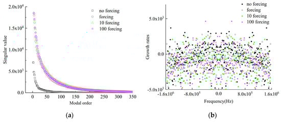
Figure 10.
DMD analysis of inlet disturbance characteristics. (a) Singular value distribution with different forcing; (b) modal growth rate versus frequency.
Figure 10b shows the relationship between the growth rate of the four disturbances and the frequency. Since the growth rate is symmetrical about the frequency, Figure 10b only shows the right half for easy observation. It can be seen that the growth rates of the four disturbances are mainly concentrated in the region of −5000~0, indicating that most of the modes are stable, and there is a point at the origin under each condition, and the corresponding dynamic mode at this point corresponds to the mean flow structure. In general, the larger the disturbance is, the farther away the points are from the origin. It shows that the nonlinear intensity of the disturbed flow field is directly related to the magnitude of the disturbance.
3.3. Reduced Order Reconstruction and Prediction of Flow Field
3.3.1. Reduced Order Reconstruction and Prediction of Basic Case
In this section, the flow field under basic case is reduced, and the first 150 orders are truncated (the sum of the first 150 singular values accounts for more than 90% of the total singular values). The reduced order reconstruction and prediction effect of DMD on the turbulent mixing layer flow field with strong nonlinearity are studied. The x-direction velocity U, y-direction velocity V and vorticity ω are reconstructed and predicted, respectively.
Figure 11a shows the comparison between the reconstructed contours and the instantaneous contours. The physical computational domain (0~0.0254 m) is compared. According to the vorticity contours, the flow field is divided into three regions: the region before instability, the rolling up region and the vortex interaction region. In the upstream of the flow field, there is no obvious fluid exchange and vortex structure. The vorticity concentrates on the shear line, and its width increases gradually along the flow direction. We call this region the pre-instability region. In the middle of the flow field (i.e., downstream of the region before instability), there is obvious material exchange between the upper and lower flow fields. An obvious single vortex (a series of vortex structures) can be observed from the vorticity contours. The distance between these vortex structures is approximately proportional to their own scale, and gradually increases along the flow direction. We call this region the roll up region. In the downstream of the flow field (that is, the downstream of the roll up region), the interaction between the vortices of the flow field occurs. We call this region the vortex interaction region.
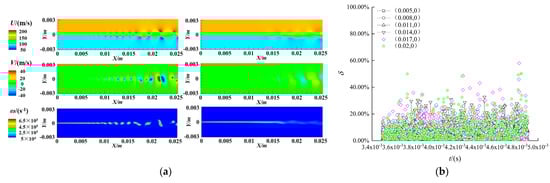
Figure 11.
150 order reconstruction and prediction of basic case. (a) Comparison of reconstruction contours (right) and instantaneous contours (left 42,000 steps) with forcing; (b) relative error.
It can be seen that in the basic case, whether it is velocity U, V or vorticity ω, the reconstruction effect of the flow field is poor, and only the region before instability (about 0~0.006 m region) can be reproduced. For the roll up region (about 0.006–0.015 m region) and vortex interaction region (about 0.015~0.0254 m region), the reconstruction effect of DMD is not good because of the strong nonlinearity of the region.
Six points (0.005,0), (0.008,0), (0.011,0), (0.014,0), (0.017,0) and (0.02,0) on the middle line of the physical computational domain are selected to further analyze the reconstruction and prediction of DMD.
Figure 11b is the reduced order reconstruction and prediction relative error diagrams of perturbed velocity U. Among them, 0.0035 s~0.0042 s is the time range within the sample, and 0.0042 s-0.0049 s is the predicted time range.
The relative error δ is defined as
where a is the reconstructed and predicted value of DMD and A is the actual value.
As can be seen more clearly from Figure 11b, the error of reconstruction segment is obviously less than that of prediction segment, most of the errors of reconstruction segment are less than 10%, a considerable part of the errors of prediction segment are more than 20%, and individual errors are more than 40%. The effect of velocity V and vorticity ω is similar, as such there is no additional illustration.
3.3.2. Influence of Dominant Mode Selection Method on Reduced Order Reconstruction and Prediction
After the flow field is decomposed, the selection of the dominant mode is the key step of flow field reduction reconstruction and prediction. At present, there is no specific method to select the dominant mode of the flow field after DMD decomposition. For different flow characteristics, the most suitable mode selection method may be different. In this section, four modal selection methods are compared: (1) according to the size of singular value; (2) according to the size of modal amplitude; (3) according to the size of modal energy [63]; (4) according to the size of the integral modal amplitude of sampling time [64], to investigate the mode selection method of the turbulent mixing layer suitable for this study.
Here, four methods are briefly introduced. The first and second methods are easier to understand. The expression of the third method is as follows:
where is the energy contained in the ith mode and is the flow velocity of each node in the ith mode.
In the fourth method, the integral modal amplitude is defined as [64]:
DMD analysis is carried out for the stochastically perturbed velocity U. Figure 12a shows the relationship between modal energy and frequency, from which it can be seen that high modal energy (greater than 0.7) is mainly concentrated near low frequency and high frequency, and the modal energy of middle frequency is almost about 0.7. The first three modes with the largest energy are shown in Figure 12a, which is named mode 1, mode A and mode B. The modal energy of mode 1 is the largest, and the frequency is 0 Hz. Mode 1 is the first-order mode arranged according to the eigenvalue, which also shows that the first-order mode is the most important mode. Mode A is the second-highest energy mode with a frequency of 1,567,540 Hz. Mode B is the third-highest energy mode with a frequency of 1,570,796 Hz. Modes A and B are high-frequency modes in the flow field. Figure 12b shows the relationship between the integral mode amplitude and frequency, and marks the three modes with the largest amplitude of integral mode which are also mode 1, mode A and mode B. Different from modal energy, modal B is larger than modal A. This shows that different methods extract the dominant mode differently. Compared with Figure 7d, we can see that the morphology has changed significantly. The integral amplitude of the first-order mode is still the largest, which shows once again that the first-order mode is the most important.
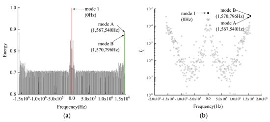
Figure 12.
Mode selection method 3 and 4. (a) Modal energy versus frequency; (b) integral modal amplitude versus frequency.
Figure 13 shows the contours of mode A and mode B. compared with modes 1~10 in Figure 7, it can be seen that the high-frequency modes present row upon row of small-scale structures. The low-frequency modes present large-scale structures.
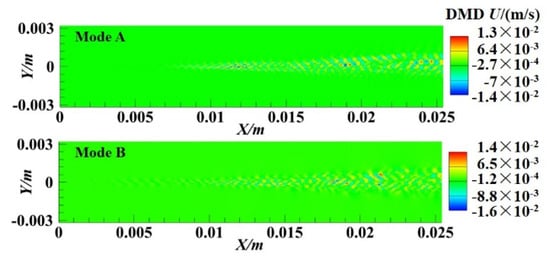
Figure 13.
Mode A and Mode B.
In order to ensure a certain accuracy and reduce the order of the flow field, four methods are used to select 150 modes to reconstruct and predict the velocity U flow field. The comparison results are shown in Figure 14 and Figure 15. It can be seen from Figure 14 that the reconstructed contours by methods 2 and 3 are close to the instantaneous contours and can reconstruct a smaller scale structure. The reconstructed contours by methods 1 and 4 are not ideal, only some large structures can be reconstructed, and the shape difference is large, which is very different from the instantaneous flow field. Figure 15 shows the comparison between the predicted contours and the instantaneous contours. It can be seen that the predicted results of all methods have some deviation. The prediction results of method 1 and method 3 are almost the same, both of which overestimate the flow field. The result of method 4 is still not optimal. In contrast, the prediction results of method 2 are closer to the transient flow field, which is better than the other three methods. Therefore, method 2 is selected as the modal selection method in this study.
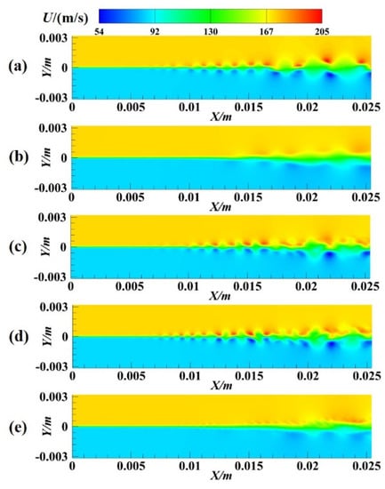
Figure 14.
(a) Instantaneous (42,000 steps) contours; (b) reconstructed contours by method 1; (c) reconstructed contours by method 2; (d) reconstructed contours by method 3; (e) reconstructed contours by method 4.
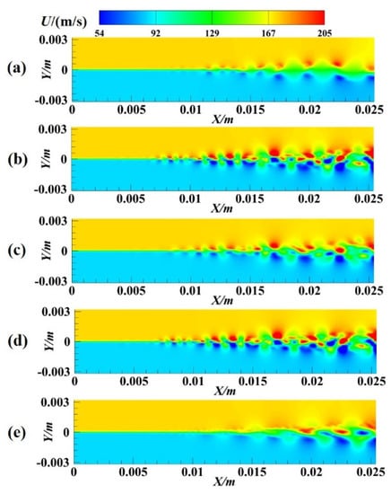
Figure 15.
(a) Instantaneous (49,000 steps) contours; (b) prediction contours by method 1; (c) prediction contours of method 2; (d) prediction contours by method 3; (e) prediction contours by method 4.
3.3.3. Influence of Inlet Disturbance on Reduced Order Reconstruction and Prediction
In this section, method 2 is used to select 150 modes for reconstruction and prediction to analyze the influence of disturbance existence (the difference between the undisturbed condition and the disturbed condition) and disturbance form (the difference between random disturbance and periodic disturbance).
Figure 16a shows the comparison between the undisturbed reconstructed contours (right side) and the instantaneous contours (left side). Figure 17a shows the comparison between the reconstructed contours (right side) and the instantaneous contours (left side). From top to bottom are U, V, and ω. Under the undisturbed condition, the flow field in the computational domain belongs to the region before instability, and the reconstructed contours are almost the same as the instantaneous contours. Compared with Figure 17a, it can be seen that the reconstruction effect of undisturbed DMD is better than that of perturbed DMD.
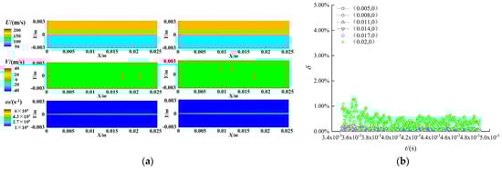
Figure 16.
150 order reconstruction and prediction of no forcing case. (a) Comparison of reconstruction (right) and instantaneous contours (left); (b) relative error.
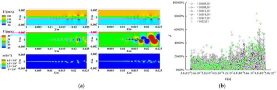
Figure 17.
150 order reconstruction and prediction of random forcing case. (a) Comparison of reconstruction (right) and instantaneous contours (left); (b) relative error.
As before, the same six points for reconstruction and prediction were selected. The relative error is shown in Figure 16b and Figure 17b. The fluctuation of each undisturbed point value with time is much smaller. In particular, the actual velocity of the points (0.005,0) and (0.008,0) near the entrance is almost unchanged. The relative error is within 1%. In general, the reconstruction and prediction of undisturbed DMD are better than that of perturbed DMD.
The influence of disturbance form is studied below. The disturbance conditions in the previous sections are all random disturbances. We added a group of periodic disturbance conditions for comparative study. The computational settings are consistent with that in Section 2. The sampling method is also consistent with random disturbance, and 351 snapshots are obtained. The periodic disturbance formula is as follows:
where α, ∆y0 consistent with Section 2.2.2, t is the time variable.
Figure 18a shows the comparison between the reconstructed contours of 150 modes selected by method 2 and the instantaneous contours. It is obvious that the reconstruction effect is ideal, and the reconstructed contours are almost the same as the instantaneous contours. The shape of the whole flow field, the size and the position of the vortex are almost the same. From the comparison of the instantaneous contours in Figure 17a and Figure 18a, it can be seen that the flow field under the condition of random disturbance develops faster than that under the condition of periodic disturbance. The results show that the flow field under the random disturbance condition consists of the pre-instability region, the rolling up region, the vortex interaction region, and the rolling up the position of the vortex is about 0.007 m in the x-direction. However, there is no obvious vortex interaction zone in the flow field under the condition of periodic disturbance, and the vortex curling position is about 0.017 m in the x-direction.
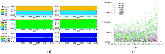
Figure 18.
150 order reconstruction and prediction of periodical forcing case. (a) Comparison of reconstruction (right) and instantaneous contours (left); (b) relative error.
Similarly, the six selected points are reconstructed and predicted, and the relative error is shown in Figure 18b. Except for the point (0.02, 0), the error of other points is less than 5%. Compared with the results of random disturbance in Figure 17, it can be seen that DMD has poor reconstruction and prediction effect for highly nonlinear and aperiodic conditions, but good reconstruction and prediction effect for periodic disturbance conditions.
4. Conclusions
In the present paper, large eddy simulation (LES) and dynamic mode decomposition (DMD) were used to study turbulent mixing layers. The results allow for the following conclusions to be drawn:
(1) The LES method used in this paper can accurately calculate the vorticity thickness growth rate of the turbulent mixing layer, and the peak values of each component of Reynolds stress at several streamwise locations are close to the results of DNS in literature, indicating that the present LES provides accurate big data for DMD.
(2) For the velocity in x-direction, the first-order mode is the dominant mode of the flow field, which represents the average flow field; the low-frequency mode presents a strip-shaped large-scale structure, and the high-frequency mode presents a small-scale structure, which indicates that the small-scale vortex formation in the flow field is mainly related to the high-frequency mode. For the velocity in y-direction, the first-order mode is unstable, which cannot represent the average flow field; there is no mode in which frequency and growth rate are both zero, which indicates that the flow field of velocity in y-direction is more complex than that of velocity in x-direction.
(3) The dominant-mode selection criterion based on mode amplitude is more suitable for turbulent mixing layer flow compared with the other three criteria based on singular value, modal energy and integral modal amplitude.
(4) The standard DMD method reconstructs and predicts the periodically-perturbed mixing layer well. In contrast, for the mixing layer with random disturbance, the standard DMD method could only accurately reconstruct and predict the region before instability happens but is not qualified in the regions after that as nonlinearity is stronger, which implies that improved dynamic mode decomposition methods need to be utilized or developed for the future dynamic mode decomposition of turbulent mixing layers.
Author Contributions
Investigation, computation, visualization, formal analysis, and writing—original draft, Y.C.; conceptualization, methodology, investigation, formal analysis, writing—original draft, writing—review, and supervision, Q.C. All authors have read and agreed to the published version of the manuscript.
Funding
This work was supported by the National Natural Science Foundation of China (Grant No. 91741102), the Shenzhen Fundamental Research Program (Grant No. JCYJ20190807160413162) and the Fundamental Research Funds for the Central Universities (Grant No. 19lgzd15).
Institutional Review Board Statement
Not applicable.
Informed Consent Statement
Not applicable.
Data Availability Statement
Not applicable.
Acknowledgments
The authors would like to express their thanks for the support of the National Natural Science Foundation of China (Grant No. 91741102), the Shenzhen Fundamental Research Program (Grant No. JCYJ20190807160413162) and the Fundamental Research Funds for the Central Universities (Grant No. 19lgzd15).
Conflicts of Interest
The authors declare no conflict of interest.
References
- Ho, C.M.; Huerre, P. Perturbed free shear layers. Annu. Rev. Fluid Mech. 1984, 16, 365–424. [Google Scholar] [CrossRef]
- Dimotakis, P.E. Turbulent mixing. Annu. Rev. Fluid Mech. 2005, 37, 329–356. [Google Scholar] [CrossRef]
- Livescu, D. Turbulence with large thermal and compositional density variations. Annu. Rev. Fluid Mech. 2020, 52, 309–341. [Google Scholar] [CrossRef]
- McMullan, W.A.; Garrett, S.J. Initial condition effects on large scale structure in numerical simulations of plane mixing layers. Phys. Fluids 2016, 28, 015111. [Google Scholar] [CrossRef]
- Tan, J.; Li, H.; Noack, B.R. On the cavity-actuated supersonic mixing layer downstream a thick splitter plate. Phys. Fluids 2020, 32, 096102. [Google Scholar] [CrossRef]
- Zhang, D.; Tan, J.; Yao, X. Direct numerical simulation of spatially developing highly compressible mixing layer: Structural evolution and turbulent statistics. Phys. Fluids 2019, 31, 036102. [Google Scholar] [CrossRef]
- Baltzer, J.R.; Livescu, D. Variable-density effects in incompressible non-buoyant shear-driven turbulent mixing layers. J. Fluid Mech. 2020, 900, A16. [Google Scholar] [CrossRef]
- Ren, Z.; Wang, B.; Zheng, L. Numerical analysis on interactions of vortex, shock wave, and exothermal reaction in a supersonic planar shear layer laden with droplets. Phys. Fluids 2018, 30, 036101. [Google Scholar] [CrossRef]
- Chen, Q.; Wang, B. The spatial growth of supersonic reacting mixing layers: Effects of combustion mode. Aerosp. Sci. Technol. 2021, 116, 106888. [Google Scholar] [CrossRef]
- Brunton, S.L.; Noack, B.R.; Koumoutsakos, P. Machine learning for fluid mechanics. Annu. Rev. Fluid Mech. 2020, 52, 477–508. [Google Scholar] [CrossRef]
- Berkooz, G.; Holmes, A.P.; Lumley, J.L. The proper orthogonal decomposition in the analysis of turbulent flows. Annu. Rev. Fluid Mech. 2003, 25, 539–575. [Google Scholar] [CrossRef]
- Schmid, P.J. Dynamic mode decomposition of numerical and experimental data. J. Fluid Mech. 2010, 656, 5–28. [Google Scholar] [CrossRef]
- Duke, D.; Soria, J.; Honnery, D. An error analysis of the dynamic mode decomposition. Exp. Fluids 2012, 52, 529–542. [Google Scholar] [CrossRef]
- Bagheri, S. Effects of weak noise on oscillating flows: Linking quality factor, Floquet modes, and Koopman spectrum. Phys. Fluids 2014, 26, 094104. [Google Scholar] [CrossRef]
- Pan, C.; Xue, D.; Wang, J. On the accuracy of dynamic mode decomposition in estimating instability of wave packet. Exp. Fluids 2015, 56, 164. [Google Scholar] [CrossRef]
- Chen, K.K.; Tu, J.H.; Rowley, C.W. Variants of Dynamic Mode Decomposition: Boundary Condition, Koopman, and Fourier Analyses. J. Nonlinear Sci. 2012, 22, 887–915. [Google Scholar] [CrossRef]
- Jovanovic, M.R.; Schmid, P.J.; Nichols, J.W. Sparsity-promoting dynamic mode decomposition. Phys. Fluids 2014, 26, 024103. [Google Scholar] [CrossRef]
- Hemati, M.S.; Williams, M.O.; Rowley, C.W. Dynamic mode decomposition for large and streaming datasets. Phys. Fluids 2014, 26, 111701. [Google Scholar] [CrossRef]
- Hemati, M.S.; Rowley, C.W.; Deem, E.A.; Cattafesta, L.N. De-biasing the dynamic mode decomposition for applied Koopman spectral analysis of noisy datasets. Theor. Comput. Fluid Dyn. 2017, 31, 349–368. [Google Scholar] [CrossRef]
- Noack, B.R.; Stankiewicz, W.; Morzynski, M.; Schmid, P.J. Recursive dynamic mode decomposition of transient and post-transient wake flows. J. Fluid Mech. 2016, 809, 843–872. [Google Scholar] [CrossRef]
- Sayadi, T.; Schmid, P.J.; Richecoeur, F.; Durox, D. Parametrized data-driven decomposition for bifurcation analysis, with application to thermo-acoustically unstable systems. Phy. Fluids 2015, 27, 037102. [Google Scholar] [CrossRef]
- Kutz, J.N.; Fu, X.; Brunton, S.L. Multiresolution Dynamic Mode Decomposition. SIAM J. Appl. Dyn. Syst. 2016, 15, 713–735. [Google Scholar] [CrossRef]
- Gueniat, F.; Mathelin, L.; Pastur, L.R. A dynamic mode decomposition approach for large and arbitrarily sampled systems. Phys. Fluids 2015, 27, 025113. [Google Scholar] [CrossRef]
- Williams, M.O.; Kevrekidis, I.G.; Rowley, C.W. A Data-Driven Approximation of the Koopman Operator: Extending Dynamic Mode Decomposition. J. Nonlinear Sci. 2015, 25, 1307–1346. [Google Scholar] [CrossRef]
- Pirozzoli, S.; Bernardini, M.; Marie, S.; Grasso, F. Early evolution of the compressible mixing layer issued from two turbulent streams. J. Fluid Mech. 2015, 777, 196–218. [Google Scholar] [CrossRef][Green Version]
- Liu, Y.; Dong, M.; Fu, B.; Qiang, L.; Zhang, C. Direct numerical simulation of fine flow structures of subsonic-supersonic mixing layer. Aerosp. Sci. Technol. 2019, 95, 105431. [Google Scholar]
- Arote, A.; Bade, M.; Banerjee, J. On coherent structures of spatially oscillating planar liquid jet developing in a quiescent atmosphere. Phys. Fluids 2020, 32, 082111. [Google Scholar] [CrossRef]
- Ye, C.-C.; Zhang, P.-J.-Y.; Wan, Z.-H.; Sun, D.-J.; Lu, X.-Y. Numerical investigation of the bevelled effects on shock structure and screech noise in planar supersonic jets. Phys. Fluids 2020, 32, 086103. [Google Scholar] [CrossRef]
- Rao, S.M.V.; Karthick, S.K.; Anand, A. Elliptic supersonic jet morphology manipulation using sharp-tipped lobes. Phys. Fluids 2020, 32, 086107. [Google Scholar] [CrossRef]
- Ayyappan, D.; Kumar, A.S.; Vaidyanathan, A.; Nandakumar, K. Study on instability of circular liquid jets at subcritical to supercritical conditions using dynamic mode decomposition. Phys. Fluids 2020, 32, 014107. [Google Scholar] [CrossRef]
- Li, X.-R.; Zhang, X.-W.; Hao, P.-F.; He, F. Acoustic feedback loops for screech tones of underexpanded free round jets at different modes. J. Fluid Mech. 2020, 902, A17. [Google Scholar] [CrossRef]
- Montagnani, D.; Auteri, F. Non-modal analysis of coaxial jets. J. Fluid Mech. 2019, 872, 665–696. [Google Scholar] [CrossRef]
- Alenius, E. Mode switching in a thick orifice jet, an LES and dynamic mode decomposition approach. Comput. Fluids 2014, 90, 101–112. [Google Scholar] [CrossRef]
- Kalghatgi, P.; Acharya, S. Modal Analysis of Inclined Film Cooling Jet Flow. J. Turbomach. 2014, 136, 081007. [Google Scholar] [CrossRef]
- Liu, Q.; Luo, Z.; Deng, X.; Wang, L.; Zhou, Y. Numerical investigation on flow field characteristics of dual synthetic cold/hot jets using POD and DMD methods. Chin. J. Aeronaut. 2020, 33, 73–87. [Google Scholar] [CrossRef]
- De, A.K.; Sarkar, S. Three-dimensional wake dynamics behind a tapered cylinder with large taper ratio. Phys. Fluids 2020, 32, 063604. [Google Scholar] [CrossRef]
- Yin, G.; Ong, M.C. On the wake flow behind a sphere in a pipe flow at low Reynolds numbers. Phys. Fluids 2020, 32, 103605. [Google Scholar] [CrossRef]
- Kumar, P.; Tiwari, S. Effect of incoming shear on unsteady wake in flow past surface mounted polygonal prism. Phys. Fluids 2019, 31, 113607. [Google Scholar] [CrossRef]
- Parkin, D.J.; Thompson, M.C.; Sheridan, J. Numerical analysis of bluff body wakes under periodic open-loop control. J. Fluid Mech. 2014, 739, 94–123. [Google Scholar] [CrossRef]
- Loosen, S.; Meinke, M.; Schroeder, W. Numerical Investigation of Jet-Wake Interaction for a Dual-Bell Nozzle. Flow Turbul. Combust. 2020, 104, 553–578. [Google Scholar] [CrossRef]
- Alessandri, A.; Bagnerini, P.; Gaggero, M.; Lengani, D.; Simoni, D. Dynamic mode decomposition for the inspection of three-regime separated transitional boundary layers using a least squares method. Phys. Fluids 2019, 31, 044103. [Google Scholar] [CrossRef]
- Tong, F.; Li, X.; Duan, Y.; Yu, C. Direct numerical simulation of supersonic turbulent boundary layer subjected to a curved compression ramp. Phys. Fluids 2017, 29, 125101. [Google Scholar] [CrossRef]
- Priebe, S.; Tu, J.H.; Rowley, C.W.; Martin, M.P. Low-frequency dynamics in a shock-induced separated flow. J. Fluid Mech. 2016, 807, 441–477. [Google Scholar] [CrossRef]
- He, G.; Wang, J.; Pan, C. Initial growth of a disturbance in a boundary layer influenced by a circular cylinder wake. J. Fluid Mech. 2013, 718, 116–130. [Google Scholar] [CrossRef]
- Nichols, J.W.; Larsson, J.; Bernardini, M.; Pirozzoli, S. Stability and modal analysis of shock/boundary layer interactions. Theor. Comp. Fluid Dyn. 2017, 31, 33–50. [Google Scholar] [CrossRef]
- Waindim, M.; Agostini, L.; Larcheveque, L.; Adler, M.; Gaitonde, D.V. Dynamics of separation bubble dilation and collapse in shock wave/turbulent boundary layer interactions. Shock Waves 2020, 30, 63–75. [Google Scholar] [CrossRef]
- Garicano-Mena, J.; Li, B.; Ferrer, E.; Valero, E. A composite dynamic mode decomposition analysis of turbulent channel flows. Phys. Fluids 2019, 31, 115102. [Google Scholar] [CrossRef]
- Wang, P.; Deng, Y.; Liu, Y. Vortex dynamics during acoustic-mode transition in channel branches. Phys. Fluids 2019, 31, 085109. [Google Scholar]
- Le Clainche, S.; Izbassarov, D.; Rosti, M.; Brandt, L.; Tammisola, O. Coherent structures in the turbulent channel flow of an elastoviscoplastic fluid. J. Fluid Mech. 2020, 888, A5. [Google Scholar] [CrossRef]
- Gomez, F.; Blackburn, H.M.; Rudman, M.; McKeon, B.J.; Luhar, M.; Moarref, R.; Sharma, A.S. On the origin of frequency sparsity in direct numerical simulations of turbulent pipe flow. Phys. Fluids 2014, 26, 101703. [Google Scholar] [CrossRef]
- Gomez, F.; Blackburn, H.M.; Rudman, M.; Sharma, A.S.; McKeon, B.J. Streamwise-varying steady transpiration control in turbulent pipe flow. J. Fluid Mech. 2016, 796, 588–616. [Google Scholar] [CrossRef]
- Srinivasan, G.; Mahapatra, S.; Sinhamahapatra, K.P.; Ghosh, S. Dynamic mode decomposition of supersonic turbulent pipe flow with and without shock train. J. Turbul. 2020, 21, 1–16. [Google Scholar] [CrossRef]
- Kou, J.; Zhang, W. Dynamic mode decomposition with exogenous input for data-driven modeling of unsteady flows. Phys. Fluids 2019, 31, 057106. [Google Scholar]
- Naderi, M.H.; Eivazi, H.; Esfahanian, V. New method for dynamic mode decomposition of flows over moving structures based on machine learning (hybrid dynamic mode decomposition). Phys. Fluids 2019, 31, 127102. [Google Scholar] [CrossRef]
- Nair, A.G.; Strom, B.; Brunton, B.W.; Brunton, S.L. Phase-consistent dynamic mode decomposition from multiple overlapping spatial domains. Phys. Rev. Fluids 2020, 5, 074702. [Google Scholar] [CrossRef]
- Martha, C.S.; Blaisdell, G.A.; Lyrintzis, A.S. Large eddy simulations of 2-D and 3-D spatially developing mixing layers. Aerosp. Sci. Technol. 2013, 31, 59–72. [Google Scholar] [CrossRef]
- Uzun, A. 3-D large Eddy Simulation for Jet Aero Acoustics. Ph.D. Thesis, School of Aeronautics and Astronautics, Purdue University, West Lafayette, IN, USA, 2003. [Google Scholar]
- Fluent, A. Ansys Fluent User’s Guide; ANSYS Inc.: Canonsburg, PA, USA, 2021; Volume 15317. [Google Scholar]
- Wygnanski, I.; Fiedler, H.E. The two dimensional mixing region. J. Fluid Mech. 1970, 41, 327–361. [Google Scholar] [CrossRef]
- Jones, B.G.; Spencer, B.W. Statistical Investigation of Pressure and Velocity Fields in the Turbulent Two-Stream Mixing Layer; AIAA Paper: Palo Alto, CA, USA, 1971. [Google Scholar]
- Bell, J.H.; Mehta, R.D. Development of a two-stream mixing layer from tripped and untripped boundary layers. AIAA J. 1990, 28, 2034–2042. [Google Scholar] [CrossRef]
- Stanley, S.; Sarkar, S. Simulations of spatially developing two-dimensional shear layers and jets. Theor. Comput. Fluid Dyn. 1997, 9, 121–147. [Google Scholar] [CrossRef]
- Rowley, C.W.; Mezic, I.; Bagheri, S.; Schlatter, P.; Henningson, D.S. Spectral analysis of nonlinear flows. J. Fluid Mech. 2009, 641, 115–127. [Google Scholar] [CrossRef]
- Kou, J.; Zhang, W. An improved criterion to select dominant modes from dynamic mode decomposition. Eur. J. Mech.-B/Fluids 2017, 62, 109–129. [Google Scholar] [CrossRef]


Publisher’s Note: MDPI stays neutral with regard to jurisdictional claims in published maps and institutional affiliations. |
© 2021 by the authors. Licensee MDPI, Basel, Switzerland. This article is an open access article distributed under the terms and conditions of the Creative Commons Attribution (CC BY) license (https://creativecommons.org/licenses/by/4.0/).