Abstract
The use of the tapered Gutenberg-Richter distribution in earthquake source models is rapidly increasing, allowing overcoming the definition of a hard threshold for the maximum magnitude. Here, we expand the classical maximum likelihood estimation method for estimating the parameters of the tapered Gutenberg-Richter distribution, allowing the use of a variable through-time magnitude of completeness. Adopting a well-established technique based on asymptotic theory, we also estimate the uncertainties relative to the parameters. Differently from other estimation methods for catalogs with a variable completeness, available for example for the classical truncated Gutenberg-Richter distribution, our approach does not need the assumption on the distribution of the number of events (usually the Poisson distribution). We test the methodology checking the consistency of parameter estimations with synthetic catalogs generated with multiple completeness levels. Then, we analyze the Atlantic ridge seismicity, using the global centroid moment tensor catalog, finding that our method allows better constraining distribution parameters, allowing the use more data than estimations based on a single completeness level. This leads to a sharp decrease in the uncertainties associated with the parameter estimation, when compared with existing methods based on a single time-independent magnitude of completeness. This also allows analyzing subsets of events, to deepen data analysis. For example, separating normal and strike-slip events, we found that they have significantly different but well-constrained corner magnitudes. Instead, without distinguishing for focal mechanism and considering all the events in the catalog, we obtain an intermediate value that is relatively less constrained from data, with an open confidence region.
1. Introduction
The Gutenberg-Richter law [1] is the most widely applied magnitude frequency distribution for earthquakes. If we look only to the distribution of the magnitudes, independently from the rate of events, this law corresponds to an exponential distribution [2]. In this case, it depends on only one parameter (the so-called b-value), controlling the slope of the distribution, and does not have an upper bound for the magnitude. In order to have a more physical behavior for the right tail of the magnitude distribution, two other formulations of this law are usually applied: the truncated and the tapered Gutenberg-Richter distributions [3]. The truncated version applies a hard bound to the tail, i.e., a maximum magnitude (Mmax). Instead, the tapered version applies a soft bound, i.e., a corner magnitude (): the probability of an earthquake bigger than the corner magnitude decreases very rapidly asymptotically reaching zero (see Figure 1).
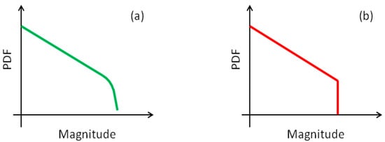
Figure 1.
Probability density functions of the tapered (a) and truncated (b) Gutenberg-Richter distributions, in a log10 Y-axis scale.
For these two formulations of the Gutenberg-Richter distribution, we need an extra parameter to be estimated: the maximum and the corner magnitude for the truncated and the tapered distributions, respectively. Regarding the estimation of the maximum magnitude, Zöller and Holschneider summarized very well the state of the art: “the earthquake history in a fault zone tells us almost nothing about Mmax” [4]. This and other papers [5,6,7] clearly show that a maximum likelihood estimation (MLE) of Mmax is not applicable, as the MLE is equal to the maximum observed magnitude and this may be problematic, considering the relatively short observation time as compared with mean recurrence times of large magnitude events. Conversely, the corner magnitude can be properly estimated if a sufficiently large amount of data is available [8]. The tapered Gutenberg-Richter distribution, also called tapered Pareto distribution or “Kagan distribution” by some statistical seismologists, was deeply investigated primarily by Kagan and Schoenberg [8], and then by Kagan [3], Schoenberg and Patel [9], and Geist and Parsons [7]. All these works use seismic catalogs with a single magnitude of completeness. These methods do not need any assumption on the distribution of the number of events. However, the size of the catalog can largely be expanded by adopting multiple levels of completeness, with a completeness magnitude that decreases in time, as the quality and quantity of the available instrumentation improve (Figure 2). This allows including in the estimation both the large number of relatively small events recorded by modern monitoring networks, and the larger events that occurred in the past, possibly also from pre-instrumental times [10].
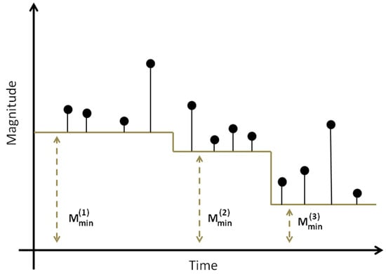
Figure 2.
Time vs. magnitude plot for a catalog with a variable magnitude of completeness (). The grey line represents the completeness, black dots the seismic events.
Existing methods [10,11,12] that deal with this problem need an assumption regarding the distribution through the time of the events. The distribution usually assumed is the Poisson distribution. This assumption is not always correct for the events in seismic catalogs, in particular if the magnitude of completeness of the catalog is lower than Mw 6.5 [13], forcing the application of declustering algorithms. On the other hand, declustering decreases the number of usable data and may introduce important biases in parameter estimations [14], which may even depend on the declustering algorithm selected.
This paper aims to develop a method to perform the parameters’ estimation for catalog with a variable magnitude of completeness (see Figure 2), without making any assumption on the distribution of the number of events. Thus, such a method can take the pros of both the previously described approaches, avoiding the cons relative to the single level of completeness and the Poisson assumption, allowing to use more data in the data estimation.
In the following, we first introduce the method and then we apply it to the Atlantic ridge seismicity. This region is characterized by shallow seismicity with a prevalence of normal/strike-slip mechanisms. The statistics of seismicity for oceanic spreading ridges was already studied in Bird et al. [15] and Bird and Kagan [16], which estimated for these zones a corner magnitude lower than other parts of the world (). Here, focusing on the Atlantic ridge with a longer catalog and our newly developed methodology, we improve the estimation of the parameters of the tapered Gutenberg-Richter distribution exploiting the potentiality of the newly developed method.
2. Methods
2.1. Maximum Likelihood Estimation of the Parameters
The Gutenberg-Richter distribution and all its derivations were originally developed using magnitudes. If we use seismic moments () instead of magnitudes, the Gutenberg-Richter distributions (unbounded/truncated/tapered) correspond to the Pareto distributions defined in Kagan [3], with slope parameter equal to 2/3 the b-value.
The probability density function of the tapered distribution is [3]:
where is the seismic moment of completeness of the catalog, is the parameter controlling the slope of the distribution, and is the corner moment that controls the tail of the distribution. We stress that it is always possible to pass from the seismic moment to the magnitude distribution (here, we adopt the relationship defined in Kanamori [17]. In this case the corner moment is called “corner magnitude” (), and the seismic moment of completeness corresponds to the magnitude of completeness.
If we have a seismic moment of completeness that varies with time (, Figure 2), we can easily rewrite Equation (1) with:
This relationship allows referring each observation to the completeness that holds at the time of its occurrence: in this time frame, indeed, Equation (2) describes the statistical distribution that holds.
Being both the parameters of the distribution ( and ) in common to all these distributions ( is a parameter related to the seismic catalog, estimated independently), their likelihood holds for all such distributions. Thus, if we have a seismic catalog with earthquakes with moments , the log-likelihood of the tapered Pareto distribution becomes:
In Equation (3) the probability density function depends on the seismic moment of completeness relative to the i-th earthquake. In Figure 3 we summarize the scheme of our methodology, applied to completeness thresholds relative to Figure 2: in this case the log-likelihood of Equation (3) is obtained by summing up the log-likelihoods relative to the three different thresholds of completeness. Notably, if the seismic moment of completeness is the same for all the events, Equation (3) becomes the classical log-likelihood for the tapered Pareto distribution [3].
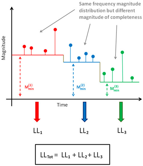
Figure 3.
Graphical representation of the log-likelihood computation scheme proposed in this paper in the case of three different magnitudes of completeness thresholds.
To maximize the likelihood of observations, and evaluate the maximum likelihood estimation (MLE) of the parameters and , we adopt a brute-force approach, that is, we evaluated the log-likelihood for many potential combinations of the parameters, covering the entire parameter space [12], This allows obtain the complete description of the log-likelihood function: the maximum of the function () is, by definition, the MLE of the parameters. Moreover, this approach allows evaluating also the shape of the log-likelihood function, which is particularly useful to assess the uncertainty associated with the parameters’ estimation, as it will be shown in the next section.
We stress the simplicity of our approach: to move from Equation (1) to Equation (2) we only need to substitute with , i.e., using the time-variable seismic moment of completeness instead of the fixed one. As the parameters of the distribution that we want to evaluate are in common to all periods, we can simply stack their likelihoods, passing to Equation (3). Noteworthy, this is based on the same principle exploited in Vere-Jones et al. [18], who used a standard log-likelihood function for a tapered Pareto distribution with one or more parameters that change with times (Vere-Jones et al. [18], Equation (19)), as also in that case, this is possible because each distribution holds at the time of the observation and the different likelihoods can be stacked by summing them (Figure 3).
To check the robustness of this approach, we test its performance by estimating the distribution parameters from synthetic catalogs, for which such parameters are known. To this end, we simulate, using the Taroni and Selva [11] toolbox (based on the Vere-Jones et al. [18] method), thousands of synthetic catalogs with different input parameters (, , and magnitude of completeness), obtaining a good agreement between the MLE of the parameters and the input parameters, as expected. The results are shown in Table 1. The goodness of the agreement should be evaluated based on the estimated uncertainty on the parameters. Thus, the results of this comparison are discussed in the next section.

Table 1.
Input and estimated and
relative confidence region for thousands of simulated synthetic catalogs.
2.2. Estimation of the Uncertainties
To evaluate the uncertainties relative to the parameters’ estimation, we use a widely applied method [3,7,8,16,19] based on asymptotic theory [20], sometimes called profile-likelihood confidence region estimation [21]. It states that, if we want to estimate the confidence region of the parameters (in our case, of the tapered Gutenberg-Richter), we have to “cut” the log-likelihood function at a fixed threshold, and then look at the contour plot of this cut. Different thresholds correspond to different confidence intervals. For example, to obtain a 95% confidence region, we have to look at the threshold, where is the maximum of the log-likelihood [8]. Hereinafter, the confidence region that describes the uncertainties on the parameters’ estimation will be represented by the contour plot of the selected threshold (see Figure 4 for an illustrative example).
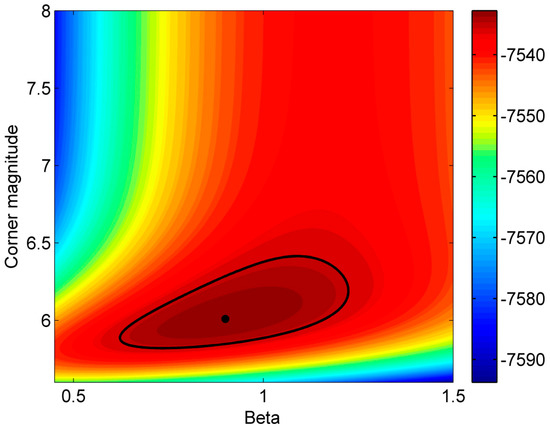
Figure 4.
Contour plot of the bivariate log-likelihood function for the parameters of the Tapered Gutenberg-Richter distribution; different colors represent the different log-likelihood values, according to the color bar on the left; the black curve represents the 95% confidence region, and the black dot represents the maximum likelihood estimation MLE.
This procedure is adopted to evaluate the goodness of the agreement between input and estimated parameters for the thousands of synthetic catalogs discussed in the previous paragraph. In particular, we verify that the input parameters are enclosed in the 95% confidence region for the estimated parameters about 95% of the simulations, obtaining a very good agreement. The results are shown in Table 1.
3. Data
As reference seismic catalog, we use the global centroid moment tensor (CMT) catalog [22,23] of shallow seismicity (depth ≤ 50 km) from 1980 to 2019. We do not decluster the catalog, to better exploit the potentiality of our method that does not assume any temporal distribution for earthquakes. As already commented above, this allows using more data and avoiding the introduction of the biases induced by declustering on the estimation [14,24]. We selected the events in the Atlantic ridge approximately in the latitude range −60°:60° (see Figure 5a).
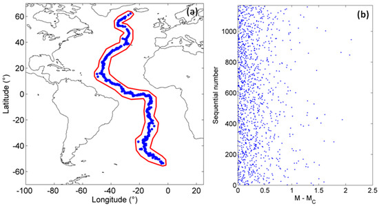
Figure 5.
Panel (a): events in the Atlantic ridge selected from the CMT catalog (blue dots) inside the red polygon; panel (b): difference between the magnitude of events and the relative completeness (M − MC) vs. the sequential number of events.
Regarding the magnitude of completeness, we use 5.5 from 1980 and 5.0 from 2004, the ones suggested by the authors of the catalog ([23], see Figure 6). We then carefully test this choice of completeness: as suggested by Marzocchi et al. [25], if the catalog is complete the magnitudes must follow an exponential distribution, and the exponentiality of the magnitudes can be tested through the Lilliefors [26] test. To apply this test with multiple completeness levels, we can build a vector of variables by subtracting to each magnitude the corresponding magnitude of completeness (), and test the exponentiality of this dataset [27]. The hypothesis of exponential distribution cannot be rejected at any confidence levels, as we obtain a very large p-value (0.50). This demonstrates the robustness of the chosen magnitudes of completeness. A further check is also performed in Figure 5b by plotting the vs. the sequential number of events: as suggested by Zhuang et al. [28], a homogeneous pattern near the Y-axis (as it is possible to see in Figure 1b) suggests the correct selection of completeness values for the catalog. The final catalog contains 1168 events.
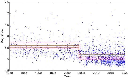
Figure 6.
Time vs. magnitude plot; blue dots represent seismic events, red lines the magnitude of completeness thresholds; the solid red line represents the reference level (Mw 5.5 from 1980 and Mw 5.0 from 2004), dashed red lines represent the conservative levels (+0.1 and +0.2 on the reference level).
4. Results
We estimate the corner magnitude and the of the tapered Pareto distribution both for the whole catalog and for two sub-catalogs: the one containing only normal events and the one containing only the strike-slip events. To select the event in the sub-catalogs, we use the classical Aki-Richards convention for rake: we consider as normal the events with the rake of both nodal planes of the CMT catalog in the range from −45° to −135°, and as strike-slip the events with the rake of both nodal planes of the CMT catalog in the range from −45° to 45° or 135° to 180° or −180° to −135°. When the two nodal planes have different classifications, the event is not classified. The results of this classification are reported in Table 2. Notably, thrust and undefined events, not contained in either sub-catalog, represent only a small part of the events. We underline that in our computation we do not take into account possible uncertainties in the focal mechanism estimation of the CMT catalog; future development of the method will try to introduce these uncertainties in the estimation process.
Table 2.
Number of events, percentage (over the whole catalog), and maximum observed magnitude for the different sub-catalogs.
In Figure 7 we show the results of the estimation for the whole catalog (black curve and dot), for the normal events (green curve and dot), and strike-slip events (red curve and dot); the curves represent the estimated 95% confidence regions (corresponding to 2 standard deviations in normal distributions), while the dots represent the MLE. In the case of distributions with two parameters, the confidence intervals became confidence regions (see Figure 4), to properly capture the 2D nature of these uncertainties.
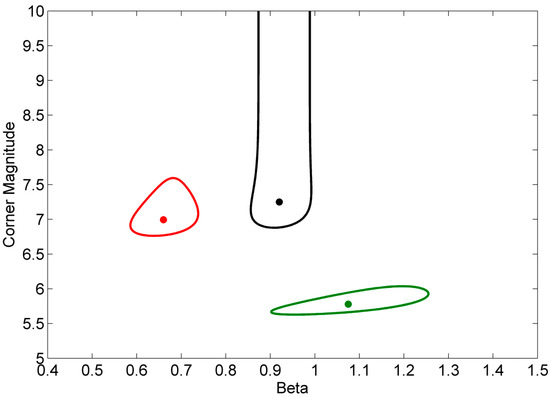
Figure 7.
95% Confidence region estimation (curves) and maximum likelihood estimations MLEs (dots) for the whole catalog (black), and the sub-catalogs with strike-slip events (red), and with normal events (green).
Looking at the shape of the confidence regions, it is evident that the two parameters result fairly uncorrelated. Both for normal and strike-slip events we obtain closed confidence regions, i.e., the confidence regions define a finite area for the uncertainty, showing a well-constrained estimation for all parameters; conversely, for the whole catalog, the confidence region is open toward large corner magnitudes, indicating an unconstrained estimation of the corner magnitude [7,8]. These results are compatible with an infinite corner magnitude corresponding to an unbounded Gutenberg-Richter. We also obtain a clear distinction of the values for the two sub-catalogs, which results averaged when the whole catalog is used. In Table 3 we show all the MLE for the corner magnitude and parameters.
Table 3.
Maximum likely estimation MLE of the corner magnitude and the slope , for the whole catalog and for the two sub-catalogs.
5. Discussion
By adopting the newly developed procedure, we can consider a much larger dataset for estimating the parameters of the tapered Gutenberg-Richter distribution, as catalog should not be declustered and different magnitude of completeness can be adopted in an older time, extending the temporal coverture of the catalog. This allows a deeper analysis of the Gutenberg-Richter distribution, also considering possible variations in sub-catalogs.
We applied this principle to the seismicity of the Atlantic ridge, obtaining a much-improved description of its seismicity. In particular, the different shapes of the confidence regions obtained considering the whole catalog and the sub-catalogs clearly demonstrate that a mixture of different types of events (i.e., with different focal mechanisms) with different statistical properties for the Gutenberg-Richter distribution can lead to an untrustworthy estimation of its parameters, artificially enlarging their confidence bounds, in particular for the corner magnitude.
We find instead that the corner magnitude for both normal and strike-slip events is well constrained, and incompatible with an unbounded Guttenberg-Richter distribution. This is in agreement with the observation that the size of such a structure is rather limited in the case of oceanic ridges [15]. The estimation of the corner magnitude for the normal event is particularly low ( = 5.78), but it is in line with the estimation obtained by Bird et al. [15] for oceanic spreading ridge earthquakes ( = 5.83). Conversely, the undifferentiated catalog provides an averaged corner magnitude (biased with respect to both sub-catalogs), with an open confidence region that is compatible with unbounded distribution. Notably, the sub-catalogs almost completely cover the entire catalog, and the thrust and unclassified events not only represent a small subset of events, but also cannot influence the estimation of the corner magnitude, as the maximum observed magnitude for these events is considerably smaller than the one of the whole catalog (6.31 vs. 7.10).
The slope parameter for strike-slip event is similar to the one of Schorlemmer et al. [29] for the global catalog; on the contrary, the for the normal events is very high (), corresponding to a b-value equal to 1.62; however, this estimation is quite uncertain (see Figure 7, green curve), with the 95% confidence region for ranging from 0.90 to 1.25. This large confidence region is compatible with the estimated by Bird and Kagan [16] for the normal event in the oceanic spreading ridge ().
The results are pretty independent of the selected completeness. In the Supplementary Material, we perform the same estimation shown in Figure 7, but using a more conservative magnitude of completeness, obtaining very similar results, and thus demonstrating that these results are robust and do not depend on the chosen completeness thresholds.
As discussed above, the newly developed estimation method allows increasing the input dataset by not requiring declustering and by allowing a variation through time of the completeness level. While the largest reduction is due to no declustering, we not that also the possibility of considering different completeness levels has a considerable impact. In Figure 8 we show the specific impact of the use of different completeness thresholds through time, allowed by the newly developed estimation method. The results are compared with the classical estimation method, in which one level of completeness for the whole catalog is used (Mw 5.5 from 1980 to 2019). The lower number of events available using only one level of completeness leads to larger confidence regions. In particular, for normal events, the confidence region computed with the classical method (light green curve in Figure 8) is much bigger than the one computed with the new method (green curve in Figure 8). As expected, a larger amount of available information leads to smaller uncertainties in the estimated parameters, especially in this case. Notably, central values (MLEs) also change, correcting potential biases. For example, the MLE for the entire catalog results outside the confidence bounds defined using more data.
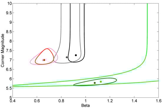
Figure 8.
95% Confidence region estimation (curves) and maximum likelihood estimations MLEs (dots) for the classical estimation approach (light colors: gray, pink, and light green) and the new estimation approach (dark colors: black, red, and green). As in Figure 7, we report both results using for the whole catalog (gray and black), and the sub-catalogs with strike-slip events (pink and red), and with normal events (light green and green).
The different shapes of the confidence region considering the whole catalog and the sub-catalogs show the importance of separating the contribution of different classes of earthquakes to correctly interpret their behavior. Indeed, the averaged behavior estimated from the complete catalog is substantially incompatible with the actual behavior of each single seismicity class. Indeed, by applying the global statistics (obtained by the full catalog) to each individual class, we would implement the wrong statistics to different classes, impacting the hazard in a different way. In our case study for the Atlantic ridge, we would artificially increase the probability of high magnitude normal events. On the contrary, compared with strike-slip events, we demonstrated that normal earthquakes have a significantly smaller corner magnitude coupled with a significantly larger b-value, resulting in a smaller probability of high magnitude normal events.
This not only may complicate the interpretation of the parameter estimation, but also may have a significant impact on hazard quantifications. For example, most of the recent ground motion prediction equations to estimate the attenuation of seismic waves from the source to target are dependent on faulting mechanisms, applying different attenuation laws to the different mechanisms (e.g., [30]). This is probably even more impacting is tsunami hazard, where different mechanisms have a different capability of deforming the sea bottom, resulting in different tsunamigenic capabilities (e.g., [31]). For example, normal events are typically more tsunamigenic than strike-slip events. For not introducing artificial bias in hazard quantification, it will be therefore fundamental to individuate potential mechanism-dependent variation of earthquake statistics and apply hazard models allowing for the aggregation of multiple classes of seismicity (e.g., [32]).
6. Conclusions
The main findings of this work can be summarized by the following two points:
- (1)
- We introduce a new method to estimate the parameters of the tapered Gutenberg-Richter distribution and their uncertainties in the case of catalogs with a variable through-time magnitude of completeness;
- (2)
- We apply this method to the Atlantic ridge seismicity, finding a clear distinct behavior both for the parameters and corner magnitude, depending on the faulting mechanism: larger and smaller corner magnitude for normal events, smaller and larger corner magnitude for strike-slip events.
Supplementary Materials
The following are available online at https://www.mdpi.com/article/10.3390/app112412166/s1. Figure S1: 95% confidence region estimation (curves) and MLE (dots) for the whole catalog (black), strike-slip events (red), and normal events (green) (completeness thresholds +0.1); Figure S2: 95% confidence region estimation (curves) and MLE (dots) for the whole catalog (black), strike-slip events (red), and normal events (green) (completeness thresholds +0.2).
Author Contributions
M.T. and J.Z. conceived the method; M.T. and J.S. defined the application; M.T. performed the data analysis and created the figures; M.T. and J.S. wrote the paper. All authors have read and agreed to the published version of the manuscript.
Funding
This work benefited of the agreement between Istituto Nazionale di Geofisica e Vulcanologia and the Italian Presidenza del Consiglio dei Ministri, Dipartimento della Protezione Civile (DPC), and of the project “Assessment of Cascading Events triggered by the Interaction of Natural Hazards and Technological Scenarios involving the release of Hazardous Substances”, funded by the Italian Ministry MIUR PRIN (Progetti di Ricerca di Rilevante Interesse Nazionale) 2017—Grant 2017CEYPS8.
Institutional Review Board Statement
Not applicable.
Informed Consent Statement
Not applicable.
Data Availability Statement
Data and code used in this paper are available at: https://github.com/MatteoTaroniINGV/TaperedGR_Estimation_Catalogs_with_variable_completeness (accessed on 8 July 2021).
Acknowledgments
The authors thank the two anonymous reviewers for their comments which greatly improved the paper.
Conflicts of Interest
Authors declare no conflict of interest.
Abbreviations
| Abbreviation | Meaning |
| Mmax | Maximum magnitude |
| MLE | Maximum likelihood estimation |
| Mmin | Magnitude of completeness |
| CMT | Centroid moment tensor catalog |
| CM | Corner magnitude |
References
- Gutenberg, B.; Richter, C.F. Frequency of earthquakes in California. Bull. Seismol. Soc. Am. 1944, 34, 185–188. [Google Scholar] [CrossRef]
- Aki, K. Maximum likelihood estimate of b in the formula logN = a − bM and its confidence limits. Bull. Earthq. Res. Inst. 1965, 43, 237–239. [Google Scholar]
- Kagan, Y.Y. Seismic moment distribution revisited: I. Statistical results. Geophys. J. Int. 2002, 148, 520–541. [Google Scholar] [CrossRef]
- Zöller, G.; Holschneider, M. The earthquake history in a fault zone tells us almost nothing about mmax. Seismol. Res. Lett. 2016, 87, 132–137. [Google Scholar] [CrossRef]
- Holschneider, M.; Zöller, G.; Hainzl, S. Estimation of the maximum possible magnitude in the framework of a doubly truncated Gutenberg–Richter model. Bull. Seismol. Soc. Am. 2011, 101, 1649–1659. [Google Scholar] [CrossRef]
- Zöller, G.; Holschneider, M.; Hainzl, S. The maximum earthquake magnitude in a time horizon: Theory and case studies. Bull. Seismol. Soc. Am. 2013, 103, 860–875. [Google Scholar] [CrossRef]
- Geist, E.L.; Parsons, T. Undersampling power-law size distributions: Effect on the assessment of extreme natural hazards. Nat. Hazards 2014, 72, 565–595. [Google Scholar] [CrossRef]
- Kagan, Y.Y.; Schoenberg, F. Estimation of the upper cutoff parameter for the tapered Pareto distribution. J. Appl. Probab. 2001, 38, 168–185. [Google Scholar] [CrossRef]
- Schoenberg, F.P.; Patel, R.D. Comparison of Pareto and tapered Pareto distributions for environmental phenomena. Eur. Phys. J. Spec. Top. 2012, 205, 159–166. [Google Scholar] [CrossRef]
- Kijko, A.; Sellevoll, M.A. Estimation of earthquake hazard parameters from incomplete data files. Part I. Utilization of extreme and complete catalogs with different threshold magnitudes. Bull. Seismol. Soc. Am. 1989, 79, 645–654. [Google Scholar] [CrossRef]
- Weichert, D.H. Estimation of the earthquake recurrence parameters for unequal observation periods for different magnitudes. Bull. Seismol. Soc. Am. 1980, 70, 1337–1346. [Google Scholar] [CrossRef]
- Taroni, M.; Selva, J. GR_EST: An OCTAVE/MATLAB Toolbox to Estimate Gutenberg–Richter Law Parameters and Their Uncertainties. Seismol. Res. Lett. 2021, 92, 508–516. [Google Scholar] [CrossRef]
- Kagan, Y.Y. Earthquake number forecasts testing. Geophys. J. Int. 2017, 211, 335–345. [Google Scholar] [CrossRef][Green Version]
- Taroni, M.; Akinci, A. Good practices in PSHA: Declustering, b-value estimation, foreshocks and aftershocks inclusion; a case study in Italy. Geophys. J. Int. 2021, 224, 1174–1187. [Google Scholar] [CrossRef]
- Bird, P.; Kagan, Y.Y.; Jackson D., D. Plate tectonics and earthquake potential of spreading ridges and oceanic transform faults. In Plate Boundary Zones; Stein, S., Freymueller, J.T., Eds.; AGU: Washington, DC, USA, 2002; Volume 30, pp. 203–218. [Google Scholar]
- Bird, P.; Kagan, Y.Y. Plate-tectonic analysis of shallow seismicity: Apparent boundary width, beta, corner magnitude, coupled lithosphere thickness, and coupling in seven tectonic settings. Bull. Seismol. Soc. Am. 2004, 94, 2380–2399. [Google Scholar] [CrossRef]
- Kanamori, H. The energy release in great earthquakes. J. Geophys. Res. 1977, 82, 2981–2987. [Google Scholar] [CrossRef]
- Vere-Jones, D.; Robinson, R.; Yang, W. Remarks on the accelerated moment release model: Problems of model formulation, simulation and estimation. Geophys. J. Int. 2001, 144, 517–531. [Google Scholar] [CrossRef]
- Kagan, Y.Y.; Bird, P.; Jackson, D.D. Earthquake patterns in diverse tectonic zones of the globe. Pure Appl. Geophys. 2010, 167, 721–741. [Google Scholar] [CrossRef]
- Wilks, S.S. Mathematical Statistics; Wiley: New York, NY, USA, 1962. [Google Scholar]
- Venzon, D.J.; Moolgavkar, S.H. A method for computing profile-likelihood-based confidence intervals. J. R. Stat. Soc. Ser. C Appl. Stat. 1988, 37, 87–94. [Google Scholar] [CrossRef]
- Dziewonski, A.M.; Chou, T.-A.; Woodhouse, J.H. Determination of earthquake source parameters from waveform data for studies of global and regional seismicity. J. Geophys. Res. 1981, 86, 2825–2852. [Google Scholar] [CrossRef]
- Ekström, G.; Nettles, M.; Dziewonski, A.M. The global CMT project 2004–2010: Centroid-moment tensors for 13,017 earthquakes. Phys. Earth Planet. Inter. 2012, 200–201, 1–9. [Google Scholar] [CrossRef]
- Mizrahi, L.; Nandan, S.; Wiemer, S. The effect of declustering on the size distribution of mainshocks. Seismol. Res. Lett. 2021, 92, 2333–2342. [Google Scholar] [CrossRef]
- Marzocchi, W.; Spassiani, I.; Stallone, A.; Taroni, M. How to be fooled searching for significant variations of the b-value. Geophys. J. Int. 2020, 220, 1845–1856. [Google Scholar] [CrossRef]
- Lilliefors, H.W. On the Kolmogorov-Smirnov test for the exponential distribution with mean unknown. J. Am. Stat. Assoc. 1969, 64, 387–389. [Google Scholar] [CrossRef]
- Taroni, M. Back to the future: Old methods for new estimation and test of the Gutenberg-Richter b-value for catalogs with variable completeness. Geophys. J. Int. 2021, 224, 337–339. [Google Scholar] [CrossRef]
- Zhuang, J.; Ogata, Y.; Wang, T. Data completeness of the Kumamoto earthquake sequence in the JMA catalog and its influence on the estimation of the ETAS parameters. Earth Planets Space 2017, 69, 1–12. [Google Scholar] [CrossRef]
- Schorlemmer, D.; Wiemer, S.; Wyss, M. Variations in earthquake-size distribution across different stress regimes. Nature 2005, 437, 539–542. [Google Scholar] [CrossRef] [PubMed]
- Douglas, J.; Edwards, B. Recent and future developments in earthquake ground motion estimation. Earth-Sci. Rev. 2016, 160, 203–219. [Google Scholar] [CrossRef]
- Grezio, A.; Babeyko, A.; Baptista, M.A.; Behrens, J.; Costa, A.; Davies, G.; Geist, E.; Glimsdal, S.; Gonzales, F.I.; Griffin, J.; et al. Probabilistic Tsunami Hazard Analysis: Multiple Sources and Global Applications. Rev. Geophys. 2017, 55. [Google Scholar] [CrossRef]
- Selva, J.; Tonini, R.; Molinari, I.; Tiberti, M.M.; Romano, F.; Grezio, A.; Melini, D.; Piatanesi, A.; Basili, R.; Lorito, S. Quantification of source uncertainties in Seismic Probabilistic Tsunami Hazard Analysis (SPTHA). Geophys. J. Int. 2016, 205, 1780–1803. [Google Scholar] [CrossRef]


Publisher’s Note: MDPI stays neutral with regard to jurisdictional claims in published maps and institutional affiliations. |
© 2021 by the authors. Licensee MDPI, Basel, Switzerland. This article is an open access article distributed under the terms and conditions of the Creative Commons Attribution (CC BY) license (https://creativecommons.org/licenses/by/4.0/).