1. Introduction
Tunnel boring machines (TBMs) are currently the most utilized equipment for deep and long tunnels in both civil and mining industries. One important consideration prior to the actual excavation is evaluating ground conditions along the proposed tunnel alignment. This initial evaluation provides critical information for selecting the excavation type and developing preliminary ground support systems. Ground conditions are obtained by the characterization and subsequent classification of the rock mass based on a pre-defined system known as a rock mass classification system. Since the introduction of rock mass classification by Terzaghi, it has become a useful tool for rock engineering and is widely considered the most practical method for evaluating the quality of the rock mass in underground engineering practices. The common and widely used classification systems are the Q-system [
1], Rock Mass Rating (RMR) [
2], Rock Mass Index (RMi) [
3], and Geological Strength Index (GSI) [
4]. Aside from these classification systems, the Japanese Highway Classification System (JH system) and the Hydropower Classification System (HC system) are also popular in Asia.
One of the serious concerns in the use of rock mass classifications schemes is that they are subjective. Field engineers with different experience levels classifying the same rock mass using for example, RMR, can produce significantly different rock mass behavior [
5]. This is because most of these classification systems use both quantitative and qualitative methodologies. To reduce, if not to eliminate, the subjectivity or experience factor in rock mass classification, a data-driven system is necessary. Some of the early attempts on data-driven approaches focused on the use of non-destructive forward geological prospecting techniques including tunnel seismic prediction (TSP), and ground penetration radar (GPR) to assess the rock mass quality ahead of TBMs [
6,
7]. Although these geophysical techniques provide reliable and accurate results, they are expensive and cause undue project delays. Zhang et al. [
8] indicated that these forward geophysical prospecting techniques are not directly related to the rock tunneling/excavation process since they can only be implemented when the TBM is not in operation. Besides the subjective nature of rock mass classification systems, limited space between the TBM cutterhead and the tunnel face makes geologic mapping for classifying in-situ ground conditions difficult, if not impossible [
9].
Another data-driven approach for classification of rock mass conditions in tunnels excavated by TBMs is the application of artificial intelligence (AI) and machine learning (ML) techniques to TBM operating parameters. Several researchers [
10,
11,
12,
13,
14,
15,
16,
17] have applied ML algorithms, capable of handling complex non-linear problems, to establish the relationship between TBM operational data and rock mass conditions. Liu et al. [
18] used cutterhead thrust, cutterhead torque, revolution per minute (RPM), and penetration rate to develop a simulated annealing-back propagation neural network (SA-BPNN) model to predict rock mass properties (UCS, brittleness index (Bi), and the distance between plane of weakness (DPW). Current research in rock excavation and tunneling is focused on developing reliable AI and ML models based exclusively on TBM operational data.
The overall objective of these efforts is to develop some kind of on-board rock mass classification system on TBMs that will allow automated rock mass classification and possibly ground support system selection. Liu et al. [
19] used TBM operational data to train a support vector classifier coupled with genetic algorithm to classify rock masses based on the improved basic quality (BQ) classification system. Jung et al. [
20] applied ANN to shield TBM operational data (penetration rate, cutterhead torque and thrust force) to predict ground conditions ahead of the TBM. Zhang et al. [
8] used RF, K-NN, and support vector classification (SVC) to predict ground conditions in tunnels using four TBM parameters namely; cutterhead torque, cutterhead thrust, cutterhead speed, and advance rate, and concluded that SVC outperformed the other techniques with an accuracy of 98%. They also indicated that out of the four TBM parameters analyzed, the cutterhead torque and thrust were found to better reflect the changes in rock types. Based on the Hydropower classification (HC) system, [
9] used TBM operational data to train five predictive models: AdaBoost-CART, CART, SVC, ANN, and KNN, and concluded that AdaBoost-CART was the best model for predicting rock mass conditions. Zhang et al. [
21] used ANN, SVM, KNN, and CART to develop geologic type recognition classifiers based on advance rate, cylinder thrust, cutterhead torque, and cutterhead rotational speed. Erharter and Marcher [
22] proposed the multivariate sequence segmentation, abstraction, and classification (MSAC), a data-driven rock mass classification model, using the advance force, cutterhead torque, penetration rate, cutterhead rotations, advance speed, specific penetration, specific energy, and torque ratio.
This study explores the suitability of two supervised machine learning algorithms, random forest (RF), and extremely randomized trees (ERT) in predicting the ground conditions on the tunnel face ahead of a TBM based on the Japanese Highway Classification System. RF and ERT harness the predictive capabilities of multiple decision trees. Different sets of predictors are used at each node; hence, the variance of the resulting model is significantly reduced compared to the individual regression trees. RF was selected for this analysis because it has been applied successfully in a wide variety of projects and has seen tremendous acceptance in many disciplines due to its tendency to decrease the models’ variance [
23]. ERT, on the other hand, is relatively unknown especially in the area of rock excavation but it was selected due to its high performance with less noisy data. In this study, TBM operating parameters namely; rate of penetration, cutterhead torque, cutterhead thrust force, cutterhead revolution per minute, hydraulic cylinder stroke speed, boring pressure, pitching, and motor amps were analyzed using the two ML algorithms to develop models for classifying the rock mass conditions in TBM tunnels. This research contributes to the ongoing research efforts towards developing reliable models that could be incorporated into TBMs to allow for on-the-fly characterization and classification of ground conditions in tunnel excavation as well as eventual automation of ground support systems selection.
1.1. The Japanese Highway Classification System (JH System)
The Japanese Highway Classification System was first developed in Japan in the 1960s for large dam foundation and later extended to tunnel rock mass characterization [
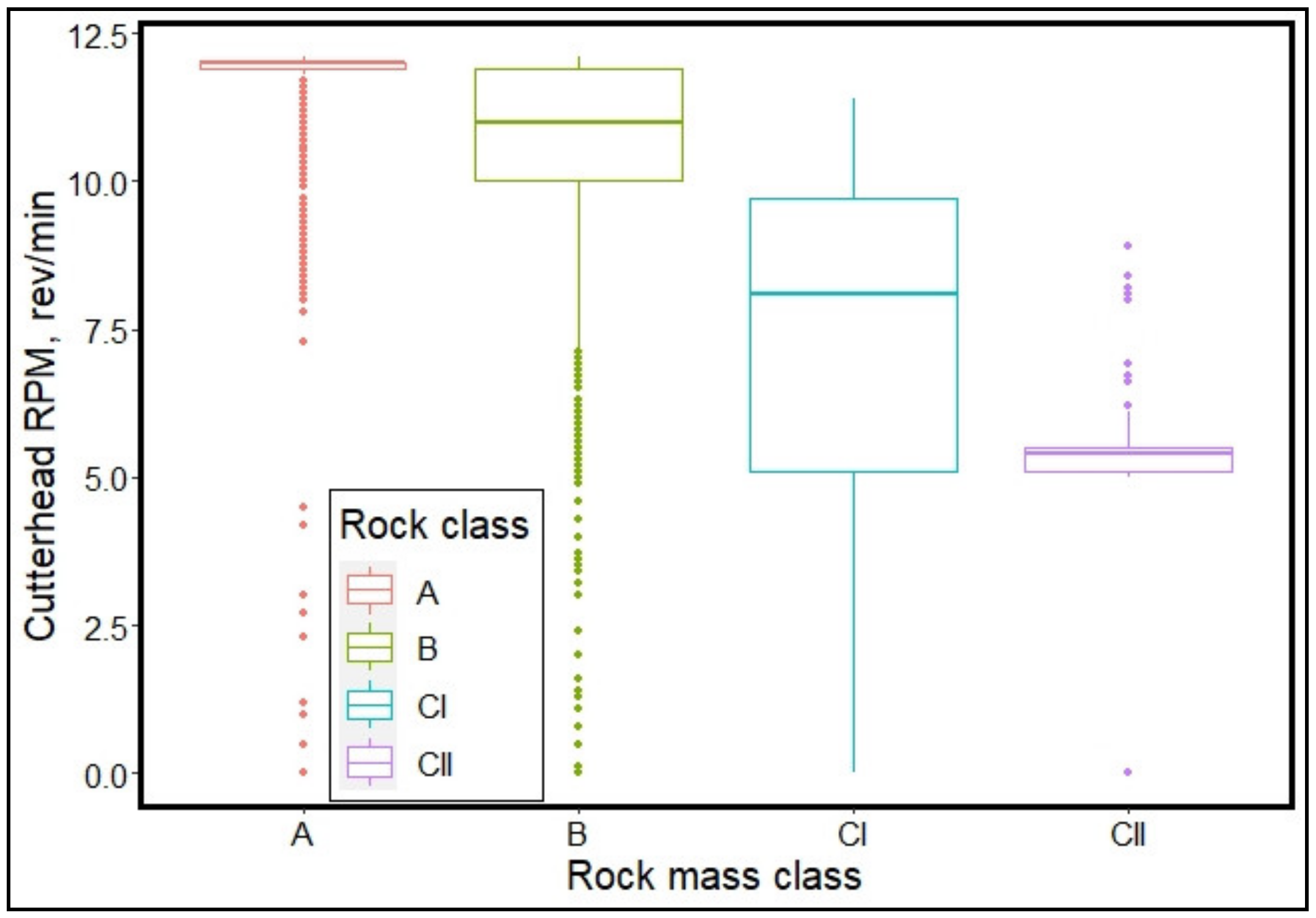
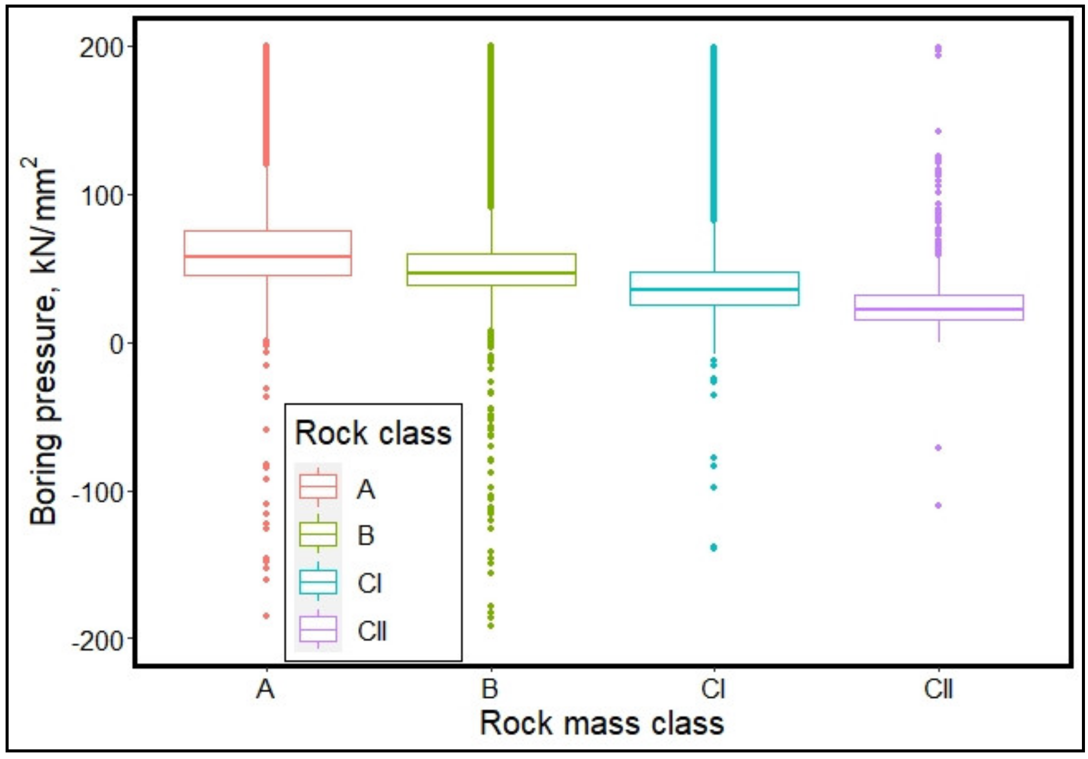
24]. This classification system commonly referred to as JH System, like many rock mass classification systems, has undergone several revisions since its introduction. The JH System relies primarily on seven rock mass parameters namely: intact rock strength (compressive strength), weathering, spacing of discontinuities, condition of discontinuities, effect of discontinuities orientation, groundwater condition, and degradation by water. Each of these parameters is further subdivided into subgrades and assigned a grade point corresponding to the level of the rock mass feature being characterized. For example, the intact rock property (UCS), is divided into six subgroups: less than 3 MPa, 3–10 MPa, 10–25 MPa, 25–50 MPa, 50–100 MPa, and greater than 100 MPa. Each of these subgroups is assigned a grade point reflecting the strength of the intact rock material.
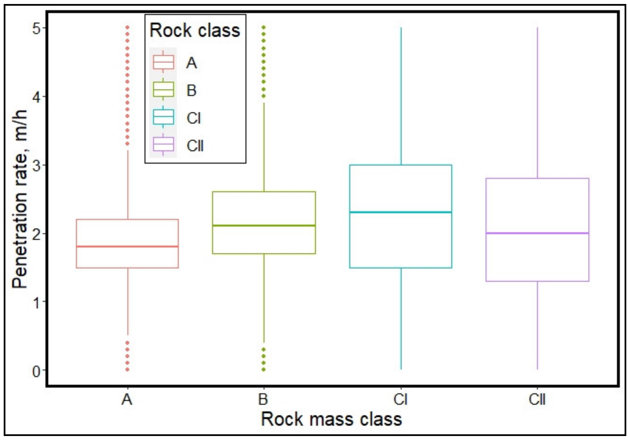
Once each rock mass parameter is graded/rated, the grade point for the intact rock property, weathering, joints spacing, condition of joints are added up and the grade points for groundwater conditions, deterioration due to water, and effect of discontinuities orientation are subtracted from the sum to obtain total grade points of the rock mass at that location. The total grade point ranges from 0 to 100 representing very poor rock to very good fresh rock respectively. The total grade point is then used to categorize the rock mass into classes. The system has six rock mass classes; A, B, CI, CII, D, and E. In terms of rock mass competence, it decreases from class A through class E, with class E been the least competent rock mass. In tunnel excavation, these rock mass groups are used to determine the ground support system required to stabilize the tunnel walls.
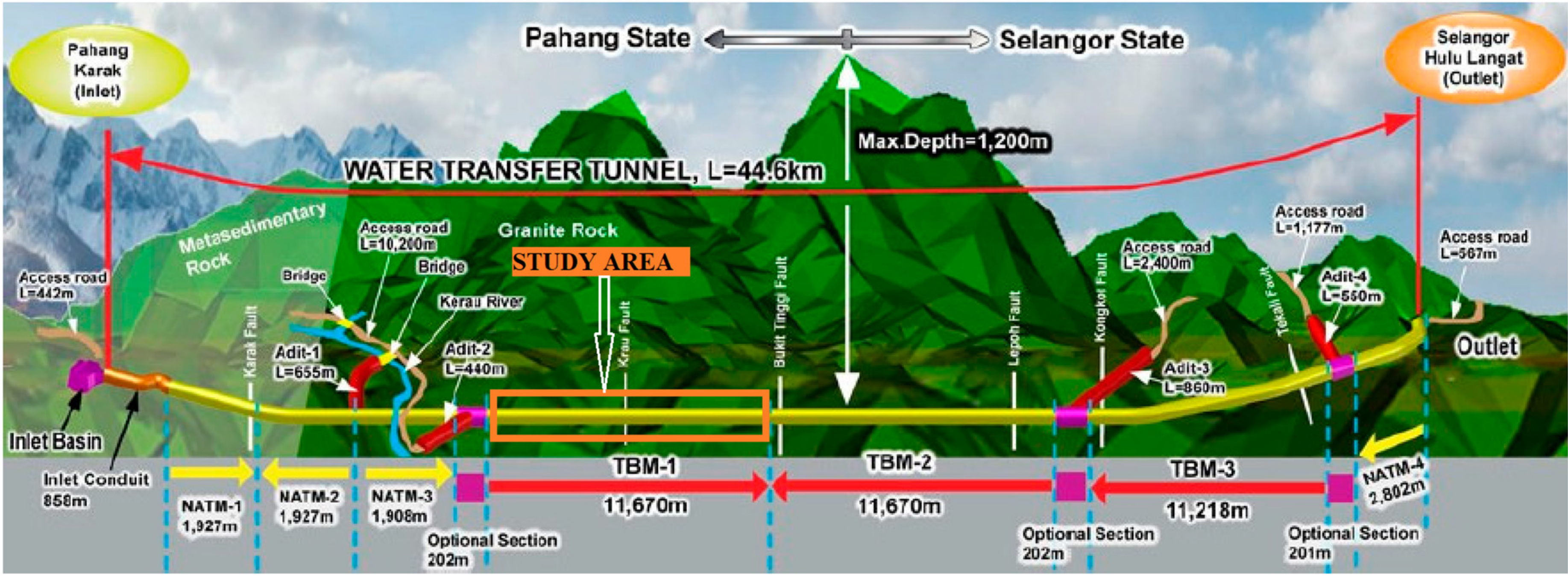
Table 1 shows typical JH System data collection sheet used in the Pahang-Selangor Raw Water Tunnel (PSRWT) while
Table 2 shows typical ground support systems for the different rock mass classes.
4. Development of Machine Learning (ML) Models
Two machine learning techniques, random forest, and extremely randomized trees, were applied to develop models for classifying the rock mass dataset into categories based on JH rock classification system. This section discusses the data preprocessing, machine learning models that were applied, and their learning process.
4.1. Data Preprocessing
The TBM operation parameters were recorded at a much higher resolution, about a fraction of a meter, as compared to the rock mass data, which were collected every 4 to10 m. The rock mass data was taken at a coarse resolution because the rock properties in this section of the tunnel were not changing much within a short interval. Where a change in rock mass characteristics was observed, a finer rock mass data collection resolution was used in order to capture all the variations in the rock mass. Another possible reason for coarser resolution in the rock mass data is that taking the rock mass data involves shutting down the operations to allow for geologist to be able to access the tunnel walls. On the other hand, the machine operating parameters are easier to collect and does not require any downtime. For this study, the resolution of the machine data and the rock mass data had to be matched to enable usage of the machine data to predict the rock mass conditions. The chainage interval in the two datasets was used as a key to match the two datasets. That is, the rock mass record for a particular chainage interval is adjoined to all the TBM records in that chainage interval. This was done for all the data points in the rock mass dataset, creating the aggregate dataset used for this study.
The variables in the dataset consist of a wide range of scales, tens to thousand. Consequently, the data was normalized so that the input variables are in the same scale. According to Jayalakshmi and Santhakumaran [
26], normalization helps minimize bias caused by different scales of the input variables. Computational speed is also improved by data normalization since the features are put on the same scale. As a result, that dataset in this study was normalized using the min-max normalization which preserves the relationship between the input and output variables. The input variables were scaled to a range between a minimum of zero and a maximum of one. The preProcess() function in R software was used to normalize the data in this study. The normalization is achieved using Equation (1) [
26].
where
is the rescaled feature x,
is the maximum value of feature x,
is the minimum value of feature x, and
is the ith value of feature x.
4.2. ML Models Description
4.2.1. Random Forest (RF)
According to Zhang and Ma [
23], random forest (RF) has been applied successfully in a wide variety of projects and has seen tremendous acceptance in many disciplines, thus, its inclusion in this study. RF also has the capability of ranking the importance of all the input variables contributing to the prediction of the target variable.
The predictive abilities of multiple decision trees are harnessed by Random Forest, an ensemble method. To practice each decision tree, bootstrapped samples are used and the predictive capabilities of all the trained trees are aggregated to form the final model. A number of predictors,
mtry, was randomly chosen in constructing the trees to be considered at each node during the recursive binary splitting instead of using all the predictors [
27]. This gives the technique its name, random forest. At each node, a different set of predictors are used for node splitting; therefore, the variance of the resulting model is significantly reduced compared to the individual regression tree. In training the decision trees, each split is done to obtain two regions
R1 and
R2 as in Equation (2).
where
j is the index in the predictor space with an upper limit of
mtry and
s is the cut point for the split.
The objective is to obtain
j and
s values that minimize the function (Equation (3)).
with
is the mean response for the training observations in
R1(
j, s); and
is the mean response for the training observations in
R2(
j, s).
This process is repeated until there is no decrease in residual sum of squares by further splitting, at which point the terminal node is reached. The number of predictors to be considered in the splitting at the nodes,
mtry, is a hyperparameter that has been calibrated using 5-fold cross-validation (CV) to achieve an optimum value for the best prediction output in training the random forest model [
27]. The optimal
mtry was then used to fit the final model.
4.2.2. Extremely Randomized Tree (ERT)
ERT is also an ensemble method similar to RF. The difference between RF and ERT is in the mode of tree nodes splitting. While the splitting is deterministic in RF, it is randomized in ERT. The randomized splitting in ERT has the tendency to further reduce the prediction variance when the dataset has a low level of noise. This implies that when the dataset is less noisy, ERT tends to perform significantly better than RF. However, when the data is noisy ERT does not necessarily have an improved performance over RF. Due to the randomized nature of node splitting, ERT is more computationally expensive than RF. Therefore, if the performance of ERT is not significantly better than that of RF, it is recommendable to adopt RF. A detailed description of ERT can be found in [
28]. ERT is considered in this study because of its semblance to the RF model which has proven to be effective in predicting mechanical excavator’s performance [
29] and its tendency to have improved performance over RF.
4.3. Machine Learning Process
Since the response variable—rock mass class—has four levels, multi-class classification was conducted using Random Forest and Extremely Randomized Trees. The models were trained on 70% of the dataset and the remaining 30% was used to evaluate their classification performance. These fractions were chosen because the dataset is large and oversampling of the minority classes in the training set further increased the size of the training set, hence, 70% of the data was used for the model training instead of the usual 80% that is generally used.
During the model training, 5-fold CV was used to tune the hyperparameters of the models. In RF, the hyperparameter,
mtry, is the number of predictors that are considered in deciding the best split at each decision node [
27]. The
mtry for this dataset was 5. The hyperparameters for the ERT are
mtry and
numRandomCuts. numRandomCuts is the number of randomly selected splits for each
mtry. The
mtry and
numRandomCuts in this study were both 6. After obtaining the optimal hyperparameters the cross-validation run, the final models were then fitted using these hyperparameters.
4.4. ML Model Performance Metrics
4.4.1. Accuracy and Balanced Accuracy
Accuracy is the measure of correct classifications. It is the ratio of the number of observations that are correctly classified to the total number of observations. This metric is only meaningful when evaluating balanced datasets. It loses its relevance when evaluating an unbalanced dataset [
30]. In studies involving unbalance datasets, balanced accuracy is a more meaningful performance metric. It is calculated as the average of the proportion corrects of each class individually, that is, the arithmetic mean of the precision and recall (Equation (4)).
where
b is the balance accuracy,
p is the precision, and
re is the recall
4.4.2. F1 Score
Precision measures the proportion of positive classifications that are correct in binary classification. It is the ratio of the number of correct positive classifications to the total number of positive observations [
30]. Recall is a measure of the proportion of actual positives that are identified correctly. This is also known as the sensitivity of the model [
30]. There is usually a trade-off between precision and recall depending on the purpose of the classification and the risk associated with the false-positive classification. The
F1 score is the harmonic mean of precision and recall (Equation (5)).
4.4.3. Cohen’s Kappa Coefficient (k)
Kappa is a statistical measure of the agreement between different raters [
31]. In this case, it is the measure of the agreement between the predicted and observed rock mass classes. Unlike accuracy, kappa takes into account classifications made by chance. It is given by Equation (6). The following descriptions are given to various ranges of kappa: 0 = agreement equivalent to chance; 0.1–0.20 = slight agreement; 0.21–0.40 = fair agreement; 0.41–0.60 = moderate agreement; 0.61–0.80 = substantial agreement; 0.81–0.99 = near perfect agreement; 1 = perfect agreement [
31]. In formula,
where
is the relative observed agreement among raters; and
is the hypothetical probability of chance agreement.
6. Conclusions
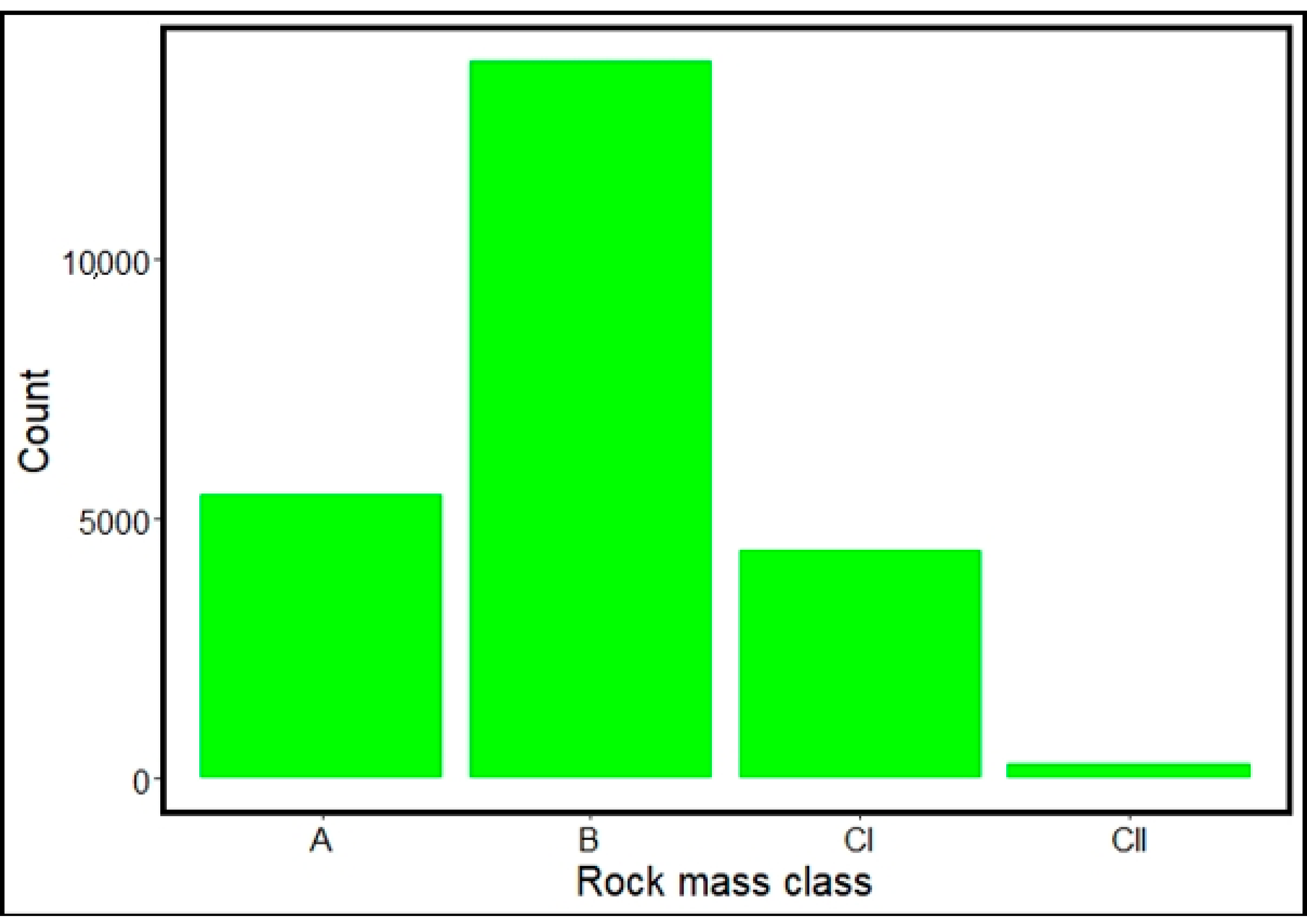
In this study, two machine learning (ML) classification algorithms; random forest and extremely randomized trees, were employed to characterize and classify ground conditions along the Pahang-Selangor Raw Water Transfer (PSRWT) tunnel alignment in Malaysia based on TBM operating parameters and rock mass data obtained based on JH rock mass classification system. The TBM operating parameters included in this approach are rate of penetration, cutterhead torque, cutterhead thrust, cutterhead revolution per minute, hydraulic cylinder stroke speed, boring pressure, and motor amps. Due to imbalance in the rock mass data, an oversampling technique was used to obtain a balanced training dataset for unbiased learning of the machine learning (ML) models. Multi-class classification was done, categorizing the rock mass condition into A, B, CI, and CII classes per the JH system. The JH classification system categorizes rock mass into six classes but the tunnel section from which the dataset was obtained consisted primarily of hard rocks. Consequently, only rock classes consistent with hard rock were encountered and analyzed in this paper. An extension of this study is needed with a dataset that includes all the soft rock mass classes to make the developed models compressive in all ground conditions that the TBM may encounter along the tunnel tract.
The main conclusions of this study can be summarized as follows:
The proposed approach was applied to a dataset from the Pahang-Selangor Raw Water tunnel (PSRWT) project in Malaysia. A comparison between the ML model classification results and the measured rock mass classes shows that the proposed approach is effective. The identification and classification accuracies were 95% and 94% for ERT and RF, respectively with kappa values of at least 0.90.
A bootstrap comparison of the performance of the two ML models, RF and ERT, indicated no model outperformed the other. Due to the randomized nature of node splitting, ERT is more computationally expensive than RF. Therefore, if the performance of ERT is not significantly better than that of RF, it is recommendable to adopt RF.
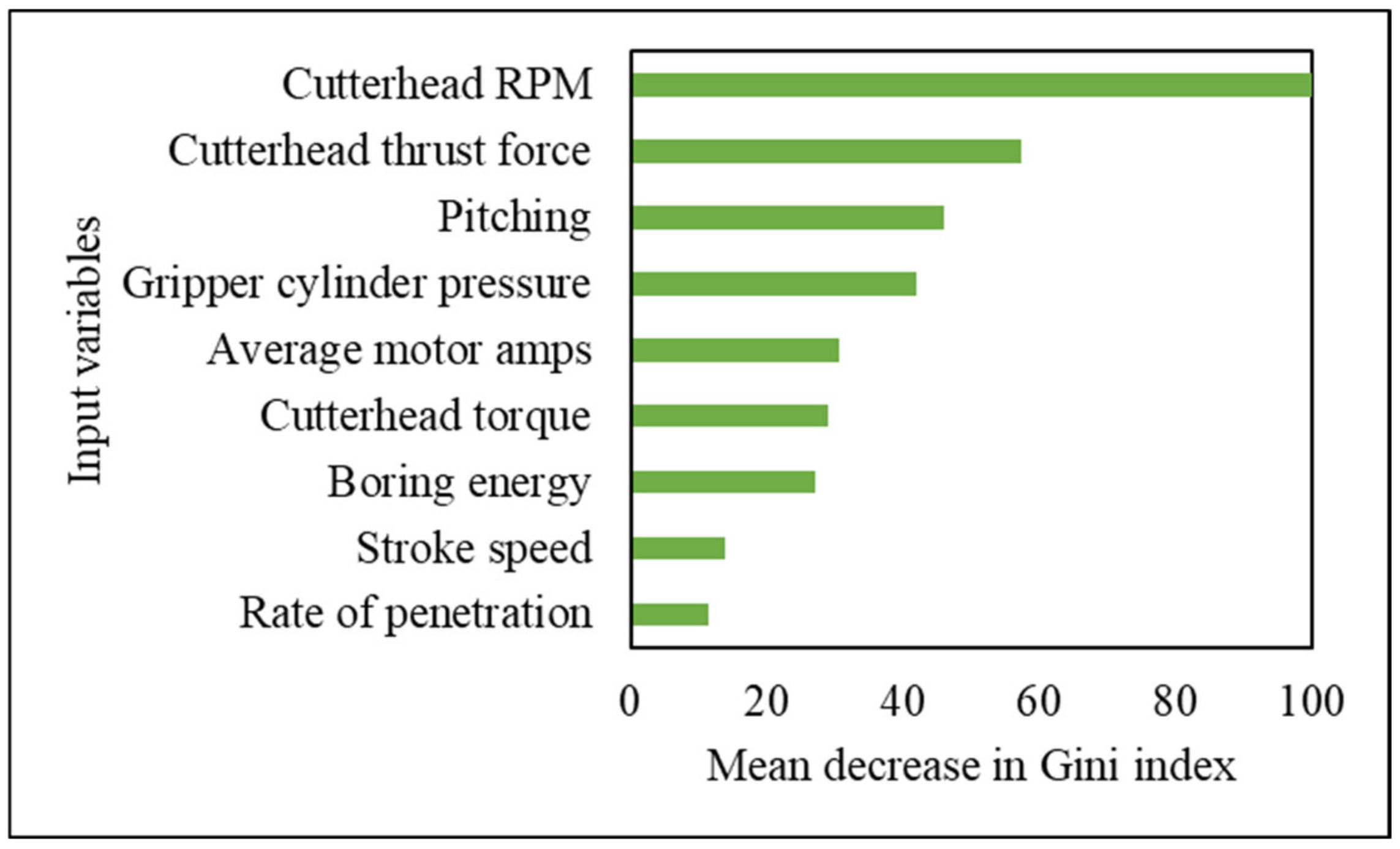
The most influential TBM operating parameter in classifying the rock mass is the cutterhead RPM followed by cutterhead thrust. The two least influential parameters are stroke speed and rate of penetration. Therefore, TBM thrust and RPM can be adjusted in real-time by determining the rock mass class being excavated using the ML models developed in this paper.
From a practical standpoint, the overall results obtained in this study show that the data-oriented approach is a useful tool for on-the-fly rock mass conditions identification, characterization and classification of ground conditions along tunnel alignment. It can be a tool for on-site decision making such as selecting support systems or refining preliminary support systems based on ground condition encountered.
Extension of this research should also focus on exploring other ML techniques including deep learning methods as well as developing a framework for operationalizing this approach in TBMs.

 ,
, 


