1. Introduction
In the second half of 19th century, the icy world of the world’s largest island started to attract the attention not only of various discoverers, who sought to unveil what was hidden in the so far unseen Greenland’s interior, but there was also an increasing number of scientific expeditions. To control such activities and to foster a more systematic exploration, in 1878 the Danish Interior Ministry established a Commission for Scientific Research in Greenland [
1]. After several unsuccessful attempts to overcome the very difficult weather and terrain conditions and to cross the island, in 1888 Norwegian explorer and scientist Fridtjof Nansen organized and led a small group of six people who finally succeeded in traversing the island on cross-country skis [
2]. Our paper is related to the following historical trek across Greenland, a 1912 expedition led by Swiss explorer Alfred de Quervain, which was the first to systematically measure the altitudes along the expedition’s 700 km traverse of the Greenland ice sheet [
3]. In 2002, a group of German researchers used de Quervain’s route to measure precise GNSS elevations and repeated such measurement campaigns several times with a few years’ separation (
Section 2).
Nowadays Greenland is the focus of researchers worldwide as well. Every year there are at least 100 scientific projects or investigations taking place in Greenland, about one third of which are Greenlandic or Danish, one third American, and the remainder from other countries with arctic research interests and traditions [
1]. Together, the ice sheets in Antarctica and Greenland contain about 70% of all freshwater on Earth and over 99% of freshwater ice; if melted completely, the Greenland ice sheet may cause the global sea level to rise by 7 m (e.g., [
4]). Another unique aspect of the Greenland ice sheet is the ice-drilling projects; starting in 1966, they have been helping in attempts to reconstruct the historical record of climatic and environmental conditions on Earth back to more than 100,000 years ago [
5]. Since the 1990s, there have been several space missions whose aim was to observe the state and physical conditions of Greenland. Both ground-based and satellite observations revealed that ice loss in Greenland has accelerated over the last two decades (
Section 6). As this is an important issue for the Earth as a planet, the current state of the Greenland ice sheet and its possible future climatic evolution are of great concern (for a review, see, e.g., [
6,
7,
8]).
In our paper, we want to compare locally measured GNSS positions with independent observations from satellites. Ground-based GNSS data provide reliable and precise information about the space coordinates of the measurement site at the uncertainty level of a few centimeters (
Section 2). On the other hand, satellite geodetic techniques cover broader regions of the surface at once, and thus each technique has its own advantages and disadvantages [
7,
9]. For the comparison with the altitude differences obtained from GNSS, we will use satellite radar altimetry data (
Section 4) and satellite gravimetry data from the GRACE mission (
Section 5). Laser and radar
satellite altimetry has better spatial resolution than satellite gravimetry, but it falls short of the high temporal resolution of GRACE. To convert the volume changes into mass changes, altimetry requires assumptions about the firn density. Because of radar signal penetration into the snow, altimetry has problems with the areas of large slopes, such as those around the ice sheet margin.
Satellite gravimetry provides direct measurements of mass and mass changes, but these are integrated vertically and one cannot distinguish between the individual sources, whether they are in the atmosphere, hydrosphere or cryosphere, or from the underlying solid Earth. Besides, the spatial resolution of satellite gravity is limited (250–500 km), so one cannot isolate a precise location of smaller anomaly sources (e.g., a glacier).
In polar regions, a particular effect is present, called
glacial isostatic adjustment or
postglacial rebound (e.g., [
9]). At the end of the last ice age (around 11,700 years ago), Northern Eurasia, Northern America, Patagonia and Antarctica underwent deglaciation, which until today causes the underlying crust to rebound. Thus, any error in the glacial isostatic adjustment model causes a similar height error in altimetry measurements. On the contrary, for gravimetry such an error is four to five times larger [
9]. This is because gravity observing instruments cannot distinguish between local gravity changes and a vertical displacement of the source material. Rock in the Earth mantle is four to five times as dense as ice, so its rise by 1 cm is equivalent to a rise of the surface ice sheet by 4–5 cm. We will pay attention to glacial isostatic adjustment; we will exclude it from the usual processing of satellite gravity data in order to be better comparable to the local GNSS observations (
Section 5); glacial isostatic adjustment will be included again in processing when estimating the total mass loss of the Greenland ice sheet (
Section 6).
In this paper, in
Section 2 the Greenland Korth Expeditions are introduced, during which the local GNSS measurements of the Greenland ice sheet were obtained. Then in
Section 3 the Greenland Korth Expeditions profile is displayed using satellite-derived maps of bed and surface elevations and the surface ice velocity.
Section 4 presents the comparison of the GNSS and radar altimetry observations, and in
Section 5 both satellite gravity and GNSS data are processed to be comparable. Finally,
Section 6 provides an updated estimate of the Greenland ice sheet mass change using recent satellite gravimetry measurements.
2. Greenland Korth Expeditions
In 2002 the project “Spurensuche” (in English: search for tracks), hereinafter called the Greenland Korth Expeditions (Greenland Korth Expeditions), was started. A four-person German expedition team under the direction of Wieland Adler crossed the Greenland ice sheet from Isotorq on the east coast to Port Victor (historically Quervains Havn) at Disko Bay on the west coast.
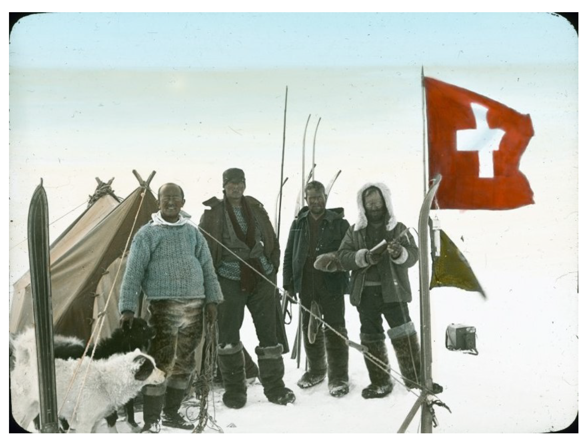
The historical model for this expedition was the 1912 Swiss Greenland expedition under the direction of Alfred de Quervain. After Fridtjof Nansen in 1888, this expedition was the second successful crossing of the Greenland ice sheet. They took a 700 km long traverse. Since the beginning, the Swiss expedition was meant to be a scientific exploration of the Greenland ice sheet. The group of four researchers carried out numerous geodetic and meteorological measurements. Alfred de Quervain (meteorologist and expedition leader), Hans Hössli (doctor), Karl Gaule (engineer) and Roderich Fick (architect, responsible for geodetic measurements) were members of the expedition that crossed the ice sheet using dog-sledges (
Figure 1). As a result of this expedition, the first elevation profile of the ice sheet was published [
10].
Ninety years later, this historic route was taken again and measured with modern GNSS technology. The scientific director was Wilfried Korth from the Technical College of Higher Education in Berlin (today: Beuth University of Applied Sciences Berlin).
Since the Greenland ice sheet is an important sensor for climate change, the results of repeated measurements over longer periods (e.g., height comparisons) can provide insight into this process. For this reason, in 2006 a group of six people crossed the ice sheet again [
11]. As in 2002, the direction of the expedition was given to Wieland Adler and the scientific direction to Wilfried Korth. Every four years, a group led by Wilfried Korth followed the footsteps of Alfred de Quervain [
12]. In 2010 a three-person group crossed the ice sheet and in 2012 a four-person anniversary expedition was planned, which had to be cancelled after about 100 km due to material damage [
13].
For the expeditions described above, a similar measuring program was implemented [
11]. The GNSS measurements were carried out with a Trimble Zephyr Geodetic antenna and the Trimble 5700, and later the Trimble R7, served as the receiver. Static GNSS measurements were carried out with observation times of several hours overnight at the campsites. In total, 35 measurements were made, together comprising the elevation profile presented here. Therefore, the following expeditions were tied to the places given in 2002. The expedition members had to reach them and use them as a campsite, even if the conditions were significantly worse or better. This procedure allowed made it possible to make an estimate about the shrinking or growing of the ice sheet at specific positions based on the differences in elevation. Certain tendencies can already be read from the repeated measurements, e.g., an increase in the melting process in the coastal areas.
In addition to the static measurements overnight, kinematic GNSS measurements were carried out at the camps. This was done in a radius of more than 100 m around the camp. The scatter plot of coordinates was then interpolated to a fitted plane. This simple adjustment with a standard deviation of a few centimeters is possible on snow and ice surfaces. Roughness does not disrupt the results [
14]. With the help of the grid and the interpolated plane, the points of the static measurement can be verified and the comparison with earlier measurements is possible with higher quality. This works also when the subsequent measurement does not take place at exactly the same point.
If the amount of ice movement is known in addition, by means of this approach a specific mass balance can be estimated [
14]. The inclination of the surface can be determined from the middle plane. The repeated measurement in 2006 showed no changes in inclination, which suggests a locally uniform melting or growth [
15].
Reference data from the International GNSS Service were used to correct the data [
11,
16]. An exception is the expedition in 2006, during which a reference station on the coast of Greenland was monitored by two students. The evaluation was carried out by different people with different software.
Trimble Total Control,
Trimble Business Center and
Bernese GNSS Software from the Astronomical Institute of the University of Bern were used.
Handheld GNSS devices were also used during each expedition since 2006. In addition to the geodetic measurements, meteorological data (temperature, atmospheric pressure, wind velocity, etc.) were recorded during the expeditions. Permanent magnets with a diameter of 45 mm, a thickness of 9 mm and a known magnetic moment were used as marks [
11]. After a return to the same location during the following expedition, these magnets reached a new position and depth due to the ice movements and accumulation. An area the size of a football/soccer field (100 m × 70 m) was scanned with a magnetometer at a grid spacing of 3 m in order to determine magnetic anomalies caused by the movement of the magnets. According to theoretical considerations, depth can be estimated from the maximum value of the magnetometer measurement at the surface (for more details, see [
11]). The signal gets weaker with increasing depth, and in the present case the limiting depth is about 5 m below the surface. In 2006 one particular magnet was dug up to check the real position and depth against the estimates of these two coordinates based on surface magnetometer measurements. Both the position (a position error of less than 30 cm) and the depth (magnetometer estimate: 4.1 m; actual depth: 4.12 m) were extremely precise. With this method, exact ice movements and the annual accumulation can be determined [
11]. A differentiation can be made between the accumulation area (increase; snow remains) and ablation area (loss of mass). In between, there is the equilibrium line or equilibrium zone.
Another successful crossing of the ice sheet took place in 2015 by a group of four under the direction of Wilfried Korth [
17]. For the first time, the route was examined with kinematic GNSS measurements in order to generate an almost continuous profile. With this method it is possible to compare the entire profile and not only the positions of the campsites. The Trimble R7 receiver and the NavXperience 3G+C antenna were used on the expedition. The antenna was screwed onto a frame that was braced on the pulka (
Figure 2a). Since this system was being tested for the first time, the static measurements continued overnight. A great advantage of the kinematic method was that the camps and measurement points set up in 2002 did not necessarily have to be reached and the length of the daily stages could be made dependent on the conditions. Nevertheless, a relatively large number of previous camps were reached enabling repeated measurements, so that the static measurements also remained significant. In addition, meteorological data were recorded several times a day and scanning retro-reflectors were measured by InSAR and Remotely Piloted Aircraft Systems (RPAS) on the west coast. Two of the reflectors are located on the mainland and the other two are on the ice sheet (data courtesy of Prof. Karel Pavelka, Czech Technical University, Prague). After the expedition, satellite images of the area were evaluated in order to determine the speed and direction [
18,
19].
In 2017 a smaller expedition took place on the east coast of Greenland [
12,
20]. The group of three followed the crossing route almost until the Arctic Circle and returned to the coast along the old route of de Quervain. Nearly continuous kinematic GNSS measurements took place. Static measurements were carried out at some campsites and cross sections were recorded with the GeoExplorer 6000. Meteorological and glaciological data were also collected. By digging about 2 m deep holes, ice horizons could be located and densities measured.
A kinematic GNSS repetition measurement took place during the expedition in summer 2020. A traverse of approximately 500 km was measured with the Trimble R12 receiver. In addition, density determinations were carried out in the firn.
Table 1 provides an overview of the expeditions 1912–2020.
3. Greenland Korth Expeditions Profile
In this section, figures with the Greenland Korth Expeditions profile projected on several maps compiled from satellite data are presented; they will also be referred to in later sections.
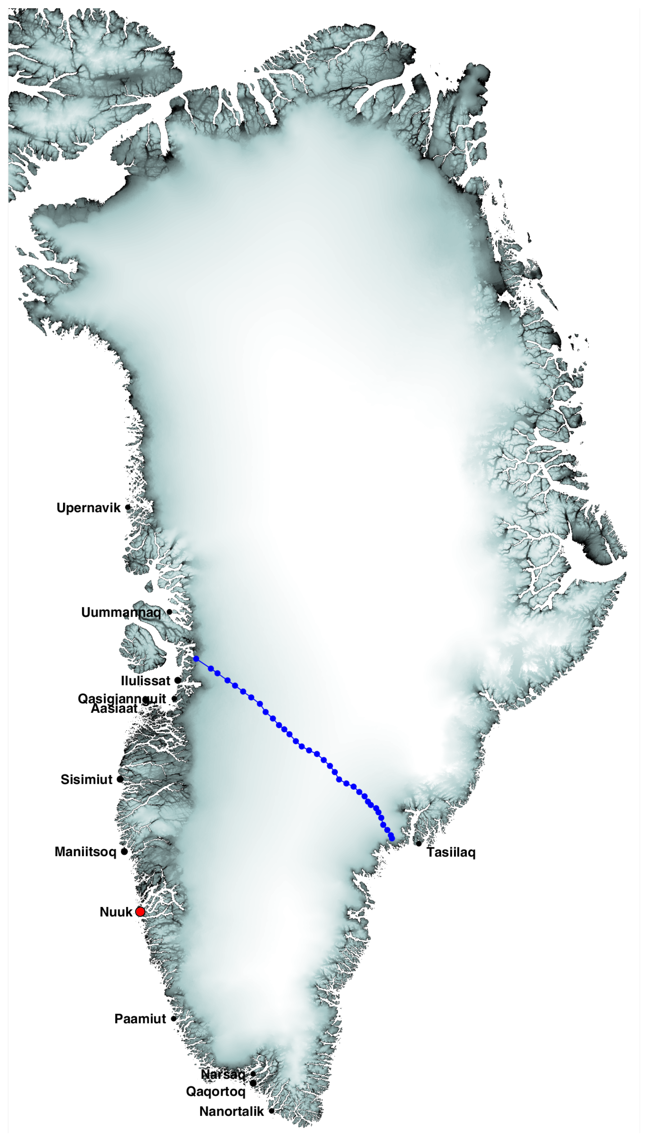
Figure 3 shows the surface topography of Greenland together with towns having more than 1000 inhabitants and the Greenland Korth Expeditions profile. The ice sheet covers around 80% of the surface of Greenland, and most settlements and towns are situated along the more accessible west coast.
In
Figure 4 the east–west Greenland Korth Expeditions route is shown together with campsite numbers. They have been defined during the first 2002 trek, but due to changing local conditions already the 2008 expedition did not repeat measurements at a first few sites (C1–C4) [
11]. In the next section, for comparing the GNSS data with altimetry, we will use a slightly reduced subset of the measurement sites; we used only the sites covering the full Greenland traverse where the complete time series of observations from the Greenland Korth Expeditions expeditions in 2002, 2006, 2010 and 2015 existed.
Figure 5 is a cross-section of Greenland along the Greenland Korth Expeditions profile. Although not to scale, it depicts clearly that during a 700 km long traverse from east to west, the Greenland Korth Expeditions team must climb up to the highest point of 2600 m (between sites No. 19 and 20) and descend afterwards. The majority of the measurement sites are located on a thick layer of snow and ice. The lowest point on the bed beneath the Greenland Korth Expeditions route corresponds to the location of Jakobshavn Glacier.
Figure 3,
Figure 4 and
Figure 5 make use of the BedMachine data for Greenland [
22,
23]. The currently available BedMachine (v3) is a self-consistent dataset of the Greenland ice sheet based on the conservation of mass; it includes the spatial grids for bed topography, surface elevation and ice thickness [
24]. The BedMachine dataset compiles radar-derived ice thickness measurements from 1993 to 2016 with a nominal date of 2007; the horizontal resolution of the bedrock topography and ice thickness is about 400 m.
In
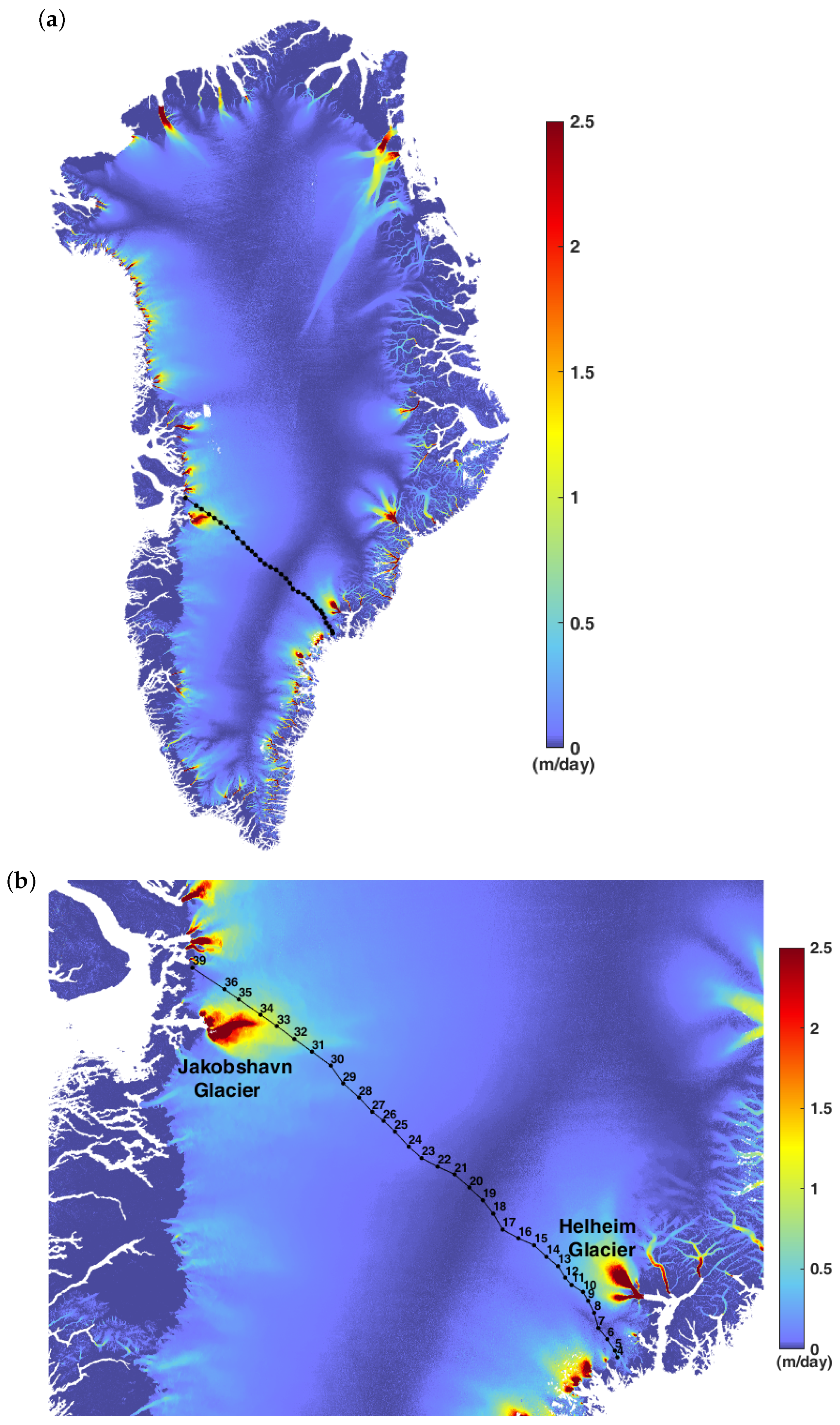
Figure 6, the Greenland Korth Expeditions profile is plotted on the ice velocity grid from synthetic aperture radar interferometry data of Sentinel-1 [
25]. The zero velocity areas dividing the ice sheet into several large drainage basins are clearly evident. In
Figure 6b we highlighted two large glaciers that are not far from the Greenland Korth Expeditions route, namely Helheim Glacier in the east and Jakobshavn Glacierin the west.
The data in
Figure 6 (and also in
Figure 7) were produced within the ESA Greenland ice sheet CCI project [
26].
4. Greenland Korth Expeditions and Satellite Altimetry
In this section we will compare the GNSS data measured along the Greenland Korth Expeditions profile (
Section 2) with satellite altimetry observations. Similarly to Korth et al. [
17] and Hofmann et al. [
20], at each measurement site three height differences were computed out of the Greenland Korth Expeditions height measurements in the years 2002, 2006, 2010 and 2015. For this study we selected only sites where measurements from all four campaings were available.
In
Figure 7a–c, the first three panels show maps of the surface elevation change from radar altimetry for 5 year periods corresponding to those defined by the GNSS data. The altimetry data were computed merging the observations from several satellites (ERS-1, ERS-2, Envisat, Cryosat-2, Sentinel-3) [
27,
28]. Already these maps demonstrate that the overall trend in the surface elevation loss is increasingly negative. During the period of 2002–2006, some areas in southern Greenland increased in elevation (see yellow shading,
Figure 7a), whereas for the 2010–2015 period, decreased surface elevations prevailed (see blue shading,
Figure 7c).
Figure 7d compares the surface elevation differences obtained from GNSS and satellite altimetry for the studied period of 2002–2015. Both datasets clearly show the same behavior, namely that with time one can observe larger drops in surface elevation. (This is not due to glacial isostatic adjustment as will be evident later in
Section 5). In the central part of the Greenland Korth Expeditions profile, at sites No. 11–28 (see
Figure 5b and
Figure 6b), there was an increase in surface elevations for the period of 2002–2006.
The largest drop in surface elevations took place at Greenland Korth Expeditions sites No. 31–35 near the western coast (
Figure 7d). This is the area of
Jakobshavn Glacier, one of the fastest moving glaciers in Greenland and Antarctica (
Figure 6b). Jakobshavn Glacier drains 6.5% of the Greenland ice sheet and produces around 10% of all Greenland icebergs [
29]. Based on satellite observations, the speed of Jakobshavn Glacier gradually increased from 5.7 km/yr to 12.6 km/yr over the period of 1992–2012. Surprisingly, over 2016–2018 Jakobshavn slowed to near its pre-1997 speed and is even thickening [
30]. One hypothesis for this behavior is that cooler ocean waters were advected to the glacier’s face in 2016, with water temperatures in the vicinity of Jakobshavn Glacier now colder than they have been since the mid-1980s [
30].
To assess the agreement between the GNSS and altimetry profiles,
Figure 7e compares the difference between GNSS and altimetry values from
Figure 7d with the uncertainty of the used satellite altimetry data. At the Greenland Korth Expeditions profile points, the accuracy of the ground-based GNSS measurements is higher than that of satellite altimetry, with a vertical measurement uncertainty of about ±3 cm [
11,
17].
Figure 7e confirms that the agreement of the GNSS and altimetry height differences is below the altimetry uncertainty curves in the majority of the measurement sites; larger discrepancies between GNSS and altimetry are found in the areas with large slopes (in the east, sites No. 5–11) and near Jakobshavn Glacier (sites No. 31–34), owing to slopes and considerable local ice dynamics.
We add a note on the Greenland Korth Expeditions sites in the context of the ice sheet surface properties and the slope. The current classification of the glacier zones (facies) distinguishes five basic types: dry snow, percolation, wet snow, superimposed ice and ablation zones [
31]. The majority of the Greenland Korth Expeditions measurement sites are located in the percolation zone, only a few peripheral sites (C5, C6, C35) are possibly located within the wet snow zone, and there is no Greenland Korth Expeditions site within the dry snow zone [
32,
33]. As for the slopes [
34], in the case of the Greenland Korth Expeditions measurement sites shown in
Figure 7d,e, all of the surface slopes are below 0.5
, except for site C5 with a slope of 1.2
and site C6 with a slope of 0.8
.
5. Greenland Korth Expeditions and Satellite Gravimetry
For comparing the GNSS profile differences over the period of 2002–2015, we will make use of satellite gravity data from the GRACE mission (Gravity Recovery And Climate Experiment; [
35]). During its 15-year flight (2002–2017), GRACE provided a time series of monthly gravity solutions with a resolution of 250–500 km at the Earth’s surface. These observations of global time-variable gravity have substantially contributed to various geoscientific domains, such as continental hydrological cycle, terrestrial water storage, solid earth changes due to large earthquakes, sea level monitoring, mass changes in polar ice sheets and large glaciers, and many others (for a review, see e.g., [
36,
37,
38]).
In our analyses, we will use one of the standard monthly GRACE gravity field solutions in the form of the spherical harmonic coefficients (UT CSR release 6, [
39]). In order to study the variations in the mass distribution of the water (snow, ice) storage near the Earth surface, satellite gravity measurements are expressed by means of the so-called
equivalent water height, which is directly connected to surface mass density (i.e., mass/area) [
9,
40,
41]. To suppress the errors in monthly gravity solutions that grow with harmonic degree (short scales, high-frequency noise), a Gaussian smoothing filter is usually applied; for Greenland we chose its radius to be 200 km (cf., [
42]).
In
Figure 8a–c, there are maps of the linear trend in the time series of GRACE monthly fields; the trend is expressed as the change in equivalent water height (cm/yr). They illustrate that the location of the maximum mass loss varied over this time period. Over the first Greenland Korth Expeditions period of 2002–2006, Greenland’s mass loss was concentrated in the south-east part of the island (
Figure 8a). During the second Greenland Korth Expeditions period of 2006–2010, the maximum mass loss migrated to the central west coast of Greenland (
Figure 8b). Finally, the dominant mass loss location shifted southward during the third Greenland Korth Expeditions period of 2010–2015 (
Figure 8c). This agrees with other observations [
6]. Within the currently available record of Greenland’s satellite observations in 1992–2019, satellite gravimetry estimates the maximum mass loss rate in Greenland to have taken place in 2011, followed by an extreme summertime surface melting in 2012 [
6].
Next, the GNSS observations reported here are compared to GRACE along the Greenland Korth Expeditions profile. As mentioned in the Introduction, there are several differences between local and satellite observations. The GNSS data are obtained locally, but GRACE integrates the mass variations over an area of about 300 km in diameter. The GNSS vertical component measures the variation in height, while GRACE observes the mass changes. Finally, one must decide on the use of glacial isostatic adjustment model to get the net change in height or mass, corrected for the Earth’s crust uplift.
In
Figure 8d we show the correction due to glacial isostatic adjustment (GIA) for Greenland. It is one of the standard GIA models, giving constant time rates for compressible Earth, computed using the ICE-5G ice history and the VM2 viscosity profile [
43,
44]. The figure shows that there is only a small change in the altitudes due to GIA over the Greenland Korth Expeditions profile; in Greenland the crust is modeled to rise somewhat only in the north. We will use this GIA correction for net mass balance estimates in the next section, while in this section we will not correct GRACE for GIA.
Another point to consider is different spatial averaging of ground-based GNSS and GRACE observations (e.g., [
45]). Here we applied the Gaussian smoothing filter of the same radius of 200 km to the GNSS data [
40,
41].
In
Figure 8e, on the yearly averaged time series of GRACE monthly solutions we superimposed the GNSS elevation differences obtained at one of the Greenland Korth Expeditions sites (shown as a red point in
Figure 8a–c). This particular site, No. 26, is located in the central part of the profile, at an altitude of 2270 m (
Figure 5). In order to convert the altitude changes into mass changes one needs some model of the firn density; due to changing physical conditions (especially temperature), in these models there is a large uncertainty. Here, as the firn density we used a rather conservative estimate of 600 ± 300 kg m
for Greenland regions above 2000 m [
46]. As is shown in
Figure 8e, three GNSS height differences agree well with GRACE mass estimates within the uncertainty limits (shown as transparent error bars). Let us also point to the correspondence between the three GNSS steps in panel
Figure 8e of gradually increasing size and the trend values (indicated by different colors) at the measurement site in three panels of
Figure 8a–c.
There are several reasons to show the comparison between the GNSS and GRACE datasets for only one illustrative location. As mentioned at the end of the previous section, virtually all Greenland Korth Expeditions sites are located in the percolation zone of the ice sheet, except for a very few endpoints. Then, to compare the point-wise GNSS data with the much lower-resolution GRACE data, we applied the 200-km Gaussian smoothing to the GNSS profile. As a result, the local features along the GNSS profile are smeared and combined together. Finally, for a comparison between such an averaged GNSS profile and GRACE monthly gravity fields, a typical point near the middle of the traverse was selected, for which the GRACE trend maps in
Figure 8a–c display a different value in each period.
5.1. Mass Balance for Southern Greenland (2002–2006)
For the first difference period of the Greenland Korth Expeditions, of 2002–2006, we estimated the mass loss rate for southern Greenland, defined by Korth et al. [
11] to be roughly the area of Greenland south of the Greenland Korth Expeditions profile. Based on GRACE gravity data, we obtained the value of −68 ± 11 Gt/yr, which compares very well with the value of −70 Gt/yr estimated by Korth et al. [
11].
The method used for the mass rate estimate from GRACE data for southern Greenland is described in the next section, where it is applied to the entire Greenland ice sheet.
6. Updated Estimate of Mass Change in the Greenland Ice Sheet from Satellite Gravimetry
The GRACE satellites started observing the Earth’s gravity field in 2002, and during the first few years in orbit the GRACE measurements of the time-variable gravity were validated by independent terrestrial, mainly seasonal hydrological data [
35,
47,
48], and only afterwards first estimates of Antarctic and Greenland mass loss based on estimated linear trend started to appear [
49,
50,
51,
52].
In
Figure 9a–d we present maps for the linear trend fitted to the time series of GRACE monthly fields. The results in this section are derived from monthly gravity solutions corrected for the glacial isostatic adjustment effect (
Section 5). The particular displayed periods were selected to highlight the changing location of the maximum mass loss over time. Over 2002–2007 the maximum of the mass loss stayed in south-east Greenland, and then it moved to the entire west coast and peaked over 2007–2012. In the final years of GRACE in orbit, 2012–2017, the maximum mass loss was confined to the central west. These three approximately homogeneous phases produce an average trend map shown in
Figure 9d.
In
Figure 10 we present the time evolution of mass balance for the Greenland ice sheet derived from satellite observations. As a reference, we show the reconciled estimate of the Greenland mass rate from the Ice Sheet Mass Balance Inter-Comparison Exercise (IMBIE), a collaboration between scientists supported by ESA and NASA [
53]. The IMBIE-2019 ice sheet mass balance estimate (in blue) is based on 26 individual groups of satellite measurements coming from altimetry, gravimetry and the input–output method [
6,
8]. The longest record starting in 1992 is derived from the input–output method, which is based on estimating the balance between input (surface mass balance of snowfall, rainfall vs. sublimation, runoff) and output (ocean ice discharge).
Figure 10 shows a balanced mass budget until around 2002, when a mass loss started to prevail.
Monthly gravity fields from GRACE are available for its 15-year operational period covering 4/2002–6/2017. In order to proceed with successful GRACE observations, a continuation mission GRACE Follow-On (GRACE-FO) was organized and has started to provide monthly solutions since 6/2018 [
54,
55].
Due to technical problems with launching the two GRACE-FO satellites, a one-year gap in the time series of monthly gravity fields produced by GRACE and GRACE-FO occurred. This one-year gap may be completed by gravity fields derived from the GNSS tracking of three Swarm satellites, in low-Earth orbit since 11/2013 [
56,
57]. Indeed, it was demonstrated that precise satellite positions from the geodetic-quality GNSS receivers (one receiver aboard each Swarm satellite) could be processed to produce monthly gravity fields that, although with a reduced spatial resolution of 1300 km and more noise, are able to produce reasonable estimates also for the mass trends in Greenland [
58,
59,
60,
61].
We processed the monthly gravity solutions of GRACE, GRACE-FO and Swarm similarly to the IMBIE approach; the linear trend was fitted within a 36-month moving window using a weighted least squares [
6]. To reduce the higher noise in the Swarm monthly gravity fields, for computing the linear trend we used a 48-month moving window.
As shown in
Figure 10, our GRACE estimated mass loss rates (in red) accompanied with an uncertainty band agree well with the reference IMBIE-19 curve. In accordance with other gravimetry solutions shown in the IMBIE-19 paper [
6], the maximum yearly mass loss from GRACE was recorded in 2011, followed by a return to moderate mass balance values over 2012–2017. Towards the end of the GRACE mission in 2017, as a consequence of a lower number of monthly fields used in the fit, the estimated uncertainty band of GRACE started to widen to some extent. This is the case also for GRACE-FO, for which so far only a limited number of monthly solutions is available (6/2018–9/2020). In the last period covering 2018–2019, the estimated trend from GRACE-FO observations seems to indicate an increased mass loss again. This conclusion is supported by the Swarm trend estimates (in green).
Finally, based on the obtained yearly trend values, in
Table 2 we present average mass trends over the previously described periods, where the Greenland mass balance displayed some overall characteristic features (
Figure 9a–c).
7. Conclusions
The objective of this paper was to present the Greenland Korth Expeditions in relation to satellite observations and to connect satellite data to some of the Greenland Korth Expeditions scientific results, namely to the unique time series of the GNSS data measured on a periodic basis (2002, 2006, 2010, 2015) at the same sites along the 700-km traverse across Greenland. In
Section 3 we displayed the Greenland Korth Expeditions profile and individual measurement sites on the background of surface and bed topography maps. A projection on the map of the ice velocity distribution across Greenland precisely localizes the measurement sites with respect to the underlying ice speed. A special feature of the Greenland Korth Expeditions profile is the closeness of its several sites to the important Jakobshavn Glacier in the west of Greenland. This plays a role in
Section 4, where the vertical component of the GNSS data from the Greenland Korth Expeditions profile is compared to heights observed by satellite radar altimetry. We demonstrated a very good overall agreement between GNSS and altimetry, although there are some differences near the ice sheet margins. These are due to the limited accuracy of satellite altimetry in regions with slopes, and also to the rather variable ice dynamics in the area of Jakobshavn Glacier.
Section 5 deals with comparing the GNSS data with satellite gravimetry as given by GRACE monthly gravity fields. By processing both the GNSS and GRACE datasets to be comparable, we showed their agreement for the time series of surface density at one of the Greenland Korth Expeditions measurement sites. In
Section 5.1, using our satellite gravimetry computation, we independently confirmed the previous estimate by Korth et al. [
11] for the yearly mass change in southern Greenland derived from the Greenland Korth Expeditions profile over 2002–2006. Following the same method, but applied to the Greenland ice sheet as a whole,
Section 6 provides an updated estimate of the Greenland mass balance based on satellite gravimetry from the GRACE, GRACE-FO and Swarm missions. Over the GRACE mission period covering 2002–2015, our estimates are in accordance with the IMBIE project results used as a reference. [Agreement at the level of the uncertainty bands for both datasets is shown in
Figure 10]. For the latest time interval of 2018–2019, our estimate combining GRACE-FO and Swarm data indicates a renewal of a more intensified mass loss in Greenland.


