Mobile Robot Path Optimization Technique Based on Reinforcement Learning Algorithm in Warehouse Environment

Abstract

This paper reports on the use of reinforcement learning technology for optimizing mobile robot paths in a warehouse environment with automated logistics. First, we compared the results of experiments conducted using two basic algorithms to identify the fundamentals required for planning the path of a mobile robot and utilizing reinforcement learning techniques for path optimization. The algorithms were tested using a path optimization simulation of a mobile robot in same experimental environment and conditions. Thereafter, we attempted to improve the previous experiment and conducted additional experiments to confirm the improvement. The experimental results helped us understand the characteristics and differences in the reinforcement learning algorithm. The findings of this study will facilitate our understanding of the basic concepts of reinforcement learning for further studies on more complex and realistic path optimization algorithm development.

1. Introduction

The fourth industrial revolution and digital innovation have led to the increased interest in the use of robots across industries; thus, robots are being used in various industrial sites. Robots can be broadly categorized as industrial or service robots. Industrial robots are automated equipment and machines used in industrial sites such as factory lines and are used for assembly, machining, inspection, and measurement as well as pressing and welding [1]. The use of service robots is expanding in manufacturing environments and other areas such as industrial sites, homes, and institutions. Service robots can be broadly divided into personal service robots and professional service robots. In particular, professional service robots are robots used by workers to perform tasks, and mobile robots are one of the professional service robots [2].

A mobile robot needs the following elements to perform tasks: localization, mapping, and path planning. First, the location of the robot must be known in relation to the surrounding environment. Second, a map is needed to identify the environment and move accordingly. Third, path planning is necessary to find the best path to perform a given task [3]. Path planning has two types: point-to-point and complete coverage. A complete coverage path planning is performed when all positions must be checked, such as for a cleaning robot. A point-to-point path planning is performed for moving from the start position to the target position [4].

To review the use of reinforcement learning as a path optimization technique for mobile robots in a warehouse environment, the following points must be understood. First, it is necessary to understand the warehouse environment and the movement of mobile robots. To do this, we must check the configuration and layout of the warehouse in which the mobile robot is used as well as the tasks and actions that the mobile robot performs in this environment. Second, it is necessary to understand the recommended research steps for the path planning and optimization of mobile robots. Third, it is necessary to understand the connections between layers and modules as well as their working when they are integrated with mobile robots, environments, hardware, and software. With this basic information, a simulation program for real experiments can be implemented. Because reinforcement learning can be tested only when a specific experimental environment is prepared in advance, substantial preparation of the environment is required early in the study but the researcher must prepare it. Subsequently, the reinforcement learning algorithm to be tested is integrated with the simulation environment for the experiment.

This paper discusses an experiment performed using a reinforcement learning algorithm as a path optimization technique in a warehouse environment. Section 2 briefly describes the warehouse environment, the concept of path planning for mobile robots, the concept of reinforcement learning, and the algorithms to be tested. Section 3 briefly describes the structure of the mobile robot path-optimization system, the main logic of path search, and the idea of dynamically adjusting the reward value according to the moving action. Section 4 describes the construction of the simulation environment for the experiments, the parameters and reward values to be used for the experiments, and the experimental results. Section 5 presents the conclusions and directions for future research.

2. Related Work

2.1. Warehouse Environment

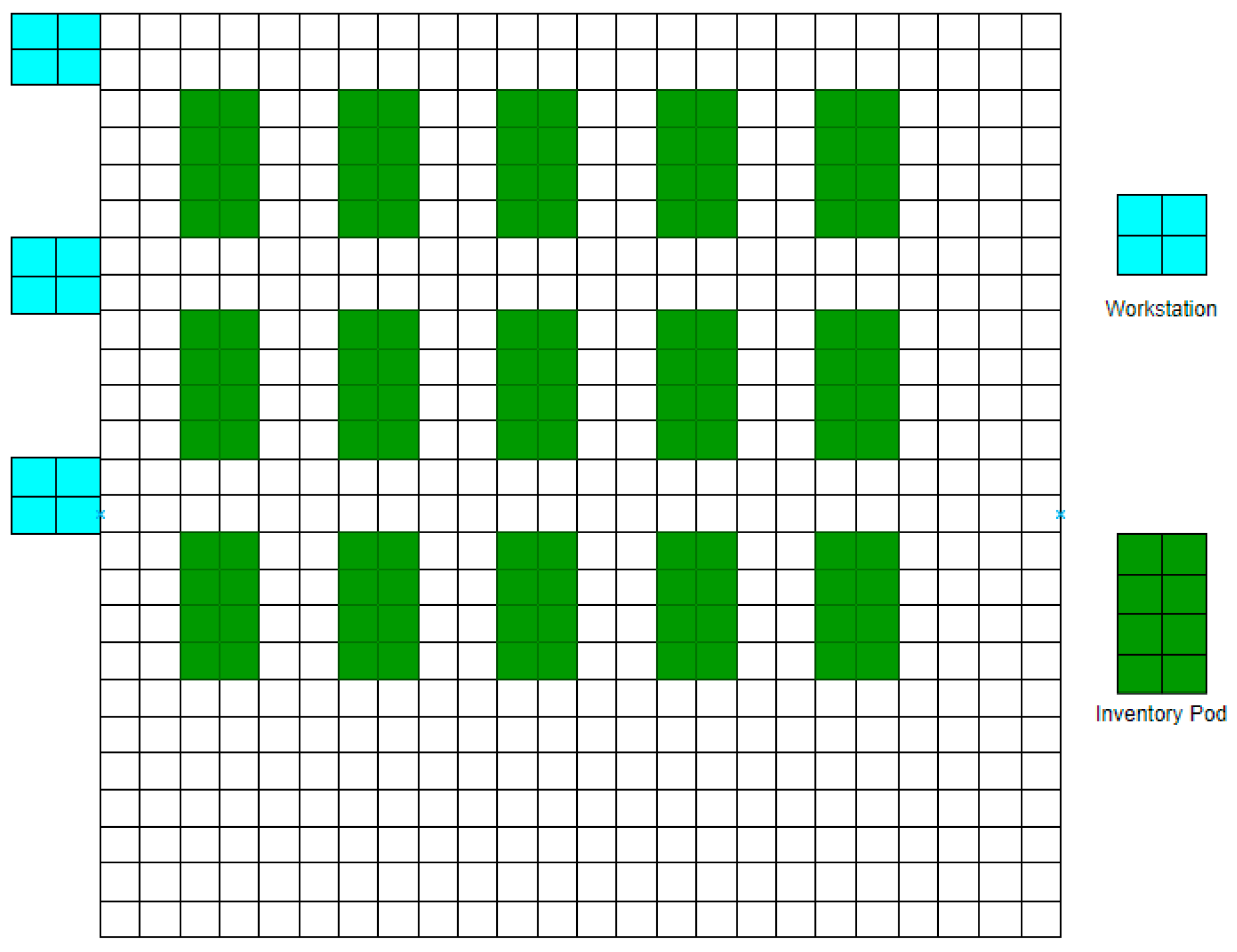
2.1.1. Warehouse Layout and Components

The major components for automated warehouse with mobile robots are as follows [5,6,7,8,9,10].

• Robot drive device: It instructs the robot from the center to pick or load goods between the workstation and the inventory pod.
• Inventory pod: This is a shelf rack that includes storage boxes. There are two standard sizes: a small pod can hold up to 450 kg, and a large pod can load up to 1300 kg.
• Workstation: This is the work area in which the worker operates and performs tasks such as replenishment, picking, and packaging.

Figure 1 shows an example of a warehouse layout with inventory pods and workstations.

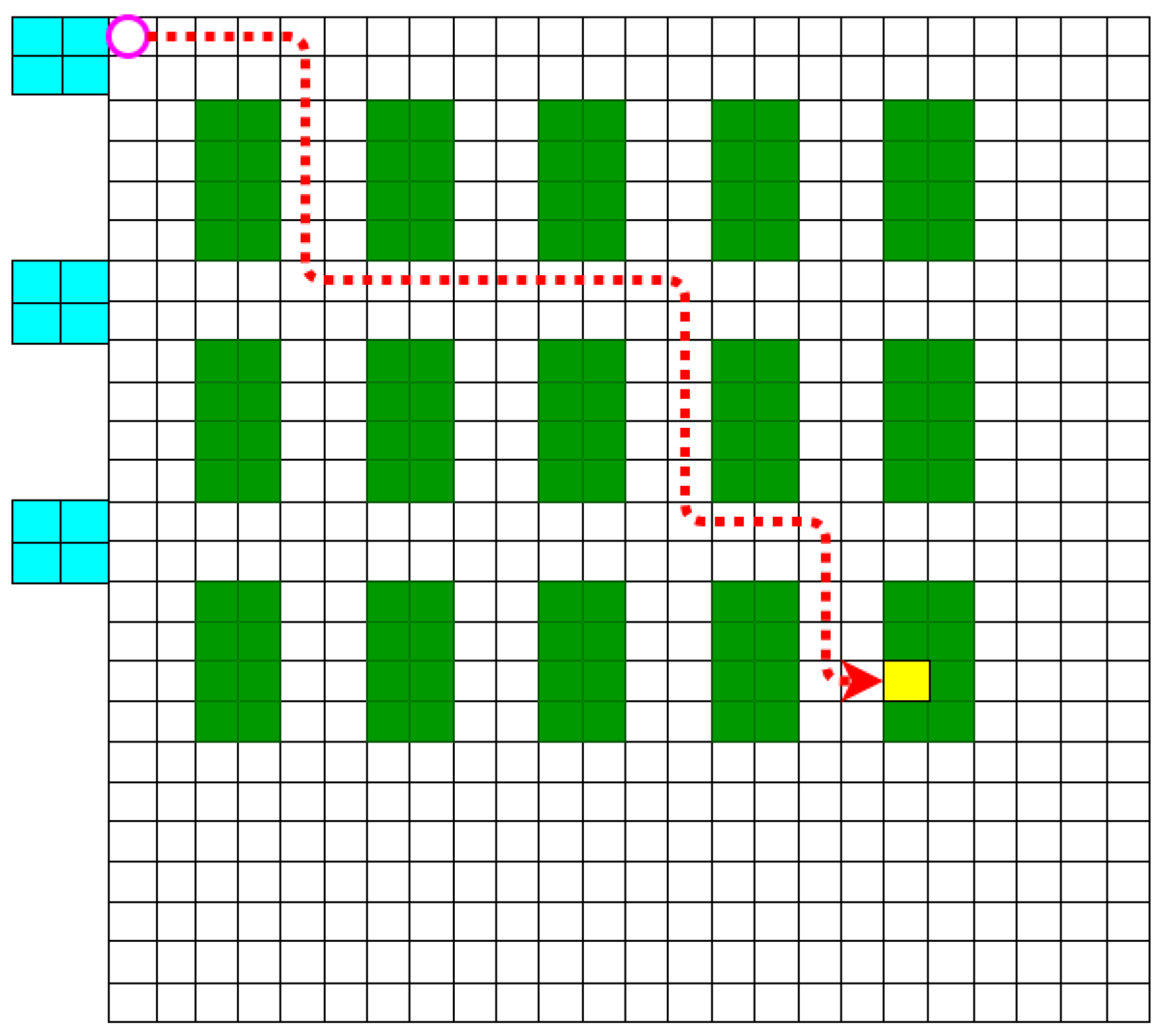
2.1.2. Mobile Robot’s Movement Type

In the robotic mobile fulfillment system, a robot performs a storage trip, in which it transports goods, and a retrieval trip, in which it moves to pick up goods. After dropping the goods into the inventory pod, additional goods can be picked up or returned to the workstation [11].

The main movements of the mobile robot in the warehouse are to perform the following tasks [12].

• move goods from the workstation to the inventory pod;
• move from one inventory pod to another to pick up goods;
• move goods from the inventory pod to the workstation

2.2. Path Planning for Mobile Robot

For path planning in a given work environment, a mobile robot searches for an optimal path from the starting point to the target point according to specific performance criteria. In general, path planning is performed for two path types, global and local, depending on whether the mobile robot has environmental information. In the case of global path planning, all information about the environment is provided to the mobile robot before it starts moving. Based on local path planning, the robot does not know most information about the environment before it moves [13,14].

The path planning development process for mobile robots usually follows the steps below in Figure 2 [13].

• Environmental modeling
• Optimization criteria
• Path finding algorithm

The classification of the path planning of the mobile robot is illustrated in Figure 3.

Dijkstra, A*, and D* algorithms for the heuristic method are the most commonly used algorithms for path search in global path planning [13,15]. Traditionally, warehouse path planning has been optimized using heuristics and meta heuristics. Most of these methods work without additional learning and require significant computation time as the problem becomes complex. In addition, it is challenging to design and understand heuristic algorithms, making it difficult to maintain and scale the path. Therefore, interest in artificial intelligence technology for path planning is increasing [16].

2.3. Reinforcement Learning Algorithm

Reinforcement learning is a method that uses trial and error to find a policy to reach a goal by learning through failure and reward. Deep neural networks learn weights and biases from labeled data, and reinforcement learning learns weights and biases using the concept of rewards [17].

The essential elements of reinforcement learning are as follows, and see Figure 4 for how to interact.

First, agents are the subjects of learning and decision making. Second, the environment refers to the external world recognized by the agent and interacts with the agent. Third is policy. The agent finds actions to be performed from the state of the surrounding environment. The fourth element is a reward, an information that tells you if an agent has done good or bad behavior. In reinforcement learning, positive rewards are given for actions that help agents reach their goals, and negative rewards are given for actions that prevent them from reaching their goals. The fifth element is a value function. The value function tells you what’s good in the long term. Value is the total amount of reward an agent can expect. Sixth is the environmental model. Environmental models predicts the next state and the reward that changes according to the current state. Planning is a way to decide what to do before experiencing future situations. Reinforcement learning using models and plans is called a model-based method, and reinforcement learning using trial and error is called a model free method [18].

The basic concept of reinforcement learning modeling aims to find the optimal policy for problem solving and can be defined on the basis of the Markov Decision Process (MDP). If the state and action pair is finite, this is called a finite MDP [18]. The most basic Markov process concept in MDP, consists of a state s, a state transition probability p, and an action a performed. The p is the probability that when performing an action a in state s, it will change to s’ [18].

The Formula (1) that defines the relationship between state, action and probability is as follows [18,19].

$$p\left(s^{\prime }\mid s,a\right)= \mathrm{Pr}\left\{S_t=s^{\prime }\mid S_{t-1}=s,A_{t-1}=a\right\}$$

(1)

The agent’s goal is to maximize the sum of regularly accumulated rewards, and the expected return is the sum of rewards. In other words, using rewards to formalize the concept of a goal is characteristic of reinforcement learning. In addition, the discount factor is also important in the concept of reinforcement learning. The discount factor (γ) is a coefficient that discounts the future expected reward and has a value between 0 and 1 [18]. Discounted return obtained through reward and depreciation rate can be defined as the following Formula (2) [18,19].

$$G_t=R_{t+1}+\gamma R_{t+2}+{\gamma }^2{R}_{t+3}+\cdots ={\displaystyle \sum }_{k=0}^{\infty }{\gamma }^k{R}_{t+k+1}$$

(2)

The reinforcement learning algorithm has the concept of a value function, a function of a state that estimates whether the environment given to an agent is good or bad. Moreover, the value function is defined according to the behavioral method called policy. Policy is the probability of choosing possible actions in a state [18].

If the value function was the consideration of the cumulative reward and the change of state together, the state value function was also considered the policy [20]. The value function is the expected value of the return if policy π is followed since starting at state s, and the formulas are as follows [18,20].

$$v_{\pi }\left(s\right)={\mathbb{E}}_{\pi }\left[G_t\mid S_t=s\right]={\mathbb{E}}_{\pi }\left[{\displaystyle \sum }_{k=0}^{\infty }{\gamma }^k{R}_{t+k+1}\mid S_t=s\right]$$

(3)

Among the policies, the policy with the highest expected value of return is the optimal policy, and the optimal policy has an optimal state value function and an optimal action value function [18]. The optimal state value function can be found in equation (4), and the optimal action value function can be found in Equations (5) and (6) [18,20].

$$v_{*}\left(s\right)=\underset{\pi }{max}{v}_{\pi }\left(s\right)$$

(4)

$$q_{*}\left(s,a\right)=\underset{\pi }{max}{q}_{\pi }\left(s,a\right)$$

(5)

$$= \mathbb{E}\left[R_{t+1}+\gamma v_{*}\left(S_{t+1}\right)\mid S_t=s,A_t=a\right]$$

(6)

The value of a state that follows an optimal policy is equal to the expected value of the return from the best action that can be chosen in that state [18]. The formula is as follows [18,20].

$$q_{*}\left(s,a\right)=\mathbb{E}\left[R_{t+1}+\gamma \underset{a^{\prime }}{max}{q}_{*}\left(S_{t+1},a^{\prime }\right)\mid S_t=s,A_t=a\right]$$

(7)

$$={\displaystyle \sum }_{s^{\prime },r}p\left(s^{\prime },r\mid s,a\right)\left[r+\gamma \underset{a^{\prime }}{max}{q}_{*}\left(s^{\prime },a^{\prime }\right)\right]$$

(8)

2.3.1. Q-Learning

One of most basic algorithm among reinforcement learning algorithms is off-policy temporal-difference control algorithm known as Q-Learning [18]. The Q-Learning algorithm stores the state and action in the Q Table in the form of a Q Value; for action selection, it selects a random value or a maximum value according to the epsilon-greedy value and stores the reward values in the Q Table [18].

The algorithm stores the values in the Q Table using Equation (9) below [21].

$$Q\left(s,a\right)=r\left(s,a\right)+\underset{a}{max}\left(Q\left(s^{\prime },a\right)\right)$$

(9)

Equation (9) is generally converted into update—Equation (10) by considering a factor of time [18,22,23].

$$Q\left(s,a\right)\leftarrow Q\left(s,a\right)+\alpha \left(r+\gamma \underset{a^{\prime }}{max}Q\left(s^{\prime },a^{\prime }\right)-Q\left(s,a\right)\right)$$

(10)

The procedure of the Q-Learning algorithm is as follows (Algorithm 1) [18].

Algorithm 1: Q-Learning.

Initialize Q(s, a)

Loop for each episode:

Initialize s (state)

Loop for each step of episode until s (state) is destination:

Choose a (action) from s (state) using policy from Q values

Take a (action), find r (reward), s’ (next state)

Calculate Q value and Save it into Q Table

Change s’ (next state) to s (state)

In reinforcement learning algorithms, the process of exploration and exploitation plays an important role. Initially, lower priority actions should be selected to investigate the best possible environment, and then select and proceed with higher priority actions [23]. The Q-Learning algorithm has become the basis of the reinforcement learning algorithm because it is simple and shows excellent learning ability in a single agent environment. However, Q-Learning updates only once per action; it is thus difficult to solve complex problems effectively when many states and actions have not yet been realized.

In addition, because the Q table for reward values is predefined, a considerable amount of storage memory is required. For this reason, the Q-Learning algorithm is disadvantageous in a complex and advanced multi-agent environment [24].

2.3.2. Dyna-Q

Dyna-Q is a combination of the Q-Learning and Q-Planning algorithms. The Q-Learning algorithm changes a policy based on a real experience. The Q-Planning algorithm obtains simulated experience through search control and changes the policy based on a simulated experience [18]. Figure 5 illustrates the structure of the Dyna-Q model.

The Q-Planning algorithm randomly selects samples only from previously experienced information, and the Dyna-Q model obtains information for simulated experience through search control exactly as it obtains information through modeling learning based on a real experience [18]. The Dyna-Q update-equation is the same as that for Q-Learning (10) [22].

The Dyna-Q algorithm is as follows (Algorithm 2) [18].

Algorithm 2: Dyna-Q.

Initialize Q(s, a)

Loop forever:

(a) Get s (state)

(b) Choose a (action) from s (state) using policy from Q values

(c) Take a (action), find r (reward), s’ (next state)

(d) Calculate Q value and Save it into Q Table

(e) Save s (state), a (action), r (reward), s’ (next state) in memory

(f) Loop for n times

Take s(state), a (action), r (reward), s’ (next state)

Calculate Q value and Save it into Q Table

(g) Change s’ (next state) to s (state)

Steps (a) to (d) and, (g) are the same as in Q-Learning. Steps (e) and (f) added to the Dyna-Q algorithm store past experiences in memory to generate the next state and a more accurate reward value.

3. Reinforcement Learning-Based Mobile Robot Path Optimization

3.1. System Structure

In the mobile robot framework structure in Figure 6, the agent is controlled by the supervisor controller, and the robot controller is executed by the agent, so that the robot operates in the warehouse environment and the necessary information is observed and collected [25,26,27].

3.2. Operation Procedure

The mobile robot framework works as follows. At the beginning, the simulator is set to its initial state, and the mobile robot collects the first observation information and sends it to the supervisor controller. The supervisor controller verifies the received information and communicates the necessary action to the agent. At this stage, the supervisor controller can obtain additional information if necessary. The supervisor controller can communicate job information to the agent. The agent conveys the action to the mobile robot through the robot controller, and the mobile robot performs the received action using actuators. After the action is performed by the robot controller, the changed position and status information is transmitted to the agent and the supervisor controller, and the supervisor controller calculates the reward value for the performed action. Subsequently, the action, reward value, and status information are stored in memory. These procedures are repeated until the mobile robot achieves the defined goal or the number of epochs/episodes or conditions that satisfy the goal [25].

In Figure 7, we show an example class that is composed of the essential functions and main logic required by the supervisor controller for path planning.

3.3. Dynamic Reward Adjustment Based on Action

The simplest type of reward for the movement of a mobile robot in a grid-type warehouse environment is achieved by specifying a negative reward value for an obstacle and a positive reward value for the target location. The direction of the mobile robot is determined by its current and target positions. The path planning algorithm requires significant time to find the best path by repeating many random path finding attempts. In the case of the basic reward method introduced earlier, an agent searches randomly for a path, regardless of whether it is located far from or close to the target position. To improve on these vulnerabilities, we considered a reward method as shown in Figure 8.

The suggestions are as follows:

First, when the travel path and target position are determined, a partial area close to the target position is selected. (Reward adjustment area close to the target position).

Second, a higher reward value than the basic reward method is assigned to the path positions within the area selected in the previous step. Third, we propose a method to select an area as above whenever the movement path changes and changes the position of the movement path in the selected area to a high reward value. This is called dynamic reward adjustment based on action, and the following (Algorithm 3) is an algorithm of the process.

Algorithm 3: Dynamic reward adjustment based on action.

1. Get new destination to move

2. Select a partial area near the target position.

3. A higher positive reward value is assigned to the selected area, excluding the target point and obstacles.

(Highest positive reward value to target position)

4. Test and Results

4.1. Warehouse Simulation Environment

To create a simulation environment, we referred to the paper [23] and built a virtual experiment environment based on the previously described warehouse environment. A total of 15 inventory pods were included in a 25 × 25 grid layout. A storage trip of a mobile robot from the workstation to the inventory pod was simulated. This experiment was conducted to find the optimal path to the target position, avoiding inventory pods at the starting position where a single mobile robot was defined.

The Figure 9 shows the target position for the experiments.

4.2. Test Parameter Values

Q-Learning and Dyna-Q algorithms were tested in a simulation environment.

Table 1. Parameter values for experiment.

Parameter	Q-Learning	Dyna-Q
Learning Rate (α)	0.01	0.01
Discount Rate (γ)	0.9	0.9

shows the parameter values used in the experiment.

4.3. Test Reward Values

The experiment was conducted with the following reward methods.

• Basic method: The obstacle was set as −1, the target position as 1, and the other positions as 0.
• Dynamic reward adjustment based on action: To check the efficacy of the proposal, an experiment was conducted designating set values that were similar to those in the proposed method as shown in Figure 10 [28,29,30]. The obstacle was set as −1, the target position as 10, the positions in the selected area (area close to target) as 0.3, and the other positions as 0.

4.4. Results

First, we tested two basic reinforcement learning algorithms: the Q-Learning algorithm and the Dyna-Q algorithm. The experiment was performed five times for each algorithm, and there may be deviations in the results for each experiment, so the experiment was performed under the same condition and environment. The following points were verified and compared using the experimental results. The optimization efficiency of each algorithm was checked based on the length of the final path, and the path optimization performance was confirmed by the path search time. We were also able to identify learning patterns by the number of learning steps per episode.

The path search time of the Q-Learning algorithm was 19.18 min for the first test, 18.17 min for the second test, 24.28 min for the third test, 33.92 min for the fourth test, and 19.91 min for the fifth test. It took about 23.09 min on average. The path search time of the Dyna-Q algorithm was 90.35 min for the first test, 108.04 min for the second test, 93.01 min for the third test, 100.79 min for the fourth test, and 81.99 min for the fifth test. The overall average took about 94.83 min.

The final path length of the Q-Learning algorithm was 65 steps for the first test, 34 steps for the second test, 60 steps for the third test, 91 steps for the fourth test, 49 steps for the fifth test, and the average was 59.8 steps. The final path length of the Dyna-Q algorithm was 38 steps for the first test, 38 steps for the second test, 38 steps for the third test, 34 steps for the fourth test, 38 steps for the fifth test, and the average was 37.2 steps.

The Q-Learning algorithm was faster than Dyna-Q in terms of path search time, and Dyna-Q selected shorter and simpler final paths than those selected by Q-Learning. Figure 11 and Figure 12 show the learning pattern through the number of training steps per episode. Q-Learning found the path by repeating many steps for 5000 episodes. Dyna-Q, stabilized after finding the optimal path between 1500 and 3000 episodes. In both algorithms, the maximum number of steps rarely exceeded 800 steps. All tests ran 5000 episodes for each test. In the case of Q-Learning algorithm, the second test exceeded 800 steps 5 times (0.1%) and fourth test exceeded 800 steps 5 times (0.1%). So, Q-Learning algorithm test exceeded 800 steps at a total level of 0.04% in the five tests. In the case of Dyna-Q algorithm, the first test exceeded 800 steps once (0.02%), third test exceeded 800 steps 7 times (0.14%), fifth test exceeded 800 steps 3 times (0.06%). So, Dyna-Q algorithm test exceeded 800 steps at a total level of 0.044 % in the five tests. To compare the path search time and the learning pattern result, we compared the experiment (e) of the two algorithms. The path search time was 19.9 s for Q-Learning algorithm and 81.98 s for Dyna-Q. Looking at the learning patterns in Figure 11 and Figure 12, the Q-Learning algorithm learned by executing 200 steps to 800 steps per each episode until the end of 5000 episodes, and the Dyna-Q algorithm learned by executing 200 steps to 800 steps per each episode until the middle of the 2000 episode. However, the time required for the Dyna-Q algorithm is more than 75% slower than the Q-Learning algorithm. In this perspective, it has been confirmed that Dyna-Q takes longer to learn in a single episode than Q-Learning.

Subsequently, additional experiments were conducted by applying ‘dynamic reward adjustment based on action’ to the Q-Learning algorithm. The path search time of this experiment was 19.04 min for the first test, 15.21 min for the second test, 17.05 min for the third test, 17.51 min for the fourth test, and 17.38 min for the fifth test. It took about 17.23 min on average. The final path length of this experiment was 38 steps for the first test, 34 steps for the second test, 34 steps for the third test, 34 steps for the fourth test, and 34 steps for the fifth test. The average was 34.8 steps. The experimental results can be seen in Figure 13, and it includes the experimental results of Q-Learning and Dyna-Q previously conducted. In the case of the Q-Learning algorithm to which ‘dynamic reward adjustment based on action’ was applied, the path search time was slightly faster than Q-Learning, and the final path length was confirmed to be improved to a level similar to that of Dyna-Q. Figure 14 shows the learning pattern obtained using the additional experiments compared with the result of Q-Learning. There is no outstanding point. Figure 15 shows the path found through the experiment of the Q Leaning algorithm applying ‘dynamic reward adjustment based on action’ on the map.

5. Conclusions

In this paper, we reviewed the use of reinforcement learning as a path optimization technique in a warehouse environment. We built a simulation environment to test path navigation in a warehouse environment and tested the two most basic algorithms, the Q-Learning and Dyna-Q algorithms, for reinforcement learning. We then compared the experimental results in terms of the path search times and the final path lengths. Compared with the average of the results of the five experiments, the path search time of the Q-Learning algorithm was about 4.1 times faster than the Dyna-Q algorithm’s, and the final path length of Dyna-Q algorithm was about 37% shorter than the Q-Learning algorithm’s. As a result, the experimental results of both Q-Learning and Dyna-Q algorithm showed unsatisfactory results for either the path search time or the final path length. To improve the results, we conducted various experiments using the Q-Learning algorithm and found that it does not perform well when finding search paths in a complex environment with many obstacles. The Q-Leaning algorithm has the property of finding a path at random. To minimize this random path searching trial, the target position was determined for movement, and the set reward value was high around the target position,’ thus the performance and efficiency of the agent improved with ‘dynamic reward adjustment based on action’. Agents mainly explore locations with high reward values. In further experiments, the path search time was about 5.5 times faster than the Dyna-Q algorithm’s, and the final path length was about 71% shorter than the Q-Learning algorithm. It was confirmed that the path search time was slightly faster than the Q-Learning algorithm, and the final path length was improved to the same level as the Dyna-Q algorithm.

It is a difficult goal to meet both minimization of path search time and high accuracy for path search. If the learning speed is too fast, it will not converge to the optimal value function, and if the learning speed is set too late, the learning may take too long. In this paper, we have experimentally confirmed how to reduce inefficient exploration with simple technique to improve path search accuracy and maintain path search time.

In this study, we have seen how to use reinforcement learning for a single agent and a path optimization technique for a single path, but the warehouse environment in the field is much more complex and dynamically changing. In the automation warehouse, multiple mobile robots work simultaneously. Therefore, this basic study is an example of improving the basic algorithm in a single path condition for a single agent, and it is insufficient to apply the algorithm to an actual warehouse environment. Therefore, based on the obtained results, an in-depth study of the improved reinforcement learning algorithm is needed, considering highly challenging multi-agent environments to solve more complex and realistic problems.

References

1. Hajduk, M.; Koukolová, L. Trends in Industrial and Service Robot Application. Appl. Mech. Mater. 2015, 791, 161–165. [Google Scholar] [CrossRef]
2. Belanche, D.; Casaló, L.V.; Flavián, C. Service robot implementation: A theoretical framework and research agenda. Serv. Ind. J. 2020, 40, 203–225. [Google Scholar] [CrossRef] [Green Version]
3. Fethi, D.; Nemra, A.; Louadj, K.; Hamerlain, M. Simultaneous localization, mapping, and path planning for unmanned vehicle using optimal control. SAGE 2018, 10, 168781401773665. [Google Scholar] [CrossRef] [Green Version]
4. Zhou, P.; Wang, Z.-M.; Li, Z.-N.; Li, Y. Complete Coverage Path Planning of Mobile Robot Based on Dynamic Programming Algorithm. In Proceedings of the 2nd International Conference on Electronic & Mechanical Engineering and Information Technology (EMEIT-2012), Shenyang, China, 7 September 2012; pp. 1837–1841. [Google Scholar]
5. Azadeh, K.; Koster, M.; Roy, D. Robotized and Automated Warehouse Systems: Review and Recent Developments. INFORMS 2019, 53, 917–1212. [Google Scholar] [CrossRef]
6. Koster, R.; Le-Duc, T.; JanRoodbergen, K. Design and control of warehouse order picking: A literature review. EJOR 2007, 182, 481–501. [Google Scholar] [CrossRef]
7. Jan Roodbergen, K.; Vis, I.F.A. A model for warehouse layout. IIE Trans. 2006, 38, 799–811. [Google Scholar] [CrossRef]
8. Larson, T.N.; March, H.; Kusiak, A. A heuristic approach to warehouse layout with class-based storage. IIE Trans. 1997, 29, 337–348. [Google Scholar] [CrossRef]
9. Kumara, N.V.; Kumarb, C.S. Development of collision free path planning algorithm for warehouse mobile robot. In Proceedings of the International Conference on Robotics and Smart Manufacturing (RoSMa2018), Chennai, India, 19–21 July 2018; pp. 456–463. [Google Scholar]
10. Sedighi, K.H.; Ashenayi, K.; Manikas, T.W.; Wainwright, R.L.; Tai, H.-M. Autonomous local path planning for a mobile robot using a genetic algorithm. In Proceedings of the 2004 Congress on Evolutionary Computation, Portland, OR, USA, 19–23 June 2004; pp. 456–463. [Google Scholar]
11. Lamballaisa, T.; Roy, D.; De Koster, M.B.M. Estimating performance in a Robotic Mobile Fulfillment System. EJOR 2017, 256, 976–990. [Google Scholar] [CrossRef] [Green Version]
12. Merschformann, M.; Lamballaisb, T.; de Kosterb, M.B.M.; Suhla, L. Decision rules for robotic mobile fulfillment systems. Oper. Res. Perspect. 2019, 6, 100128. [Google Scholar] [CrossRef]
13. Zhang, H.-Y.; Lin, W.-M.; Chen, A.-X. Path Planning for the Mobile Robot: A Review. Symmetry 2018, 10, 450. [Google Scholar] [CrossRef] [Green Version]
14. Han, W.-G.; Baek, S.-M.; Kuc, T.-Y. Genetic algorithm based path planning and dynamic obstacle avoidance of mobile robots. In Proceedings of the 1997 IEEE International Conference on Systems, Man, and Cybernetics. Computational Cybernetics and Simulation, Orlando, FL, USA, 12–15 October 1997. [Google Scholar]
15. Nurmaini, S.; Tutuko, B. Intelligent Robotics Navigation System: Problems, Methods, and Algorithm. IJECE 2017, 7, 3711–3726. [Google Scholar] [CrossRef] [Green Version]
16. Johan, O. Warehouse Vehicle Routing Using Deep Reinforcement Learning. Master’s Thesis, Uppsala University, Uppsala, Sweden, November 2019. [Google Scholar]
17. Hands-On Machine Learning with Scikit-Learn and TensorFlow by Aurélien Géron. Available online: https://www.oreilly.com/library/view/hands-on-machine-learning/9781491962282/ch01.html (accessed on 22 December 2020).
18. Sutton, R.S.; Barto, A.G. Introduction to Reinforcement Learning, 2nd ed.; MIT Press: London, UK, 2018; pp. 1–528. [Google Scholar]
19. Puterman, M.L. Markov Decision Processes: Discrete Stochastic Dynamic Programming, 1st ed.; Wiley: New York, NY, USA, 1994; pp. 1–649. [Google Scholar]
20. Deep Learning Wizard. Available online: https://www.deeplearningwizard.com/deep_learning/deep_reinforcement_learning_pytorch/bellman_mdp/ (accessed on 22 December 2020).
21. Meerza, S.I.A.; Islam, M.; Uzzal, M.M. Q-Learning Based Particle Swarm Optimization Algorithm for Optimal Path Planning of Swarm of Mobile Robots. In Proceedings of the 1st International Conference on Advances in Science, Engineering and Robotics Technology, Dhaka, Bangladesh, 3–5 May 2019. [Google Scholar]
22. Hsu, Y.-P.; Jiang, W.-C. A Fast Learning Agent Based on the Dyna Architecture. J. Inf. Sci. Eng. 2014, 30, 1807–1823. [Google Scholar]
23. Sichkar, V.N. Reinforcement Learning Algorithms in Global Path Planning for Mobile Robot. In Proceedings of the 2019 International Conference on Industrial Engineering Applications and Manufacturing, Sochi, Russia, 25–29 March 2019. [Google Scholar]
24. Jang, B.; Kim, M.; Harerimana, G.; Kim, J.W. Q-Learning Algorithms: A Comprehensive Classification and Applications. IEEE Access 2019, 7, 133653–133667. [Google Scholar] [CrossRef]
25. Kirtas, M.; Tsampazis, K.; Passalis, N. Deepbots: A Webots-Based Deep Reinforcement Learning Framework for Robotics. In Proceedings of the 16th IFIP WG 12.5 International Conference AIAI 2020, Marmaras, Greece, 5–7 June 2020; pp. 64–75. [Google Scholar]
26. Altuntas, N.; Imal, E.; Emanet, N.; Ozturk, C.N. Reinforcement learning-based mobile robot navigation. Turk. J. Electr. Eng. Comput. Sci. 2016, 24, 1747–1767. [Google Scholar] [CrossRef]
27. Glavic, M.; Fonteneau, R.; Ernst, D. Reinforcement Learning for Electric Power System Decision and Control: Past Considerations and Perspectives. In Proceedings of the 20th IFAC World Congress, Toulouse, France, 14 July 2017; pp. 6918–6927. [Google Scholar]
28. Wang, Y.-C.; Usher, J.M. Application of reinforcement learning for agent-based production scheduling. Eng. Appl. Artif. Intell. 2005, 18, 73–82. [Google Scholar] [CrossRef]
29. Mehta, N.; Natarajan, S.; Tadepalli, P.; Fern, A. Transfer in variable-reward hierarchical reinforcement learning. Mach. Learn. 2008, 73, 289. [Google Scholar] [CrossRef] [Green Version]
30. Hu, Z.; Wan, K.; Gao, X.; Zhai, Y. A Dynamic Adjusting Reward Function Method for Deep Reinforcement Learning with Adjustable Parameters. Math. Probl. Eng. 2019, 2019, 7619483. [Google Scholar] [CrossRef]
Figure 1. Sample Layout of Warehouse Environment.
Applsci 11 01209 g001
Figure 2. Development steps for global/local path optimization [13].
Applsci 11 01209 g002
Figure 3. Classification of path planning and global path search algorithm [13].
Applsci 11 01209 g003
Figure 4. The essential elements and interactions of Reinforcement Learning [18].
Applsci 11 01209 g004
Figure 5. Dyna-Q model structure [18].
Applsci 11 01209 g005
Figure 6. Warehouse mobile robot framework structure.
Applsci 11 01209 g006
Figure 7. Required methods and logic of path finding [25].
Applsci 11 01209 g007
Figure 8. Dynamic adjusting reward values for the moving action.
Applsci 11 01209 g008
Figure 9. Target position of simulation experiment.
Applsci 11 01209 g009
Figure 10. Selected area for dynamic reward adjustment based on action.
Applsci 11 01209 g010
Figure 11. Path optimization learning progress status of Q-Learning: (a) 1st test; (b) 2nd test; (c) 3rd test; (d) 4th test; (e) 5th test.
Applsci 11 01209 g011aApplsci 11 01209 g011b
Figure 12. Path optimization learning progress status of Dyna-Q: (a) 1st test; (b) 2nd test; (c) 3rd test; (d) 4th test; (e) 5th test.
Applsci 11 01209 g012aApplsci 11 01209 g012b
Figure 13. Comparison of experiment results: (a) Total elapsed time; (b) Length of final path.
Applsci 11 01209 g013
Figure 14. Path optimization learning progress status of Q-Learning with action based reward: (a) 1st test; (b) 2nd test; (c) 3rd test; (d) 4th test; (e) 5th test.
Applsci 11 01209 g014
Figure 15. Path results of Q-Learning with action based reward: (a) 1st test; (b) 2nd test; (c) 3rd test; (d) 4th test; (e) 5th test.
Applsci 11 01209 g015aApplsci 11 01209 g015b