2.1. Methodology
A simplified beamforming-based source-level estimation method [
31] was used in the current study. It was assumed that, at a given frequency, the noise source can be represented by a single monopole source in a quiescent fluid. With
M sensors at the hull, the measured sound pressure at the
m-th sensor (
) can be calculated as
where
is the distance between the source and the receiver,
is the wavenumber,
s is the source strength of the monopole, and
e is unwanted noise. As Equation (
1) is defined in the frequency domain,
is the pressure converted from time-series data using the Fourier transform. It should be noted that the use of the free-space Green function could lead to overprediction of the source level at low frequencies, as the measured signal would be greater due to solid boundaries around the source.
For
M on-board sensors, Equation (
1) can be written as
where
In the general beamforming method, a scan vector would be made for a virtual sound source in the region of interest to calculate the maximum beamforming power with the measurement vector
. In this case, however, the source strength is not given. To resolve this, an assumed source strength
E was introduced; the problem is thus changed into a minimization problem and is written as
Here,
is the Frobenius norm,
is the correlation matrix of the measurement vector, and
is the correlation matrix of the propagation vector. The superscript ‘
’ indicates the conjugate transposition. The right-hand side of Equation (
4) without
can be rewritten as
Here, the operator ‘
’ is the trace of a matrix. Taking the derivative with respect to
E and letting the derivative be zero yields
The virtual source strength
E can be obtained by solving Equation (
6), i.e.,:
Substituting Equation (
7) into Equation (
5) yields
As the first term on the right-hand side of Equation (
8) depends only on the measurement, the second term should be maximized to minimize the cost function. In other words, the minimization problem can be seen as a maximization problem, which can be expressed as
For simplicity of notation, the cost function in Equation (
9) is replaced with
in the rest of the paper.
The meaning of Equation (
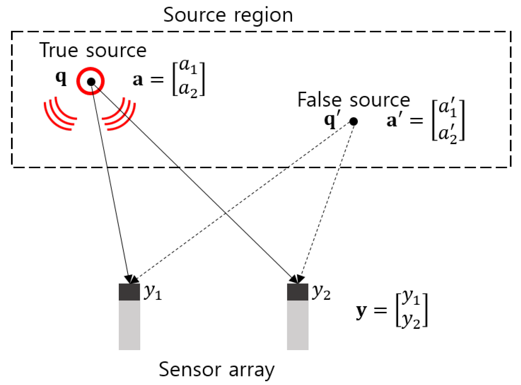
8) can be explained by the following example. Assume that a single monopole source is placed at
in a two-dimensional space, which is shown in
Figure 1. The sound pressure is measured by an array consisting of two sensors. A virtual source region is set with two points, one of which is the true source location. At frequency
f, the measured signals at the array are
and
. The propagation vectors can be calculated using Equation (
3), which are expressed as
and
.
For the true source point, Equation (
1) reduces to
Accordingly, the relation between the matrices
and
can be expressed as
Substituting Equation (
11) into Equation (
8) yields
As the left-hand side of Equation (
8) is a non-negative value, Equation (
12) shows that for the true source location, the cost function is minimized. For the false source location, this can be written as
It can be seen that the second term of the right-hand side of Equation (
13) depends on the propagation vector
, and thus, the cost function is always greater than zero.
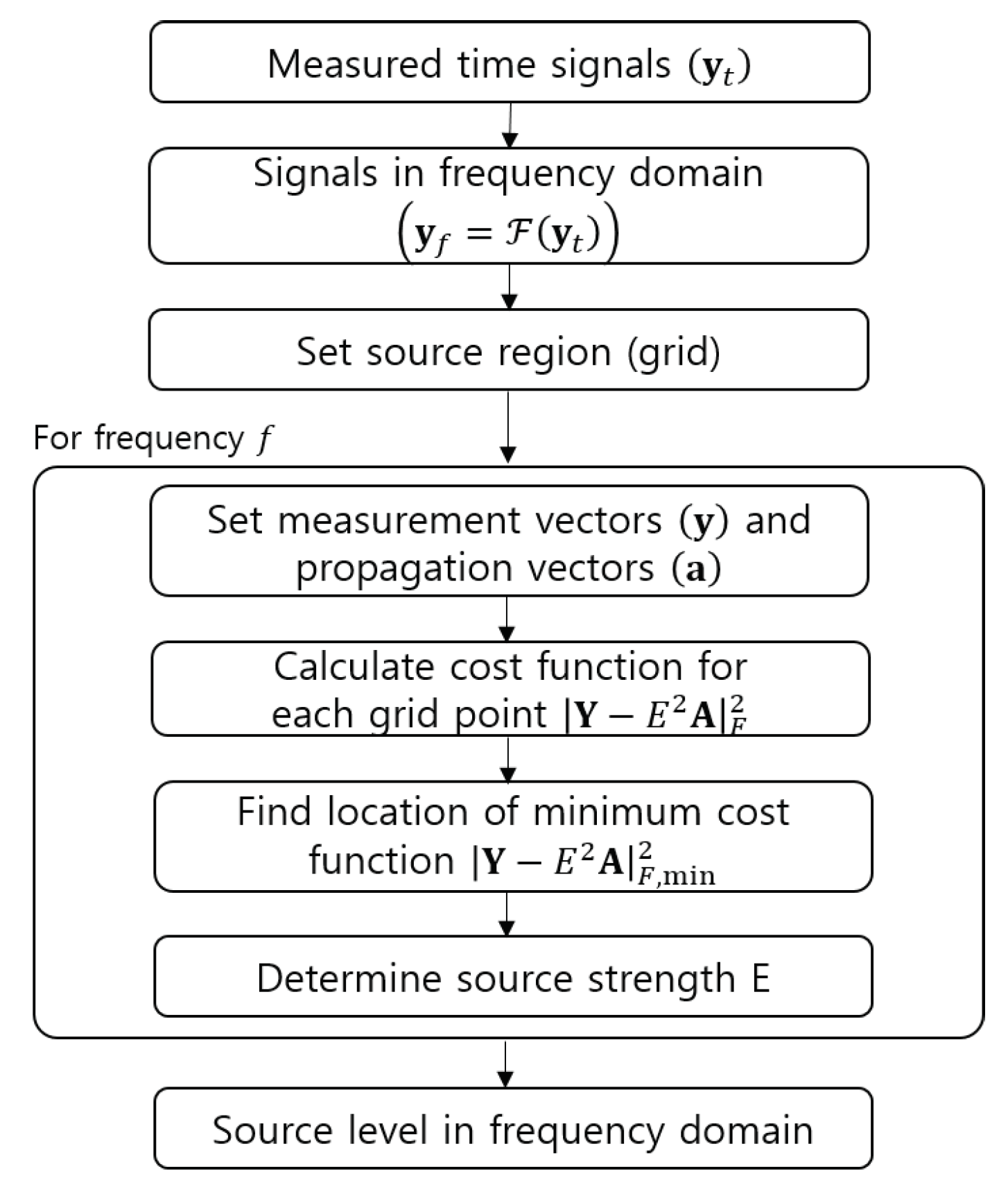
In the actual application, the cost function is calculated at each point in the source region and the point where the cost function is minimum is determined. The corresponding source strength
E is then calculated from Equation (
7). The whole procedure is summarized in
Figure 2. It should be noted that the method works well when the actual cavitation noise sources are concentrated within a single region because a single monopole source at a single point is assumed at each frequency.
2.2. Validation of the Method
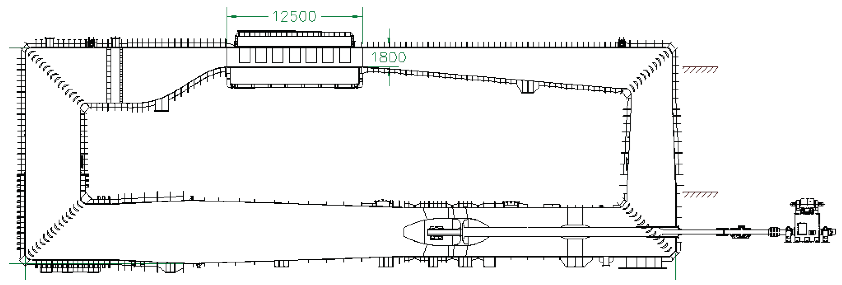
To check the validity of the estimation method, a model-scale measurement was conducted in the Large Cavitation Tunnel (LCT) at the Korea Research Institute of Ships and Ocean Engineering (KRISO).
Figure 3 shows a schematic view of the tunnel. The overall dimensions of the tunnel are 60 × 22.5 × 6.5 m
, and those of the test section are 12.5 × 2.8 × 1.8 m
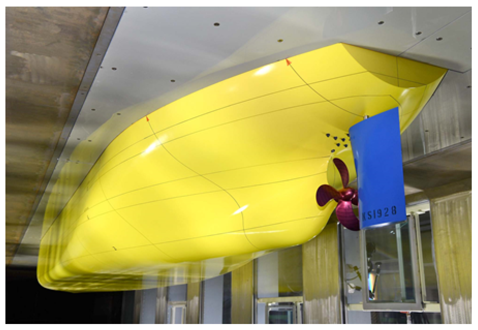
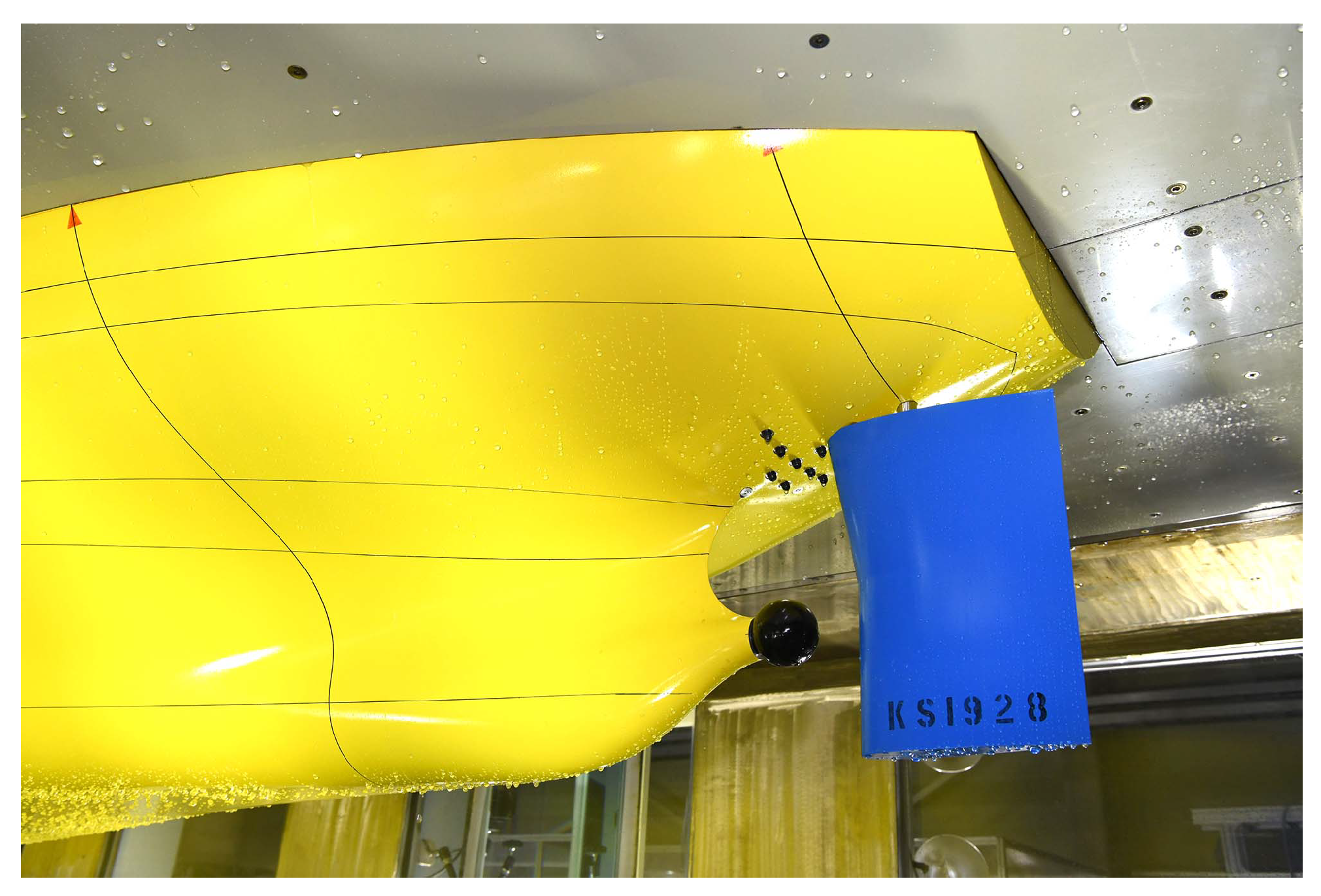
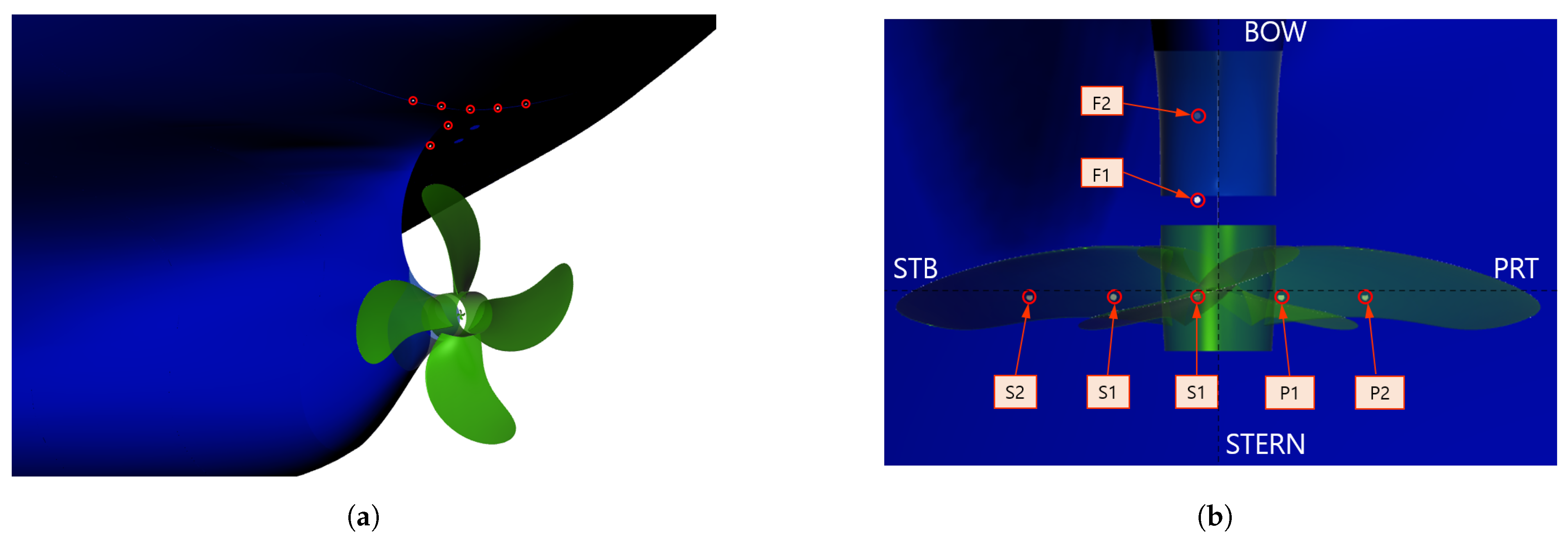
. A model ship and propeller with a scale ratio of 25.6 were installed in the test section, as shown in
Figure 4.
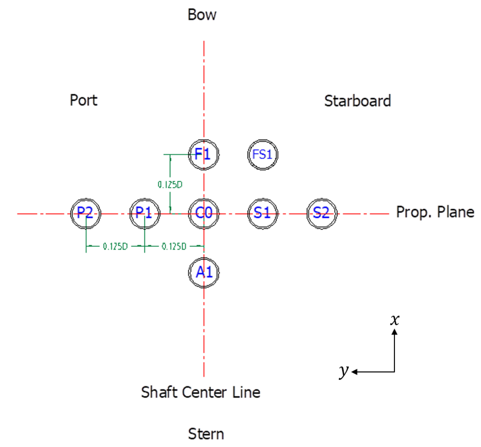
A set of B&K type 8103 miniature hydrophones were installed at the hull above the propeller plane for the estimation of source strength. The position and the coordinates of the hydrophones on the hull are shown in
Figure 5 and
Table 1, respectively. As the hydrophones were not flush-mounted, they were expected to be affected by flow noise. This would be small, however, unless cavitation were to occur directly around the hydrophones. All the hydrophone sensors were connected to a B&K type 2692-A charge amplifier and B&K type 3052 data acquisition system, which provided a sampling frequency of up to 204.8 kHz.
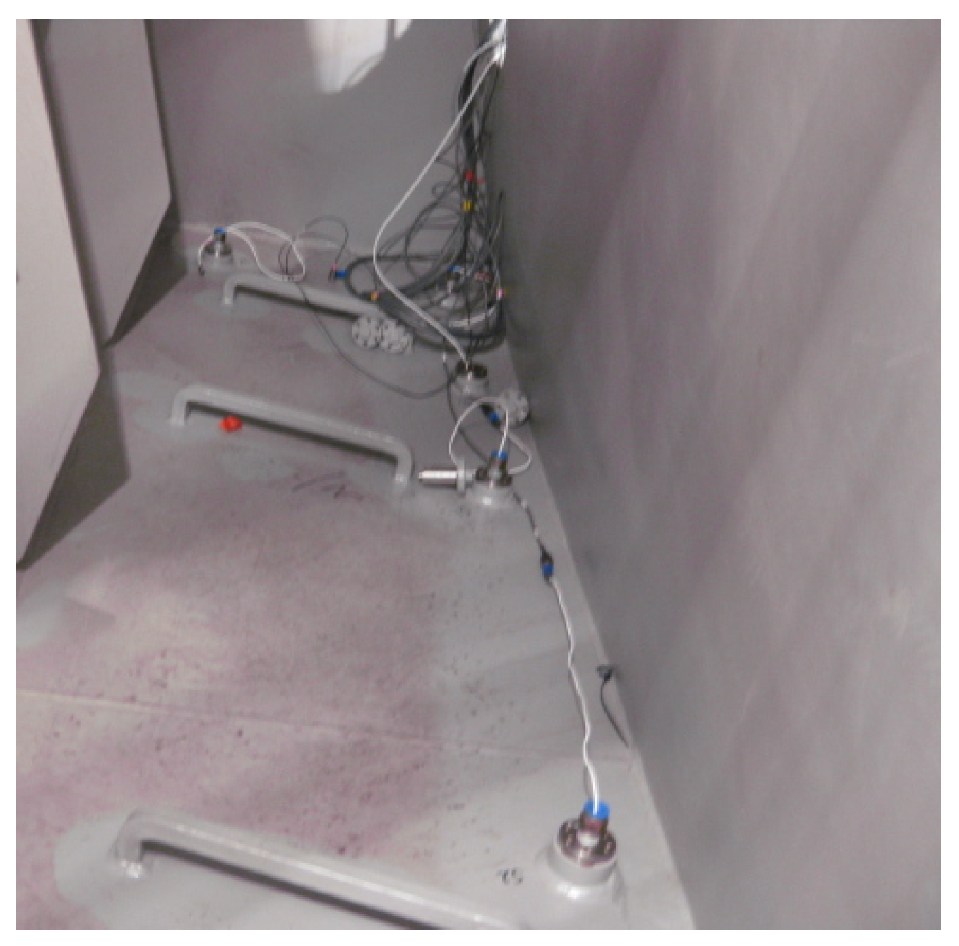
To obtain the source level from the measurement, a B&K type 8105 hydrophone was used in an acoustic window at the bottom of the tunnel. The test procedure was as follows. Firstly, the background noise was measured without the propeller in the presence of the flow. Secondly, the propeller noise was measured at the test condition. The background noise correction was then applied to obtain valid data (
). To calculate the source level, it was necessary to measure the transfer function between the source and the receiver. This could be done by replacing the propeller with a sound source of known properties and measuring the source and receiver signals simultaneously. Note that in the transfer function measurement, the flow speed was set to be zero. In this study, an ITC-1032 transducer was used, for which the setup is shown in
Figure 6. The transfer function measurement is usually carried out for different source positions along the propeller disk in the circumferential direction. However, only the center position was considered in this study, as the difference was negligible. To obtain more accurate results, one may look at the cavitation pattern to identify possible source locations.
The source level in model-scale measurements can be obtained as follows:
where
is the source level at the model scale,
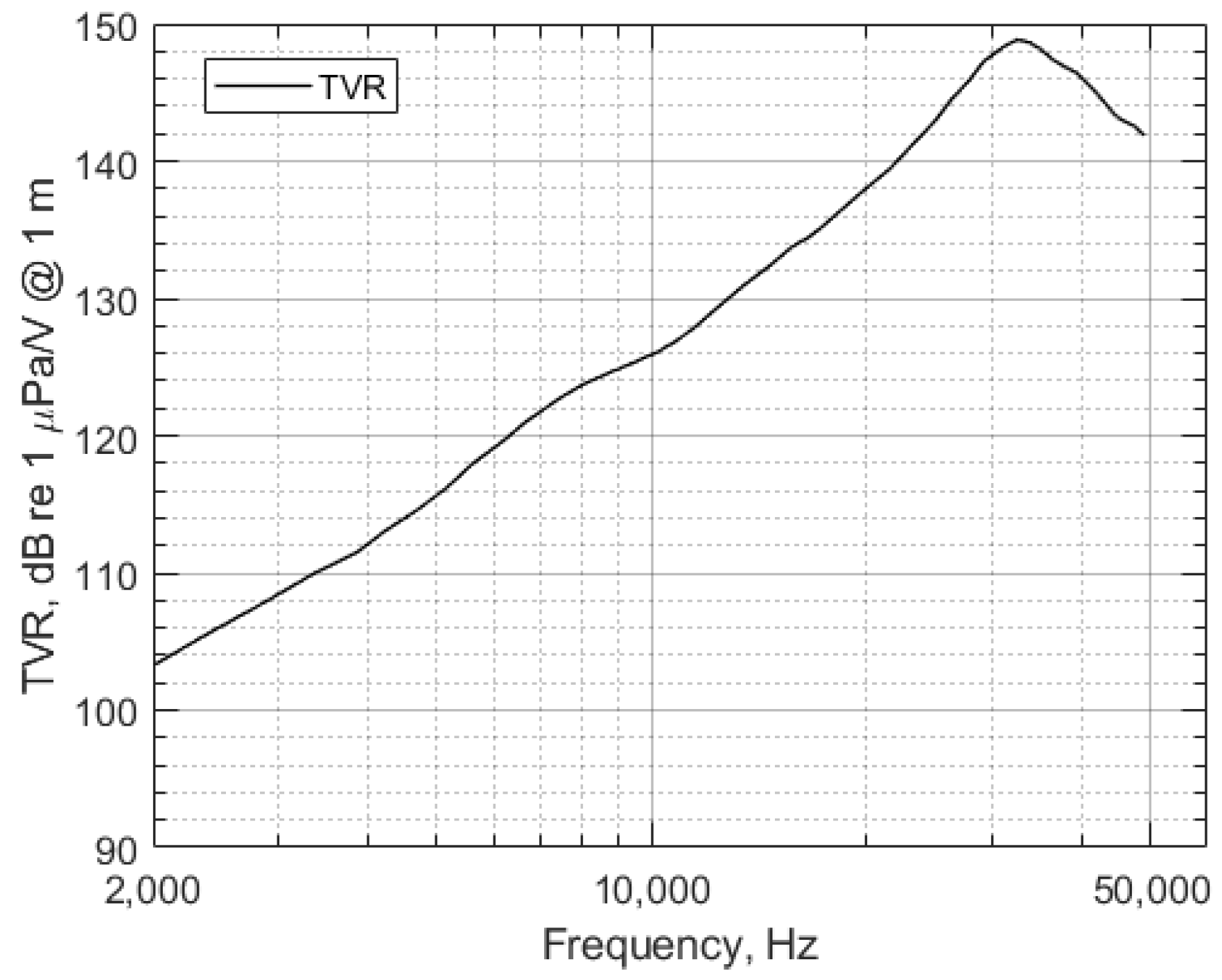
is the transmitting voltage response of the transducer in free field, and
is the transfer function. The transmitting voltage response was provided in the transducer data sheet, as shown in
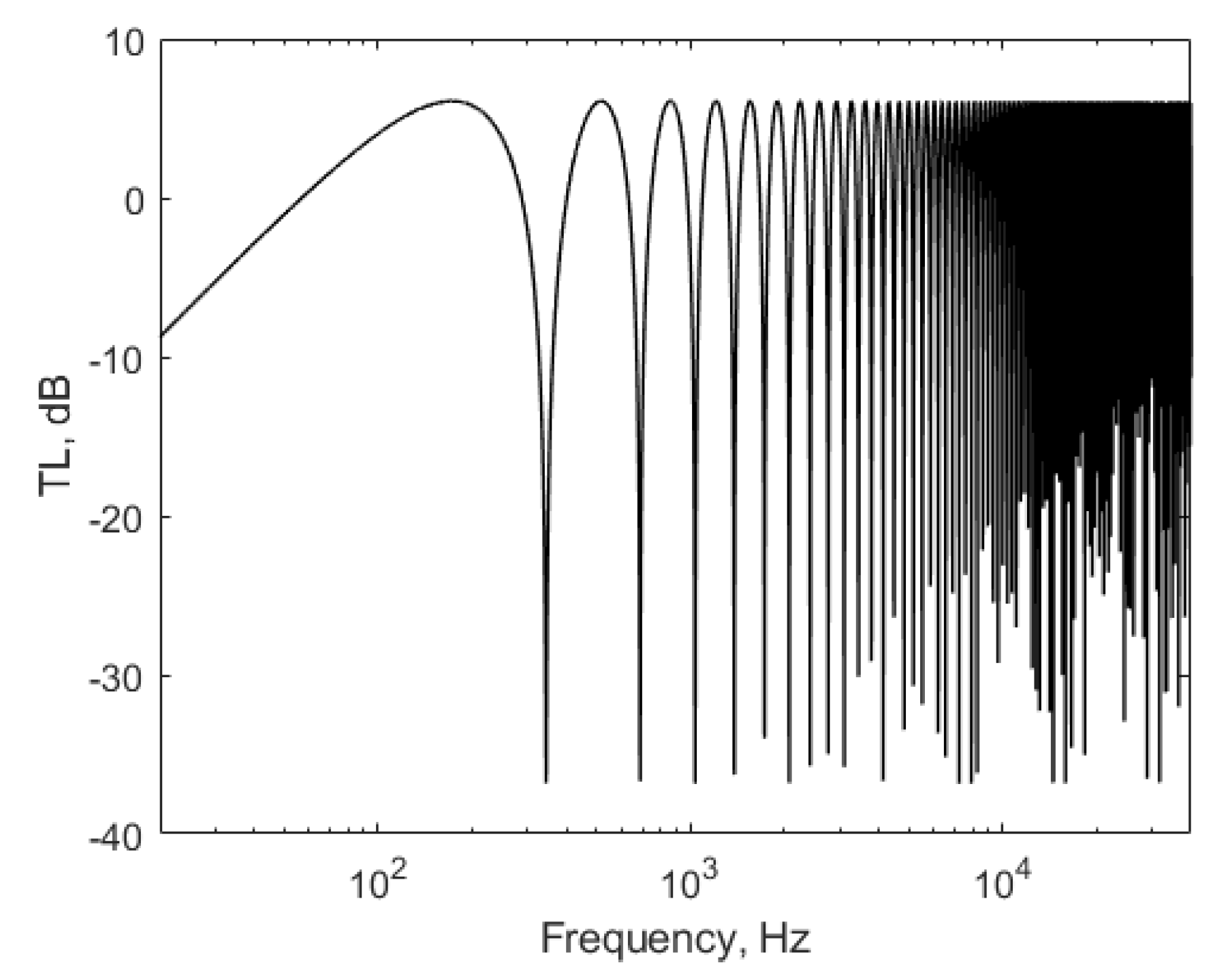
Figure 7. The transfer function between the source and the hydrophone in the tunnel was measured, and the result is shown in
Figure 8. Using these two graphs, the source level in free field can be obtained for a given operating condition.
Three operating conditions were considered in the measurement, as shown in
Table 2. Here, the cavitation number
is defined as
where
is the pressure at the center of the tunnel,
is the density of the fluid,
g is the gravitational acceleration,
is the height that is defined from the center of the tunnel to the
upward position,
is the vapor pressure,
n is the rotational speed of the propeller, and
D is the diameter of the propeller. The flow speed
V was set to be 7 m/s, and the tunnel pressure was controlled to tune the cavitation number. The water temperature was 16.3
C. Each run was recorded for 60 s with a sampling frequency of 204.8 kHz. The data were post-processed using MATLAB to obtain the power spectral density (PSD).
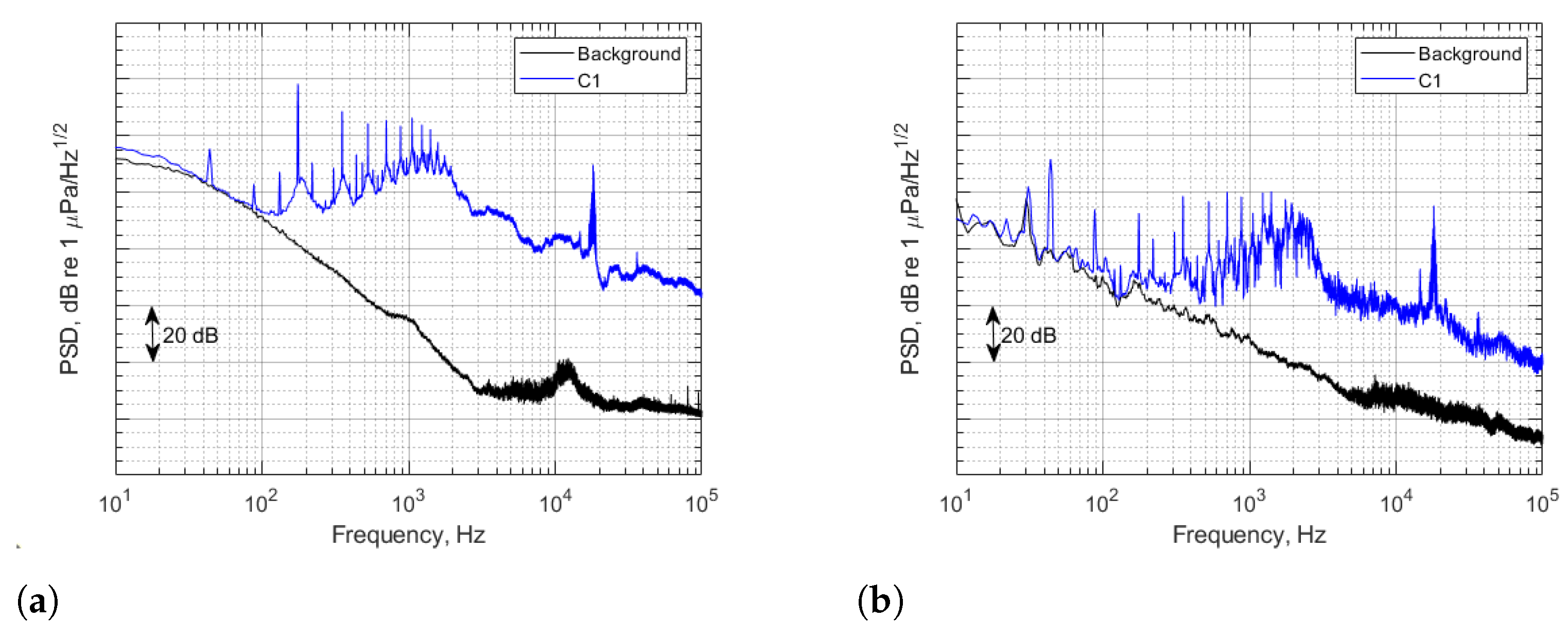
Figure 9 shows a comparison between the measured signals in operating condition
and the background noise. For the hull pressure sensors, the result at the “C0” position were plotted. From the graphs, it can be seen that the result above 200 Hz can be used without correction. However, the TVR of ITC-1032 is uncalibrated at frequencies below 2 kHz. Therefore, the result at frequencies above 2 kHz is valid. It is also seen that the shaft rate components and the blade rate components have a strong effect on the spectrum below 2 kHz. These components may not be estimated well, even if the transducer covers this frequency range, as monopole-like sound propagation is assumed. The cavitation noise is dominant above 2 kHz, where a smooth curve is seen. The peaks around 20 kHz are the singing noise caused by structural resonances at the trailing edge of the propeller blades.
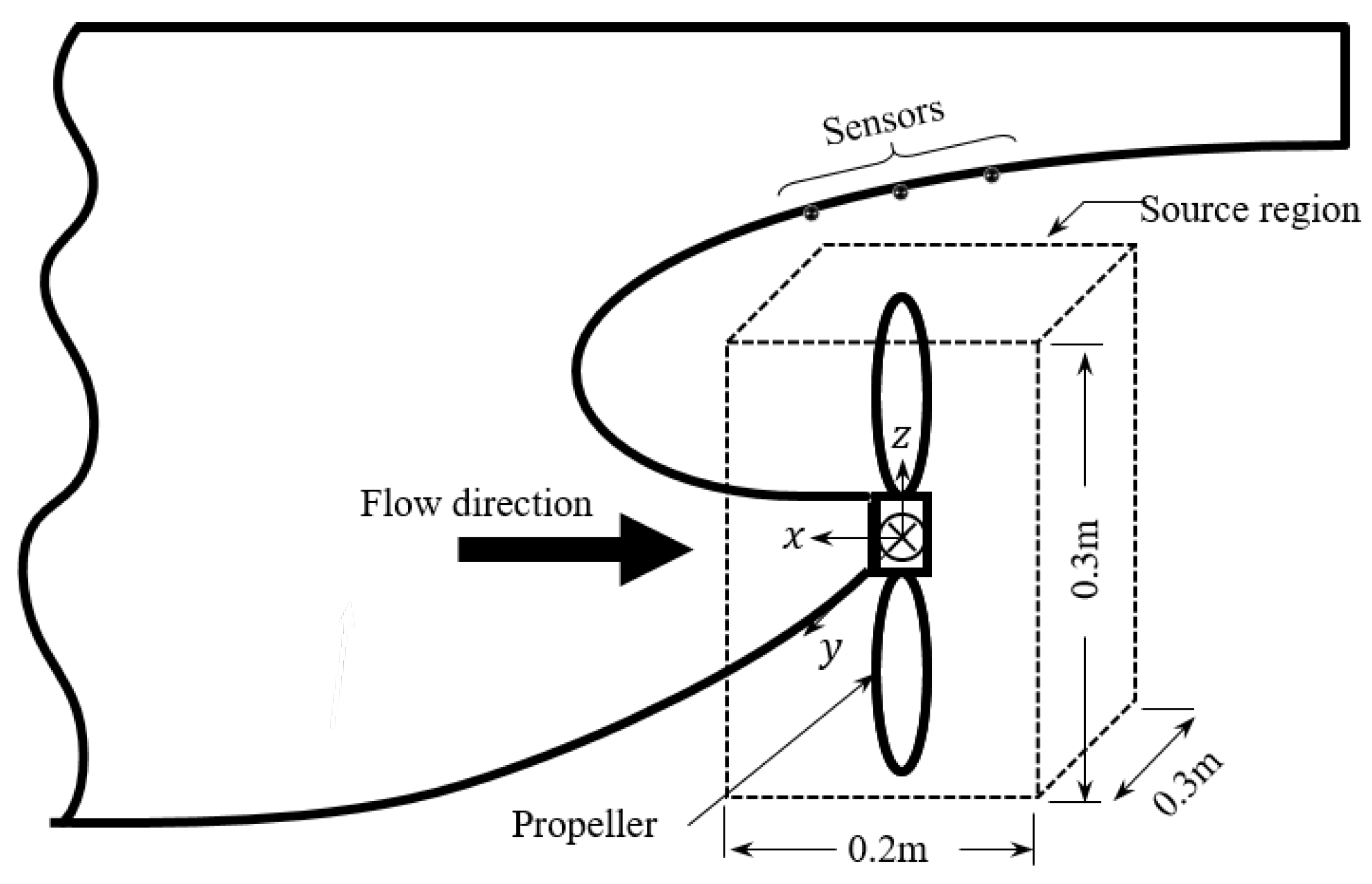
To calculate the source level, a hexahedral source region was set around the propeller, which is shown in
Figure 10. The ranges of
y and
z are defined symmetrically with respect to the propeller center, from −0.6
D to 0.6
D, where
D is the propeller diameter. The range of
x is defined from −0.1 to 0.1 m. The spacing was set to be 0.01 m in all directions.
The sound pressure measured from the sensors at the hull was converted using the Fourier transform. For the source-level estimation, the frequency range was set from 1 to 100 kHz with a spacing of 32 Hz. For the grid points in the source region,
was calculated.
Figure 11 shows the normalized values of
in the source region at 8 and 40 kHz, for example. A strong noise source is seen between the 12 o’clock position and 1 o’clock position viewed from the stern side. In addition, it can be seen that the source was located downstream close to the propeller. At 8 kHz, the source was located in one region, whereas two main source regions are seen at 40 kHz. For this reason,
is lower in the 40 kHz result.
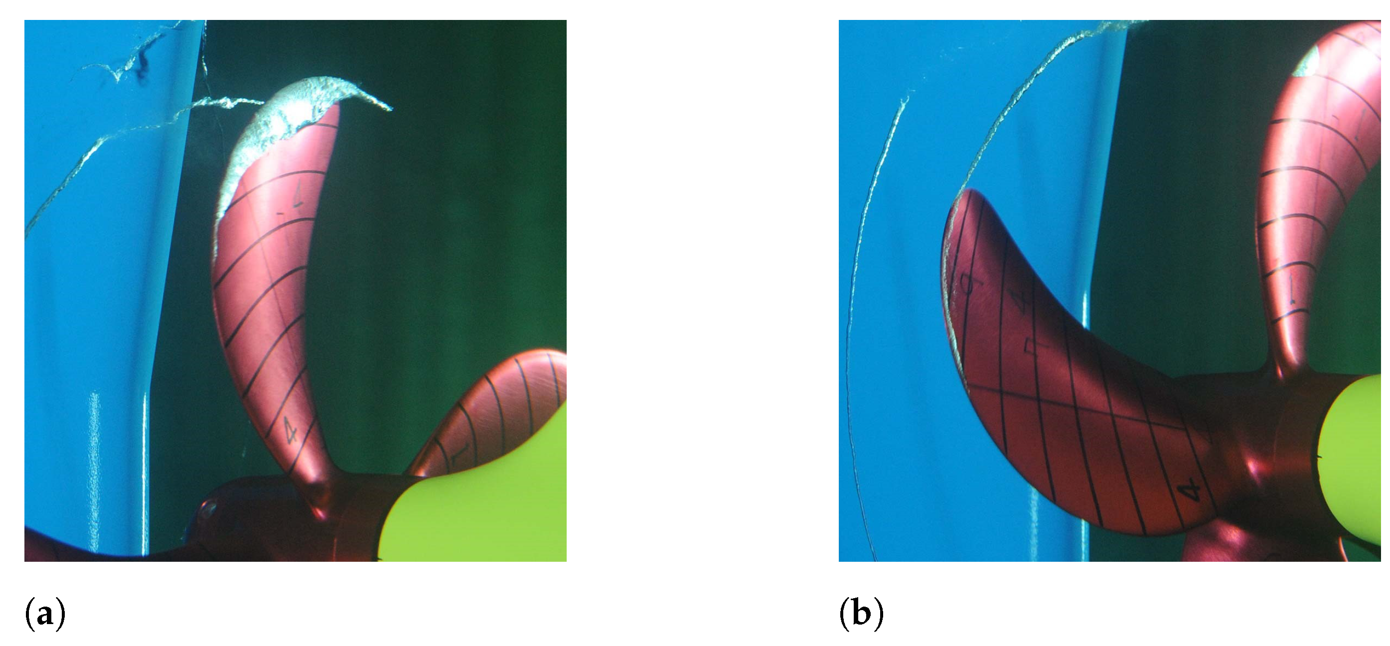
For comparison, the cavitation pattern for condition
is shown in
Figure 12. Note that the angle is defined at the 12 o’clock position viewed from the stern side in the clockwise direction. It can be seen that the cavitation occurs strongly on the starboard side, which is also found in
Figure 11. Thus, it can be said that the method reasonably describes the noise source.
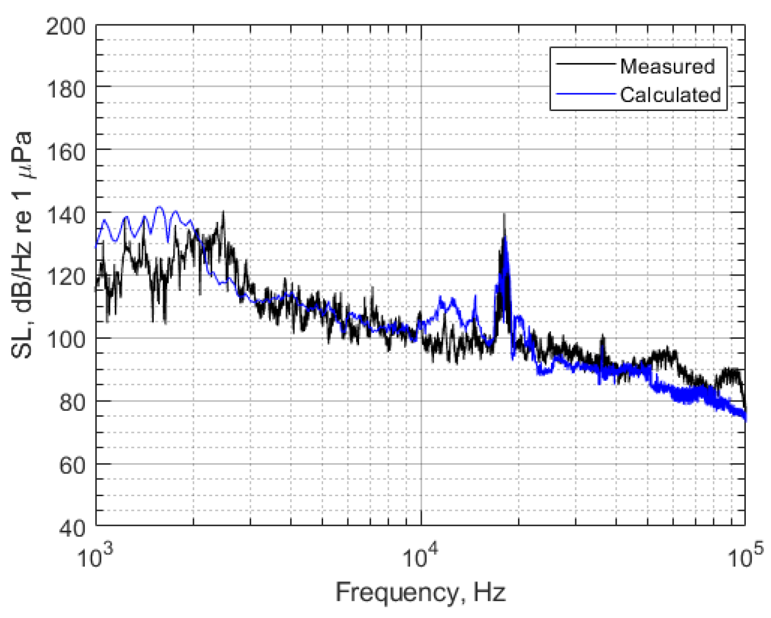
From the
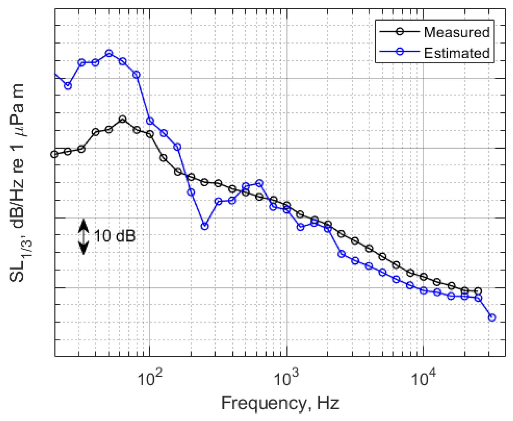
map, the maximum value was found, and the corresponding source level was obtained. Having obtained the source level at all frequencies, the result was compared with the measured source level, which is shown in
Figure 13 in terms of spectral density. Overall, the calculated source level agreed well with the measured one from 2 to 50 kHz. The differences below 2 kHz were due to the combination of the monopole assumption and the transducer characteristics. Above 50 kHz, the transfer function could not be applied, and thus, the predicted source level deviated from the measured one. From this, it can be said that the proposed method is valid.
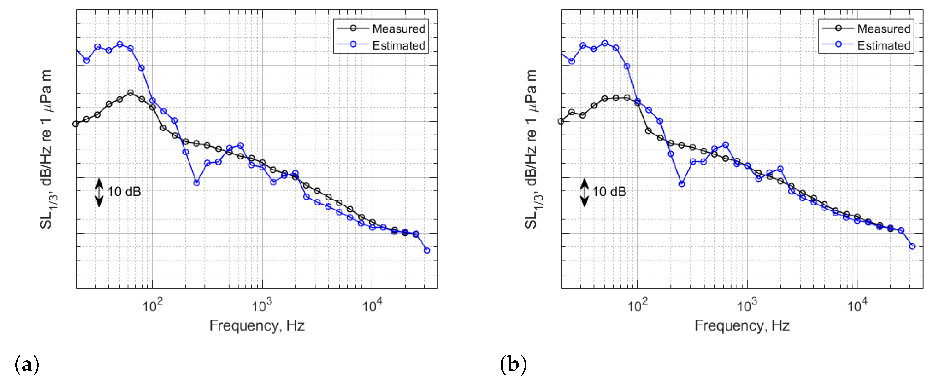
Comparisons were also made for the other conditions. This is illustrated in
Figure 14. The same conclusion can be drawn, with few differences in the results.


