Low-Cost Calibration of Matching Error between Lidar and Motor for a Rotating 2D Lidar

Abstract

For a rotating 2D lidar, the inaccurate matching between the 2D lidar and the motor is an important error resource of the 3D point cloud, where the error is shown both in shape and attitude. Existing methods need to measure the angle position of the motor shaft in real time to synchronize the 2D lidar data and the motor shaft angle. However, the sensor used for measurement is usually expensive, which can increase the cost. Therefore, we propose a low-cost method to calibrate the matching error between the 2D lidar and the motor, without using an angular sensor. First, the sequence between the motor and the 2D lidar is optimized to eliminate the shape error of the 3D point cloud. Next, we eliminate the attitude error with uncertainty of the 3D point cloud by installing a triangular plate on the prototype. Finally, the Levenberg–Marquardt method is used to calibrate the installation error of the triangular plate. Experiments verified that the accuracy of our method can meet the requirements of the 3D mapping of indoor autonomous mobile robots. While we use a 2D lidar Hokuyo UST-10LX with an accuracy of ±40 mm in our prototype, we can limit the mapping error within ±50 mm when the distance is no more than 2.2996 m for a 1 s scan (mode 1), and we can limit the mapping error within ±50 mm at the measuring range 10 m for a 16 s scan (mode 7). Our method can reduce the cost while the accuracy is ensured, which can make a rotating 2D lidar cheaper.

1. Introduction

As an environmental modeling sensor, lidar is widely used. Typically, lidar can be divided into 2D lidar and 3D lidar, 3D lidar can scan 3D surfaces and obtain 3D maps of surroundings, but it is usually quite expensive. While the price of 2D lidar is relatively cheap, it can only obtain 2D maps which contain less information than 3D maps. However, if a 2D lidar is moved in a certain direction, it can be used to scan a 3D surface [1]. By moving a 2D lidar, one can model a 3D environment at low cost. Thus, a moving 2D lidar can replace (or at least partially replace) a commercial 3D lidar in many applications, avoiding the expensive cost of using a 3D lidar.

To build a moving 2D lidar, a common way is to install a 2D lidar on a motor shaft, so that a rotating 2D lidar is built [2,3]. The data collected by a 2D lidar is combined with the rotation angle of a motor, and the 3D coordinates of the points are calculated. Research on rotating 2D lidars can be divided into two categories, one is how to eliminate the error of the 3D point cloud while a rotating 2D lidar is working in a static environment [1,2,3,4,5,6,7,8,9,10,11,12,13,14,15,16,17,18,19,20,21,22,23], the other is how to correct the distortion of the 3D point cloud while a rotating 2D lidar is working in dynamic environment [24,25,26,27,28]. In this paper, we focus on the former question, that is, how to eliminate the error of a rotating 2D lidar while it is working in a static environment.

This question can be further divided into two subcategories. One is to calibrate the mechanical error between the lidar and the rotating unit [1,4,5,6,7,8,9,10,11,12,13,14,15]. Due to the mechanical error, the relative position and attitude between the 2D lidar and rotating unit are not exactly the same as expected. The error is 6-degrees of freedom (DOF), containing a 3-DOF translation and 3-DOF rotation [4]. The mechanical error can decrease the accuracy of the 3D point cloud in many aspects, including the shape and attitude of the 3D point cloud. The mechanical error is inevitable because machining and assembling errors cannot be eliminated completely. Therefore, calibration is necessary.

The other subcategory is to calibrate the matching error between the 2D lidar and rotating unit (that is, the motor) [2,3,5,8,16,17,18,19,20,21,22,23]. The working principle of a rotating 2D lidar is to calculate the 3D coordinates of the points by using the data collected by the 2D lidar and the angle of the motor shaft. Therefore, in order to improve the accuracy of the 3D point cloud, it is necessary to match the data from the 2D lidar and the angle of the motor shaft accurately. If we can know the angle of the motor shaft corresponding to each point collected by the 2D lidar during the entire 3D scan of a rotating 2D lidar, the matching error between the 2D lidar and the motor can be eliminated. However, in reality, the situation mentioned above does not exist, so the matching error always exists, which has a negative impact on the accuracy of the 3D point cloud, both in shape and attitude.

The first subcategory focuses on the calibration of the mechanical error, and the second subcategory focuses on the calibration of the matching error. They are juxtaposed with each other and cannot be replaced by each other. Only when both the mechanical error and the matching error are calibrated, a rotating 2D lidar can get an accurate 3D point cloud in a static environment.

The first subcategory, the calibration method of the installation error between the 2D lidar and the rotating unit, has been thoroughly evaluated. For example, the calibration processes proposed in [1,4,5] can work effectively without the need of specific scene, additional equipment, and a priori information about the environment (such as size etc.). The requirement is that there should be at least one plane in the scanning field. Planar features are abundant in man-made indoor environments, such as walls, floors, and ceilings.

However, the research on the second subcategory is relatively unexplored. The existing methods used for calibration of the matching error between a 2D lidar and motor mostly utilize expensive servo motors or encoders to output the motor rotation angle with the time stamps, and align it with the data form 2D data with time stamps. In this way, the matching error is calibrated [2,3,5,8,16,17,18,19,20,21,22,23]. Although for installation error, which is mentioned in the first subcategory, the calibration can be done at zero cost, without the need of additional equipment and all the work can be accomplished in normal indoor environment, while the calibration of the matching error is still expensive, for a servo motor or encoder is needed. Therefore, it is worthwhile to figure out a way to calibrate the matching error at low cost.

For the calibration of the matching error, the commonly used method is to align the data from the 2D lidar and the angle of the motor shaft by time stamps. Since the frequency of the two types of data is different, interpolation is used to obtain matched data pairs. The prerequisite for using this method is that the rotating unit that rotates the 2D lidar can output the absolute angle position of its shaft, which requires expensive device such as a servo motor or encode. This method has been used in [3,5,16,17,18,19]. A similar method was used in [2,8,20], for each time, when a group of data from the 2D lidar is received, the angle of the motor shaft at this moment is recorded. According to the serial number of each data in this group, its corresponding motor shaft angle can be estimated linearly. In [21], a pitching 2D lidar was built. In this work, a high-precision potentiometer was used to measure the angle of the motor shaft. In [22], a rotating 2D lidar used on an unmanned aerial vehicle (UAV) was built, and the software package Spin_Hokuyo [23] was used to generate the 3D point clouds in real time. The applicable hardware for Spin_Hokuyo is a 2D lidar UTM-30LX Hokuyo and a servo motor Dynamixel MX-28, while the servo motor Dynamixel MX-28 also can output the rotation angle. In order to facilitate the use of this software package, the above hardware was used in [22]. In addition to the above literature, the rotating units in [9,29] were stepper motors, without using encoders. The matching error was neglected, the matching between the 2D lidar and the motor was done through rough estimation, merely.

According to [2,3,5,8,16,17,18,19,20,21,22,23], in order to accurately match the 2D lidar and the motor, the rotating unit must be able to output the absolute angle position of the motor shaft. Therefore, a device like a servo motor or encoder is necessary. This goes against the idea of reducing costs. The reason why we built a rotating 2D lidar instead of using a commercial 3D lidar directly is because we wanted to reduce costs. The high price of commercial 3D lidars makes them unaffordable for many users, and the cost of a rotating 2D lidar is one-tenth of it. The obvious advantage of a rotating 2D lidar over a commercialized 3D lidar is the lower cost. Therefore, for a rotating 2D lidar, the question of how to further reduce its cost under the premise of ensuring accuracy is worth studying.

If a rotating 2D lidar is not equipped with an encoder or a servo motor, and only a stepper motor is used as the rotating unit, the cost can be further reduced. However, the angle of the motor shaft cannot be measured, because of which, the 2D lidar and the motor cannot be accurately matched according to the existing methods. This will reduce the accuracy of the 3D point cloud.

In this paper, we focus on the low-cost calibration of matching error between the lidar and the motor for a rotating 2D lidar. Compared with the existing methods, our method reduces the cost. In order to reduce the cost, we did not use a sensor to measure the angle of the motor shaft in our prototype, because it is expensive. We calibrated the matching error between the 2D lidar and the motor without using a servo motor or encoder. A stepper motor was used to rotate the 2D lidar, photoelectric switch and shading sheet were used to define the initial position of the motor shaft, a triangular plate was used to calibrate the matching error between the 2D lidar and the motor. While reducing the cost of a rotating 3D lidar, our method ensured the accuracy of the 3D point cloud. Our method provides a new idea for the further cost reduction of a rotating 2D lidar.

The rest of this paper is structured as follows. Section 2 describes the problem to be solved in this paper; the modeling of the system is described in Section 3. The calibration method is described in detail in Section 4. Then, we verify our method by experiments in Section 5. Finally, a brief conclusion and future work are given in Section 6.

The notations used throughout this paper have been listed in

Table A1. Nomenclature.

Symbol	Explanation
γ	Angular resolution of rotating 2D lidar in the direction of motor shaft.
n	Number of 2D lidar scans included in a 3D scan.
f	The scanning frequency of 2D lidar is f, which can be found in its product manual.
T	The time used by a 3D scanning of a rotating 2D lidar is T.
ω	The Angular velocity of the motor shaft in a rotating 2D lidar is ω.
L	The coordinate frame of 2D lidar.
O’	The coordinate frame of rotating unit (before attitude correction).
O	The coordinate frame of rotating unit (after attitude correction).
r	Ranging data of 2D lidar.
θ	The azimuth angle in the scanning sector of the 2D lidar corresponding to the ranging data r.
pL	A 3D point with respect to coordinate frame L, it is calculated according to the data of 2D LIDAR.
${\mathit{R}}_L^{O^{\prime }}$	Rotation matrix from coordinate frame L to coordinate frame O’ at the moment when a 3D scan of a rotating 2D lidar is started.
${\mathit{t}}_L^{O^{\prime }}$	The translation vector from coordinate frame L to coordinate frame O’ at the moment when a 3D scan of a rotating 2D lidar is started.
φmotor	Rotation angle of the motor shaft corresponding to the ranging data r.
RM	The rotation matrix calculated according to the rotation angle φmotor of the motor shaft.
K	The total number of points in the 3D point cloud obtained by a 3D scan of a rotating 2D lidar.
k	The ordinal number of a point in all points of a 3D point cloud.
pO’	A 3D point with respect to coordinate frame O’, which is converted from point pL in coordinate frame L.
φoffset	The deflection angle of the coordinate frame O’ relative to the coordinate frame O in the Z-axis direction.
${\mathit{R}}_{O^{\prime }}^O$	The rotation matrix calculated according to φoffset.
pO	A 3D point with respect to coordinate frame O, which is converted from point pO’ in coordinate frame O’.
CO’	A 3D point cloud with respect to coordinate frame O’, which is collected by a rotating 2D lidar.
Ctri	A point cloud corresponding to the triangular plate extracted from the point cloud CO’.
c	The center point of the triangular plate.
α	The angle between the middle line of the triangular plate and the front direction of the prototype (which is also the positive direction of the axis X of coordinate frame O).
β	The angle between the middle line of the triangular plate and the axis X’ of the coordinate frame O’.
CO	A 3D point cloud with respect to coordinate frame O, which is converted from point cloud CO’ through rigid body transformation.
n1~n4	The unit normal vectors of the planes corresponding to the 4 walls of the room in the point cloud CO, respectively.
i, j	The unit normal vectors corresponding to X-axis and Y-axis of coordinate frame O, respectively.
Eatti	The attitude error of point cloud CO, which is expressed as the sum of absolute values of vector inner product.
φerror	The attitude error of point cloud CO, which is expressed as an angle.
${\mathit{R}}_{\mathrm{error}}$	The rotation matrix calculated according to the angle φerror.
$f\left({\phi }_{\mathrm{error}}\right)$	A function showing the attitude error of the point cloud CO, with φerror as the independent variable.
fcost(α)	A function showing the attitude error of the point cloud CO, with α as the independent variable.
M	The total number of 3D scans used for the calibration of the installation error of the triangular plate.
m	The serial number of a 3D scan while calibrating the installation error of the triangular plate.
$F_{\mathrm{cost}}(\alpha )$	The total attitude error of point cloud CO, which is expressed by least square method.
N1~N4	Data sets, formed by n1~n4 from 50 point clouds CO, respectively.
kitera	Parameter of Algorithm A1, the serial number of a iteration.
kmax	Parameter of Algorithm A1, the maximum times of iteration.
α0	Parameter of Algorithm A1, the initial value of α.
ε1	Parameter of Algorithm A1, the first stopping criteria of the algorithm.
ε2	Parameter of Algorithm A1, the second stopping criteria of the algorithm.
J(α)	Parameter of Algorithm A1, Jacobian matrix.
A	Parameter of Algorithm A1, A = J(α)TJ(α).
g	Parameter of Algorithm A1, g = J(α)T Fcost(α).
μ	Parameter of Algorithm A1, the damping parameter.
τ	Parameter of Algorithm A1, a coefficient which is used to determine the initial value of μ.
v	Parameter of Algorithm A1, a coefficient which is used to adjust the value of μ in each iteration.
aii	Parameter of Algorithm A1, the element in A.
I	Parameter of Algorithm A1, unit matrix.
Δα	Parameter of Algorithm A1, the gain of α in each iteration.
ρ	Parameter of Algorithm A1, gain ratio.
d	The distance from the object to a rotating 2D lidar.
Emap	The error of the 3D map at distance d, the map is obtained by a rotating 2D lidar which is calibrated by our method.

, which is in Appendix A.

2. Problems

According to the previous description, our goal is to use only a stepper motor to rotate a 2D lidar without using encoder or servo motor to reduce the cost under the premise of ensuring the accuracy of the 3D point cloud. For this purpose, a method is proposed in [2], an open-loop controlled stepper motor is used to rotate the 2D lidar, the motor stops rotating when its shaft turns to a certain position, and then the 2D lidar begin its scan. After the 2D lidar finishes scanning, the motor shaft rotates to the next position, and the 2D lidar scans again. This cycle continues until the 3D point cloud collection is completed. There is a certain angle between every two adjacent positions of the motor shaft, which determines the density of the 3D point cloud. This method attempts to align the data from the 2D lidar and the angle of the motor shaft at the cost of low efficiency, but it has obvious disadvantages. The frequent stop and start of the motor may cause mechanical failure. The acceleration and deceleration of the motor can decrease the accuracy of the rotation positioning. Due to the need of stopping the rotation of the motor shaft for multiple times, the time used for finishing a 3D scan will be prolonged. In view of the above disadvantages, it is necessary to develop a method to calibrate the matching error between 2D lidar and motor while the motor rotates continuously.

In our work, during the 3D scan process of a rotating 2D lidar, the 2D lidar scans continuously, and the shaft of the stepper motor rotates at a constant angular velocity. The matching between the two can no longer be done with the help of time stamps, because the stepper motor is open-loop, and there is no sensor to measure the rotation angle of the motor shaft, so the data of motor angle with time stamps cannot be obtained.

In this case, we initially tried to match the 2D lidar and the motor in the following way. After the angular resolution γ in the direction of motor shaft rotation was configured, the number of scanning cycles n of the 2D lidar in one 3D scan could be calculated as:

$$n=\frac{180°}{\gamma }$$

(1)

The scanning frequency f of the 2D lidar could be found in its product manual, so the time T used for finishing a 3D scan of a rotating 2D lidar could be calculated as:

$$T=\frac{n}{f}$$

(2)

For a rotating 2D lidar, a 3D scan requires the motor shaft to rotate 180 degrees [2], so the angular velocity ω of the motor shaft could be calculated as:

$$\omega =\frac{180°}{T}$$

(3)

Until now, the control parameters of the 2D lidar and the stepper motor have been calculated, the working time of the 2D lidar in continuous scanning mode is T, the shaft of the stepper motor rotates at angular velocity ω, and its working time is T. We made them start working at the same time, so that ideally they could be matched.

However, we found that there are obvious errors in the 3D point cloud, both in the shape and attitude. Additionally, for each 3D scan, the error is not constant. Our experiment is shown in Figure 1, Figure 1a is a photo of the environment for collecting 3D point cloud. The errors we observed are shown in Figure 1b,c. The environment is a conference room. The position of the rotating 2D lidar is aligned with the gap between the tiles on the ground to ensure that it is not skewed relative to the conference room. In this way, the top view of the 3D point cloud should be correct in shape and attitude, and coincide with the blue wireframe. This is not actually the case. The shape is distorted and the attitude is skewed. In addition, for each 3D scan, the error of the 3D point cloud is uncertain, and the 3D point cloud may appear as in Figure 1b,c.

There are several reasons for the error.

(1)

As mentioned in [1,4,5,6,7,8,9,10], the mechanical error between the 2D lidar and rotating unit can cause distortion of the 3D point cloud. Based on the idea of control variables, in order to focus on other reasons, we need to exclude this item first. By improving the manufacture and assembly accuracy of the mechanical parts of our prototype, we minimized the impact of mechanical errors on the accuracy of the 3D point cloud. We used computer numerical control (CNC) machine tools to manufacture the key parts of our prototype, with a tolerance level of IT5 (Chinese standard, GB/T1184-1996). In Appendix B, we verified that the self-reasons of our prototype (which include the mechanical error) has a much smaller impact on the accuracy of the 3D point clouds than the error of the 2D lidar itself (±40 mm). Therefore, we can exclude this item and assume that other reasons are causing the resulting observed error.

(2)

The acceleration and deceleration of the motor shaft will cause error. In a 3D scan of a rotating 2D lidar, we assume roughly that the shaft of the stepper motor rotates at angular velocity ω for time T, and it rotates 180° in total. However, in practice, the motion of the motor shaft is more complex. The motor shaft accelerates from standstill to angular velocity ω, and then it keeps rotating at this speed, after which it decelerates to standstill. We have ignored the acceleration and deceleration of the motor shaft, and this can lead to the shape error of the 3D point cloud, which is especially obvious at the closed position of the point cloud. The so-called closed position here refers to the area where the points collected by the 2D lidar when the motor shaft starts to rotate or stops rotating. The areas of these two types of points are adjacent, and these points are most directly affected by the acceleration and deceleration of the motor shaft.

(3)

The use of photoelectric switches may cause error. Since no encoder or servo motor is used, it is necessary to define the initial position of motor shaft by photoelectric switch. When finding the initial position, the motor shaft will rotate back and forth by a large margin and make the shading sheet which rotates with the motor shaft triggering the photoelectric switch. After the photoelectric switch is triggered, the controller sends a stop command to the motor to stop its shaft. The position of the motor shaft after it stops is considered to be the initial position. This process can be described in more detail, the shading sheet blocks the light beam of the photoelectric switch—the photoelectric switch is triggered—the controller sends the stop command to the stepper motor—the shaft of stepper motor decelerates until it stops. The accuracy of the initial position of the motor shaft is affected by many factors such as the response time of the photoelectric switch, the rotation direction and the speed of the motor shaft. For each 3D scan of a rotating 2D lidar, the motor shaft starts rotating from its initial position. Therefore, if the initial position of the motor shaft is not accurately defined, the attitude error of the 3D point cloud will be caused.

(4)

The uncertain time deviation may cause error. In the actual engineering operation, we found that although we require the 2D lidar and the stepper motor to start to work at the same time, there is an uncertain time deviation between the starting time of the 2D lidar and the starting time of the stepper motor. The value of this time deviation is very small, but it is enough to have a significant impact on the accuracy of the 3D point cloud. The reason for the uncertain time deviation is that the response time of the 2D lidar and stepper motor to the command is inconsistent and not constant, as mentioned in [16]. Because both the transmission of the command and the response of the motor or the 2D lidar take time, there is an uncertain time deviation between the time when the controller starts to send the command to the motor and the time when the motor starts to work. Similarly, there is an uncertain time deviation between the time when the controller starts to send the command to the 2D lidar and the time when the 2D lidar starts to work. The uncertainty of the transmission time of the command and the response time of the device is a common problem which is difficult to solve. Because of this problem, we can mark the time when the controller starts to send the command to the motor or the 2D lidar in the program, we cannot know the actual working time of the motor or 2D lidar. This is the cause of the uncertain time deviation between the starting time of the 2D lidar and the starting time of stepper motor. For each 3D scan of a rotating 2D lidar, this time deviation is uncertain, so the shape and attitude error of the 3D point cloud for each scan is also uncertain (see Figure 1). The reason for the shape error of the 3D point cloud can be analyzed as follows. Due to the uncertain time deviation, there may be two situations. One is that the motor starts to rotate after the 2D lidar has started scanning continuously for a short period of time. The 3D point cloud collected in this case is shown in Figure 1b. At the position where the motor starts to rotate (the beginning of the yellow circular arrow), there is a shape error marked by red line. The other situation is that the motor starts working earlier than the 2D lidar, so that the motor has stopped rotating before the 2D lidar stops scanning. The 3D point cloud collected in this case is shown in Figure 1c. At the position where the motor stops rotating (the end of the yellow circular arrow), there is a shape error marked by red line. In either case, a shape error of the 3D point cloud will result. In addition, the attitude error can also be caused. Therefore, the uncertain time deviation between the starting time of the 2D lidar and the starting time of stepper motor is one of the reasons for the uncertain error of the 3D point cloud in shape and attitude.

In addition to item 1 of the above 4 items, it is our work to exclude the errors in the other three items. Unfortunately, these three errors mentioned above may be uncertain, for the acceleration and deceleration curve of the motor shaft may be uncertain, the response time of the photoelectric switch may be uncertain, especially, the time deviation between the moment when the 2D lidar starts to work and the moment when stepper motor starts to work may be uncertain, too. Due to the above uncertainties, the shape and attitude error of the 3D point clouds may also be uncertain.

The effect of item 2, 3 and 4 on the 3D point cloud can be divided into two categories, one is shape error and the other is attitude error, as shown in Figure 1. For simplicity, we first only analyze the shape error of the 3D point cloud.

According to Formulas (1)–(3), we can find that if the shape of the 3D point cloud is correct, the necessary and sufficient condition is that the stepper motor rotates at constant angular velocity ω during the continuous scanning of the 2D lidar. The acceleration and deceleration of motor shaft in item 2 will cause the shape error of the 3D point cloud. We have tried to estimate the approximate speed curve of the motor shaft, and to eliminate the shape error of the 3D point cloud. It turns out that this is not feasible. First, the acceleration and deceleration curve of the motor shaft may not be constant. Second, the shape error of the 3D point cloud is not entirely attributed to the acceleration and deceleration of motor shaft. The uncertain time deviation in item 4 also has a significant impact on the shape of the 3D point cloud. Therefore, the shape error of 3D point cloud cannot be effectively eliminated by estimating the approximate speed curve of the motor shaft.

If the action sequence of the 2D lidar and the stepper motor is modified, making the motor start to work earlier and stop working later than the 2D lidar, the acceleration and deceleration of motor shaft will be staggered with the working time of the 2D lidar, as shown in Figure 2. In this way, before the continuous scanning of the 2D lidar, the shaft of the stepper motor has been accelerated and rotates at constant angular velocity ω. After the 2D lidar stops scanning, the stepper motor starts to decelerate. During the continuous scanning of the 2D lidar, the stepper motor rotates 180° at constant angular velocity ω. The advantage of the modified action sequence is that the factors causing the shape error of the 3D point cloud in item 2 and item 4 can be excluded, and the 3D point cloud with correct shape can be obtained.

Through the above method, the uncertain shape error of the 3D point cloud can be eliminated, but the uncertain attitude error of the 3D point cloud is still remains to be solved. Due to the error of the photoelectric switch (which is mentioned in item 3), it is impossible to accurately define the initial position of the motor shaft. Due to the uncertainty of the acceleration and deceleration curve (which is mentioned in item 2) and the uncertain time deviation between the starting time of the 2D lidar and the starting time of the motor (which is mentioned in item 4), it is impossible to know how much angular rotation the motor shaft has rotated at the moment the 2D lidar starts to work. Therefore, it is impossible to know the position of the motor shaft when a rotating 2D lidar starts a 3D scan. This will cause the attitude error of the 3D point cloud, and the error is uncertain. Due to the uncertainty of the error, we cannot calibrate it in general way by finding a constant to offset it.

Generally speaking, for the calibration of error, if the error to be calibrated is constant (such as mechanical installation error), the calibration of this error will be relatively easy. Because the mechanical installation error is constant, unless the mechanical parts are re-installed. In order to calibrate this kind of error, we can find a constant estimated value for it.

In our research, the error to be calibrated is not constant. This increases the difficulty of the calibration of this error. For each 3D scan of our prototype, the true value of this error is different. We cannot find a constant estimated value for it according to the conventional calibration methods.

As for why this error is uncertain, we have already analyzed the reasons above. Some factors include some uncertainties (such as uncertain motor acceleration and deceleration curve, uncertain response time of photoelectric switch, uncertain time deviation between the starting time of the 2D lidar and the starting time of the stepper motor), and the combination of these uncertainties leads to the uncertainty of this error. Because this error is shown on the attitude of the 3D point cloud, therefore, we call it uncertain attitude error in our paper.

The calibration of the uncertain attitude error of the 3D point cloud is the focus of this paper. To solve this problem, a triangular plate is used as a reference object, which is installed on the rotating unit as part of the prototype. We recognize the corresponding part of the triangular plate in the scanned 3D point cloud, and correct the attitude of the 3D point cloud according to the known position of the triangular plate.

3. System Modeling

3.1. Overview of Prototype

The prototype we built is simple. A 2D lidar Hokuyo UST-10LX [30] is used to scan the environment, its angle resolution is 0.25°. A 42-stepper motor with its driver and controller are used to rotate the 2D lidar. A photoelectric switch is used for the definition of the initial position of the motor shaft. In addition to the above-mentioned electronic devices, there are also some mechanical parts. A connector is used for it is necessary to fix the 2D lidar on the motor shaft, and sufficient installation accuracy should be ensured. A shading sheet which rotates with the motor shaft is required to block the light beam of the photoelectric switch so as to trigger it. A triangular plate is needed to correct the attitude of the 3D point cloud. The photo of our prototype is shown in Figure 3.

In some prototypes mentioned by several literatures (such as [8]), a slip ring is used to connect the rotating end (the 2D lidar) and the stationary end (the stationary part of the rotating unit) of a rotating 2D lidar in power supply and communication. Under the action of the slip ring, the rotating cables of the 2D lidar is transformed into stationary cables. By using a slip ring, the motor can rotate the 2D laser continuously without twisting or pulling the cable. However, the use of a slip ring can also lead to an increase of weight, size and cost. Therefore, we have not used a slip ring in our prototype, as a result of which, we need to pay attention to the layout of the cable to ensure that the cable cannot be pulled when the motor shaft rotates in a 3D scan. After each 3D scan, it is necessary to return the motor shaft to the original position, because due to the limitation of the cable, the motor can only rotate in a certain range and cannot rotate continuously.

According to the different angular resolution in motor shaft direction, our prototype has 7 scanning modes. In mode 1, the angular resolution is lowest, and it takes only 1 s to finish a 3D scan, which is suitable for applications with high real-time requirement. In mode 7, the angular resolution is highest, and it takes 16 s to finish a 3D scan. In this mode, dense point cloud with meticulous details of the environment can be collected. These 7 scanning modes make our prototype suitable for different applications. The time T and the angular resolution γ of each mode are shown in

Table 1. Seven scanning modes of our prototype.

Mode	1	2	3	4	5	6	7
T/s	1	2	4	5	8	10	16
γ/°	4.5	2.25	1.125	0.9	0.5625	0.45	0.28125

. The relationship between T and γ is can be found in Equations (1) and (2).

3.2. Coordinate Conversion

The principle of our prototype is to combine the data collected by the 2D lidar with the rotation angle of the motor shaft, and then calculate the 3D coordinates of the sampling points. After that, the attitude of the point cloud is corrected according to the known position of the triangular plate. This process involves the conversion among three Cartesian coordinate frames, namely the coordinate frame of the 2D lidar (L), the coordinate frame of rotating unit before attitude correction (O’) and the coordinate frame of rotating unit after attitude correction (O), as shown in Figure 4.

The definition of the 2D lidar coordinate frame L-X_LY_LZ_L is as follows. The origin point L of this coordinate frame is the center of the 2D lidar scanning sector. The plane Y_LLZ_L is coplanar with the scanning sector. The axis Z_L is the middle line of the scanning sector, and the axis X_L is perpendicular to the scanning sector. The position of coordinate frame L relative to the 2D lidar is fixed, but its position relative to rotating unit is not fixed, because the 2D lidar is rotational relative to rotating unit.

The definition of coordinate frame O’-X’Y’Z’ is as follows. This is the coordinate frame of the rotating unit before attitude correction. The origin point O’ of the coordinate frame is located on the rotating axis of the motor shaft, and the line composed of point L and point O’ is perpendicular to the rotating axis of the motor shaft. The axis Z’ coincides with the rotation axis of the motor shaft and is parallel to the axis Z_L of coordinate frame L. The axis Y’ coincides with the starting and ending positions of a 3D scan, as shown in Figure 5. Since the starting and ending positions of a 3D scan is uncertain (as described in Section 2), the position of coordinate frame O’ relative to the rotating unit is uncertain, too.

The definition of coordinate frame O-XYZ is as follows. This is the coordinate frame of the rotating unit after attitude correction, its origin point O coincides with the origin point O’ of coordinate frame O’-X’Y’Z’. Its axis Z coincides with the axis Z’ of coordinate frame O’-X’Y’Z’. Although the position of coordinate frame O’ relative to the rotating unit is uncertain, the position of coordinate frame O relative to the rotating unit is certain, and the positive direction of axis X parallel to the front direction of the prototype (as shown in Figure 4).

In our prototype, the scanning sector of the 2D lidar does not coincide with the rotation axis of the motor shaft, and they are parallel to each other, the distance between them is 13.9 mm (as shown in Figure 4). The reason for this design can be explained in Figure 5. Through this design, we can collect the 3D point cloud with strip blank area and strip overlap area (from the top view). This is an important mark. The parts of the 3D point cloud on both sides of this mark are collected when the rotating 2D lidar starts or stops a 3D scan. This mark can roughly show the position of the motor shaft at the moment a 3D scan is started, that is, the position of the axis Y’ of coordinate frame O’-X’Y’Z’. We can find that for each 3D scan, the position of this mark relative to the 3D point cloud is not constant. For more details, see the experiment section in Section 5.

After introducing the definitions of the above three Cartesian coordinate frames, the conversion among them should be studied out. Our goal is to get 3D point cloud relative to coordinate frame O accurately, both in shape and attitude. Our raw data includes ranging data r and azimuth angle θ, which is obtained from the 2D lidar, and the rotation angle φ_motor of the motor shaft. Among them, r can be obtained directly, while θ and φ_motor can be obtained by linear interpolation.

First, we calculate a 2D point p_L relative to coordinate frame L according to the ranging data r and azimuth angle θ

$${\mathit{p}}_L=r{\left[\begin{array}{ccc}0& s(\theta )& c(\theta )\end{array}\right]}^T$$

(4)

where c(·) and s(·) are cos and sin, respectively.

Second, we convert point p_L in coordinate frame L to the corresponding point p_O’ in coordinate frame O’

$${\mathit{p}}_{O^{\prime }}={\mathit{R}}_M(R_L^{O^{\prime }}{\mathit{p}}_L{+\mathit{t}}_L^{O^{\prime }})$$

(5)

where ${\mathit{R}}_L^{O^{\prime }}$ and ${\mathit{t}}_L^{O^{\prime }}$ are the rotation matrix and the translation vector from coordinate frame L to coordinate frame O’ at the moment when a 3D scan is started, respectively. At this moment, axis X_L coincides with axis X’, axis Y_L and axis Y’ are parallel, axis Z_L and axis Z’ are parallel, and the distance between point L and point O’ is 13.9 mm. Therefore, We can know that ${\mathit{R}}_L^{O^{\prime }}$ = I, ${\mathit{t}}_L^{O^{\prime }}$ = (13.9 mm 0 0)^T. R_M is the rotation matrix calculated according to the rotation angle φ_motor of the motor shaft, which shows the attitude change of coordinate frame L relative to its initial position after being rotated by the motor shaft. Since the direction of the rotation is along the axis Z’, there is no rotation component in other directions, R_M can be calculated as:

$${\mathit{R}}_M=\left[\begin{array}{ccc}c({\phi }_{\mathrm{motor}})& -s({\phi }_{\mathrm{motor}})& 0\\ s({\phi }_{\mathrm{motor}})& c({\phi }_{\mathrm{motor}})& 0\\ 0& 0& 1\end{array}\right]$$

(6)

where φ_motor is calculated linearly according to the serial number of the corresponding point in all points. The total number of points in the point cloud obtained by a 3D scan of a rotating 2D lidar is denoted as K, the rotation angle of the motor shaft at the k-th point is:

$${\phi }_{\mathrm{motor}}^k=\frac{k}{\mathrm{K}}\times 180°$$

(7)

Until now, we can get the 3D point cloud relative to coordinate frame O’, which has an uncertain attitude error, but no shape error. The calibration of this uncertain attitude error is the next step.

Third, we convert point p_O’ in coordinate frame O’ to the corresponding point p_O in coordinate frame O

$${\mathit{p}}_O={\mathit{R}}_{O^{\prime }}^O{\mathit{p}}_{O^{\prime }}$$

(8)

where $R_{O^{\prime }}^O$ is the rotation matrix from coordinate frame O’ to coordinate frame O. Since point O’ and point O are coincident, the translation vector from coordinate frame O’ to coordinate frame O is a zero vector. ${\mathit{R}}_{O^{\prime }}^O$ is calculated according to the angle φ_offset, while φ_offset shows the deflection angle of the coordinate frame O’ relative to the coordinate frame O in the Z-axis direction. Since the direction of the deflection is along the axis Z’, there is no rotation component in other directions, ${\mathit{R}}_{O^{\prime }}^O$ can be calculated as:

$${\mathit{R}}_{O^{\prime }}^O=\left[\begin{array}{ccc}c({\phi }_{\mathrm{offset}})& -s({\phi }_{\mathrm{offset}})& 0\\ s({\phi }_{\mathrm{offset}})& c({\phi }_{\mathrm{offset}})& 0\\ 0& 0& 1\end{array}\right]$$

(9)

The remaining problem is to calculate the angle φ_offset. According to the above description, it can be known that for each 3D scan of a rotating 2D lidar, the value of angle φ_offset is not constant. If we can accurately calculate the value of φ_offset for each 3D scan, then we can eliminate the uncertain attitude error of the 3D point cloud according to Equations (8) and (9). As a result of which, we can get the 3D point cloud relative to coordinate frame O accurately—both in shape and attitude.

The calculation method of the angle φ_offset for each 3D scan will be described in more detail in the next section.

4. Method

4.1. Calibration of Uncertain Attitude Error of 3D Point Cloud

According to Equations (4)–(7), we have obtained the 3D point cloud with correct shape relative to the coordinate frame O’, which can be called point cloud C_O’. Next, we will correct the attitude error of point cloud C_O’ according to the value of the angle φ_offset. The angle φ_offset is calculated as follows.

In the first step, the point cloud corresponding to the triangular plate (which is called C_tri) should be extracted from the point cloud C_O’. We define a special area (the blue area in Figure 6), and the point cloud in this area is the point cloud C_tri, which corresponds to the triangular plate, because there is only the triangular plate in this area and no other objects exist.

The blue area in Figure 6 is a semi-ring. Its inner radius is 62.5 mm, outer radius is 115.5 mm and the thickness is 20 mm. The cut surface of the half ring is aligned with the axis Y’ of the coordinate frame O’, and the axis of the half ring coincides with the rotation axis of motor shaft. There is only the triangular plate in this area and no other objects are allowed to exist, otherwise, the extracted point cloud will not only be the point cloud corresponding to the triangular plate, it will be mixed with the point clouds of other objects. Therefore, we need to pay attention to the following two points. First, there should be no other objects (such as cables) around the triangular plate, it may affect the extraction of the triangular plate. Second, as for the blue area, it is necessary to shrink its size as much as possible while ensuring that the triangular plate is fully included in it, this can reduce the probability of objects other than the triangular plate being included in the blue area. Since the position of the coordinate frame O’ is uncertain relative to the rotating unit, the position of the triangular plate relative to the defined area is also uncertain, but this uncertainty is within a certain range. Therefore, as long as the central angle of the blue ring area is big enough, it can be ensured that the triangular plate can be completely included in it. In our work, the central angle is set to 180°, and then sufficient tests have been done. We found that in multiple tests of the 7 modes of our prototype, the triangular plate can be completely included in the defined blue area.

In the second step, the 3D coordinates of all the points in the point cloud C_tri are averaged to calculate the center point c of the triangular plate. This is done to find the middle line of the triangular plate, which is the perpendicular line from the point c to the rotation axis of motor shaft. The angle α between the middle line and the front direction of the prototype (which is also the direction of X-axis direction of coordinate frame O) is known. It is a constant value, which depends on the installation position of the triangular plate on the prototype. The angle β between the middle line and X’-axis of coordinate frame O’ can be calculated according to the 3D coordinates of the point c. According to the description above, the value of angle β is uncertain. The angle between the X-axis of the coordinate frame O and the X’-axis of the coordinate frame O’ is φ_offset. It can be seen from Figure 6 that the calculation formula for the angle φ_offset is:

$${\phi }_{\mathrm{offset}}=\alpha -\beta$$

(10)

Until now, we have calculated the deflection angle φ_offset of the coordinate frame O’ relative to the coordinate frame O in the direction of Z-axis. Then, we can eliminate the uncertain attitude error of the 3D point cloud according to Equations (8) and (9). A point cloud relative to the coordinate frame O can be obtained, this point cloud is called C_O. It is accurate both in shape and attitude.

A summary of the above process is as follows. Because of the uncertainty of the attitude error of the 3D point cloud, we cannot find a constant estimated value for it according to the conventional calibration methods. When using a conventional method to calibrate the error, a constant estimated value of the error will be found out, and it is used to correct the adverse effects of the error. However, when the value of the error is not constant, the conventional method will fail.

To calibrate this uncertain attitude error, we use a triangular plate. It is fixedly installed on the prototype, so it is fixed relative to the coordinate frame O-XYZ. We can know its attitude relative to the coordinate frame O-XYZ according to the installation position of the triangular plate on the prototype.

In addition, we can extract the point cloud C_tri corresponding to the triangular plate from the point cloud C_O’ and calculate its attitude relative to the point cloud C_O’. Since the attitude of the triangular plate relative to the point cloud C_O’ is known, and the attitude of the triangular plate relative to the coordinate frame O-XYZ is also known, therefore, the attitude of the point cloud C_O’ relative to the coordinate frame O-XYZ can be calculated, that is, the attitude error of point cloud C_O’ can be calculated. Here, the triangular plate plays a key role.

For each 3D scan of our prototype, we perform the above process to obtain the attitude error of the point cloud C_O’ corresponding to this scan. Although the attitude error of the point cloud C_O’ is not constant for each 3D scan, we can calculate it in each 3D scan. In this way, we can calibrate it.

The following items should be paid attention to when calculating the angle φ_offset with the above method.

(a)

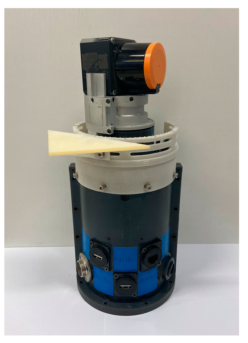
In our method, we define the middle line of the triangular plate according to the center point c. We have also tried to define the middle line by finding the point in point cloud C_tri which is farthest from the rotation axis of the motor shaft (that is, the right-angled vertex of the triangular plate), it turns out that it is less accurate. The reason is obvious, the center point c is calculated based on all the points in point cloud C_tri, while the farthest point is just one point selected from point cloud C_tri. Therefore, the former is more accurate. Moreover, the accuracy of the 2D lidar Hokuyo UST-10LX we use in our prototype is ±40mm. At this level of accuracy, it is necessary to use the average of multiple points instead of a single point to define the middle line of the triangular plate.

(b)

The larger the triangular plate is, the more points are contained in the point cloud C_tri, and the calculation of the center point c is less affected by the accidental error. However, if the size of the triangular plate is too large, it will be inconvenient. The triangular plate installed on our prototype is an isosceles right triangle. The lengths of its three edges are 79.2 mm, 79.2 mm and 112 mm respectively.

(c)

The distance between the triangular plate and the motor shaft should be moderate. If the distance is too close, a part of the triangular plate will be in the blind area of the scanning field and cannot be scanned. If the distance is too far, the beam of 2D lidar will irradiate the triangular plate at a more inclined angle, and the number of the points contained in the point cloud C_tri will be reduced. In our prototype, the distance between the base edge of the isosceles right triangle and the rotation axis of the motor shaft is 54.75 mm.

(d)

Since the center point c is calculated by averaging the 3D coordinates of all the points in the point cloud C_tri, the points in point cloud C_tri should be evenly distributed on the surface of the triangular plate. Therefore, the strip blank area and strip overlap area shown in Figure 5 should be staggered with the point cloud C_tri. This should be considered when determining the installation position of the triangular plate on the prototype. The installation position determines the value of the angle α. In our prototype, α = 30°.

4.2. Calibration of Installation Error of Triangular Plate

In the actual tests, we found the following problems. Due to the installation error of the triangular plate on the prototype, the actual value of the angle α is inconsistent with the expected value (which is 30°), this will make point cloud C_O still have an attitude error. Even seemingly trivial installation errors can result in obvious attitude error of point clouds C_O. Unlike the uncertain attitude error described above, the attitude error here is constant. In order to calibrate this error, we need to find the optimal estimated value α^*. This is an optimization problem. Since this error originates from the installation error of the triangular plate, only one calibration is required for this error, unless the installation position of the triangular plate has been changed, that is, it has been removed and reinstalled. If the installation position of the triangular plate has been changed, the error needs to be calibrated again.

We need to quantify the attitude error of the point cloud C_O. Through the work described above, the point cloud C_O is already known. We collect the 3D point cloud of the conference room once again according to the method described in Figure 1, and perform the following processing on the 3D point cloud. We extract the planes corresponding to the 4 walls of the room, and calculate their unit normal vectors n₁, n₂, n₃, n₄ (this can be done through Point Cloud Library [31]), as shown in Figure 7.

Theoretically, the 3D point cloud in Figure 7 should not be skewed relative to the conference room. However, due to the installation error of the triangular plate, the actual value of the angle α is inconsistent with the expected value, resulting in a slight angular deflection of the 3D point cloud in the direction of Z-axis. This causes the attitude error of the point cloud C_O. This error is denoted as E_atti, and we quantify E_atti by Formula (11)

$$E_{\mathrm{atti}}=\left|{\mathit{n}}_1·\mathit{i}\right|+\left|{\mathit{n}}_3·\mathit{i}\right|+\left|{\mathit{n}}_2·\mathit{j}\right|+\left|{\mathit{n}}_4·\mathit{j}\right|$$

(11)

In Formula (11), we quantify the attitude error E_atti of the point cloud C_O through the sum of the absolute values of the inner product of the unit vector. The vectors n₁, n₂, n₃, n₄ are unit normal vectors extracted from the point cloud C_O, and they correspond to the 4 walls shown in Figure 7. The vectors i and j are unit vectors of the X-axis and Y-axis of the coordinate frame O, respectively. The vectors i and j are fixed because the coordinate frame O is fixed relative to the stationary part of the prototype, the positive direction of X-axis parallel to the front direction of the prototype (see Section 3.2). In Figure 7, we put the prototype in the conference room in a fixed and not-skewed way. Therefore, the coordinate frame O is fixed and not-skewed relative to the conference room.

If there is not any skew for point cloud C_O relative to coordinate frame O, the vectors n₁ and n₃ are perpendicular to the vector i, and the vectors n₂ and n₄ are perpendicular to the vector j, as a result of which, E_atti = 0. While the angular deflection of the 3D point cloud C_O is between −90° and +90°, E_atti increases as the absolute value of the angular deflection increases. Obviously, in the actual situation, the angular deflection of the 3D point cloud C_O cannot exceed the above range.

We denote the skew angle of the point cloud C_O as φ_error, that is, the angular deviation of the point cloud C_O relative to the correct attitude in the direction of Z-axis. If we rotate point cloud C_O by angle φ_error to make it coincide with the correct attitude, then we can make E_atti = 0. Since the vectors n₁, n₂, n₃, n₄ are extracted from the point cloud C_O, while we rotate point cloud C_O, vectors n₁, n₂, n₃, n₄ are also be rotated. We substitute the rotated vectors into Formula (11), and we can get the following formula:

$$f\left({\phi }_{\mathrm{error}}\right)=\left|{\mathit{R}}_{\mathrm{error}}{\mathit{n}}_1·\mathit{i}\right|+\left|{\mathit{R}}_{\mathrm{error}}{\mathit{n}}_3·\mathit{i}\right|+\left|{\mathit{R}}_{\mathrm{error}}{\mathit{n}}_2·\mathit{j}\right|+\left|{\mathit{R}}_{\mathrm{error}}{\mathit{n}}_4·\mathit{j}\right|$$

(12)

where ${\mathit{R}}_{\mathrm{error}}$ is a rotation matrix calculated according to angle φ_error

$${\mathit{R}}_{\mathrm{error}}=\left[\begin{array}{ccc}c({\phi }_{\mathrm{error}})& -s({\phi }_{\mathrm{error}})& 0\\ s({\phi }_{\mathrm{error}})& c({\phi }_{\mathrm{error}})& 0\\ 0& 0& 1\end{array}\right]$$

(13)

It is easy to find that, ideally:

$$f\left({\phi }_{\mathrm{error}}\right)=0$$

(14)

The angle φ_error is numerically equal to the difference between the actual value and the expected value of angle α, that is:

$${\phi }_{\mathrm{error}}=\alpha -30°$$

(15)

where 30° is the expected value of the angle α. Combining Formulas (12), (13), (15), we can change the independent variable of the function $f\left({\phi }_{\mathrm{error}}\right)$ from φ_error to α, that is, function f_cost(α) can be constituted, as shown below:

$$f_{\mathrm{cost}}\left(\alpha \right)=\left|{\mathit{R}}_{\mathrm{error}}{\mathit{n}}_1·\mathit{i}\right|+\left|{\mathit{R}}_{\mathrm{error}}{\mathit{n}}_3·\mathit{i}\right|+\left|{\mathit{R}}_{\mathrm{error}}{\mathit{n}}_2·\mathit{j}\right|+\left|{\mathit{R}}_{\mathrm{error}}{\mathit{n}}_4·\mathit{j}\right|$$

(16)

where ${\mathit{R}}_{\mathrm{error}}$ has been changed to:

$${\mathit{R}}_{\mathrm{error}}=\left[\begin{array}{ccc}c(\alpha -30°)& -s(\alpha -30°)& 0\\ s(\alpha -30°)& c(\alpha -30°)& 0\\ 0& 0& 1\end{array}\right]$$

(17)

It is easy to find that, ideally:

$$f_{\mathrm{cost}}\left(\alpha \right)=0$$

(18)

Next, we need to find the actual value of angle α. This is an optimization problem, our goal is to find α^* through:

$${\alpha }^{*}=argmin{F}_{\mathrm{cost}}(\alpha )$$

(19)

where

$$F_{\mathrm{cost}}(\alpha )=\frac{1}{2}{\displaystyle \sum _{m=1}^{\mathrm{M}}\left(f_{\mathrm{cost}}{\left({\alpha }_m\right)}^2\right)}$$

(20)

In Formula (20), M is the total number of measurements, and m is the serial number of a certain measurement. The optimization requires multiple 3D scans, because it is necessary to eliminate the interference of random factors, so that the actual value of angle α can be estimated more accurately.

We did 50 repeated scans in the highest resolution mode (mode 7, see Table 1) according to the method described in Figure 7, and used these 50 3D point clouds C_O as the input of the optimization algorithm, that is, $\left\{{\mathit{C}}_O^1,{\mathit{C}}_O^2,{\mathit{C}}_O^3,\dots ,{\mathit{C}}_O^{50}\right\}$. The optimized value of angle α is the output of the algorithm. The reason why mode 7 is used is that in lower resolution mode (such as mode 1), the points in point cloud C_tri are sparser, so that the error of the 3D coordinate of the center point c is bigger. The inaccuracy of point c leads to the inaccuracy of angle β. Since the value of the angle α is constant, through Equation (10) we can know that the angle φ_offset inherits the inaccuracy of the angle β, which ultimately leads to the inaccuracy of the attitude of point cloud C_O, as shown in Equations (8) and (9).

Although the attitude of point cloud C_O has been corrected, there are still residual errors remaining. One stems from the above-mentioned inaccuracy of point c, which is particularly obvious in low-resolution mode. The other stems from the constant error of the angle α caused by the installation error, which depends on the accuracy of the installation and has nothing to do with the scanning mode. In low-resolution mode, the former is the main factor. The phenomenon is that the attitude of point cloud C_O obtained from several 3D scans is slightly different. In the high-resolution mode, the latter is the main factor. The phenomenon is that the attitude of the point cloud C_O obtained from several 3D scans is almost the same, but there is a constant difference between the attitude of point cloud C_O and the correct attitude. Here we focus on the latter, and calibrate the installation error of the triangular plate. Therefore, we use the highest resolution mode to collect data as the input of our optimization algorithm, for the purpose of avoiding the above-mentioned first type of error as much as possible, that is, the error caused by low resolution.

In our optimization algorithm, we use the Levenberg–Marquardt method [32,33] to estimate the angle α. Because the initial value and the final optimization result are very close (the installation error is generally small), the initial value is set as α₀ = 30°. Our optimization algorithm is shown in Algorithm A1, which is in Appendix C.

By Algorithm A1, we can estimate the value of angle α, α = 29.3598°. In Equation (10) for the calculation of φ_offset, the value of angle α is replaced from the expected value of 30° to the value estimated by Algorithm A1.

Until now, we can accurately calculate the angle φ_offset between point cloud C_O’ relative to coordinate frame O’ and point cloud C_O relative to coordinate frame O. Since point cloud C_O’ and angle φ_offset are both known, point cloud C_O can be calculated according to Equations (8) and (9). It is accurate both in shape or attitude.

Summarizing our method, in Section 2 and Section 3, we obtained the 3D point cloud C_O’, which has an uncertain attitude error, but no shape error. In Section 4.1, we calibrated the uncertain attitude error of the point cloud C_O’ by using a triangular plate. In Section 4.2, we corrected the installation error of the triangular plate. Through the above steps, we can use our prototype to obtain a 3D point cloud with correct shape and attitude. We have calibrated the matching error between the 2D lidar and the motor at low cost. Unlike the existing methods, we do not need a sensor to measure the rotation angle of the motor shaft, which is costly.

5. Experiments

5.1. Effectiveness Test

5.1.1. Data of Experiments

According to the method described in Figure 7, a total of 70 point clouds were collected, which can be divided into 2 groups, one is without attitude correction, and the other is with attitude correction. In each group, 7 modes of the prototype were tested respectively, and 5 point clouds were collected in each mode.

First, we show the data qualitatively. In Figure 8, the top views of these 70 3D point clouds are listed, which can show the attitude of the 3D point cloud. The red 3D point cloud was obtained without attitude correction (that is, point cloud C_O’), and the blue 3D point cloud was obtained with attitude correction (that is, point cloud C_O).

It can be found from Figure 8 that the attitudes of the 3D point clouds without correction (which are red) are uncertain. This uncertainty exists not only between different modes, but also between different 3D point clouds in the same mode. In comparison, the attitudes of the 3D point clouds with correction (which are blue) are roughly constant. In the following, the attitudes of 3D point clouds will be showed quantitatively by the curves of data.

In order to highlight the strip blank area and strip overlap area of each 3D point cloud, we marked them by a thick orange line. It is the position of the motor shaft when a 3D scanning starts. For the 3D point clouds with attitude correction, although their attitudes are roughly the same, the positions of the thick orange lines relative to the 3D point clouds are not the same. As mentioned above, the thick orange line shows the position of the motor shaft when a rotating 2D lidar starts a 3D scan, that is, the position of the Y’-axis in the coordinate frame O’. Since this position is not constant for each 3D scan, the position of thick orange line relative to the 3D point cloud is different for different 3D point clouds.

Next, we show the data quantitatively. We calculated the angle φ_error of each 3D point cloud in Figure 8 through Equations (12)–(14). It is worth noting that $f\left({\phi }_{\mathrm{error}}\right)=0$ in Formula (14) is under ideal conditions. During data processing, we calculated the φ_error that minimizes $f\left({\phi }_{\mathrm{error}}\right)$ as the result.

The values of angle φ_error of 70 3D point clouds are shown in Figure 9. We used a line chart to make it more intuitive. The horizontal axis is the number of the mode, that is, mode 1 to mode 7 of the prototype. The vertical axis is the value of angle φ_error, its units are degrees. Looking down on a 3D point cloud, if the offset is clockwise relative to the correct attitude, φ_error is positive, while a counterclockwise offset relative to the correct attitude, indicates negative error. The red line corresponds to the 3D point clouds without attitude correction, and the blue line corresponds to the 3D point clouds with attitude correction. For each line, it is divided into 7 segments by 7 modes, and there are 5 sampling points in each mode, which corresponding to 5 3D point clouds collected in this mode.

For the values of angle φ_error of the 5 sampling points in each mode, we calculated the maximum, average and minimum values respectively, as shown in Figure 10.

Through the above experimental data, we can know the following points.

5.1.2. Characteristics of Uncertain Attitude Error

Here, we only considered the sample data without attitude correction. The characteristics of uncertain attitude error were found out.

From mode 1 to mode 7, there is an obvious decreasing trend for the value of the uncertain attitude error. According to Section 2, an important reason for the uncertain attitude error of the 3D point cloud is the uncertain time deviation between the starting time of the 2D lidar and the starting time of the motor). Although the value of this time deviation is uncertain, it changes within a certain range. Therefore, in general, the faster the motor shaft rotates during this time deviation, the larger the attitude error of the 3D point cloud tends to be. The red part of Figure 8, Figure 9 and Figure 10 verify this analysis. From mode 1 to mode 7, the scanning resolution of a rotating 2D lidar is getting higher and higher, and the speed of the motor shaft is getting slower and slower. Therefore, there is a tendency that the attitude error is reduced. However, individual cases that violate this trend still exists. There is a sampling point in the segment corresponding to mode 5 of the red line in Figure 9 (the 22nd point), and its attitude error is much larger than other sampling points in the mode 5 segment, and also much larger than the sampling points in the mode 4 segment. During our tests, cases like this are not unique. This is because although there is a strong correlation between the uncertain attitude error of the 3D point cloud and the speed of the motor shaft, other factors also count. First, the value of the time deviation is uncertain. The response time of the photoelectric switch and the acceleration characteristics of the motor may also have impacts on the uncertain attitude error. We have analyzed this in detail in Section 2.

From mode 1 to mode 7, there is an obvious decreasing trend for the uncertainty of the uncertain attitude error. During the uncertain time deviations, the faster the shaft of the motor rotates, the greater the uncertainty of the time deviation will be transformed into the uncertainty of the attitude of the 3D point cloud. The red part of Figure 10 validates this analysis, which shows the maximum, average, and minimum attitude errors of the 5 3D point cloud collected in each mode. Obviously, there is an overall trend that the higher the resolution of the scanning mode, the closer these three values are, which means that the uncertainty of the uncertain attitude error turns smaller.

5.1.3. Characteristics of Our Algorithm

Here, we only considered the sample data with attitude correction. The characteristics of our algorithm were found out.

It can be seen from the blue part of Figure 9 and Figure 10 that for the high-resolution mode, the attitude error of the corrected 3D point cloud is smaller and more certain. For the low-resolution mode, the attitude error of the corrected 3D point cloud is larger and more uncertain. The reason has been analyzed in Section 4.2, because the points in point cloud C_tri obtained in the low-resolution mode are relatively sparse, so that the calculated center point c has a large error. The error is shown in two points, one is that the calculated value of center point c has a large deviation from the true value, the other is that the calculated value of center point c is greatly uncertain in each 3D scan. The above two points will lead to a large and uncertain error of angle β, because the angle β is calculated according to the 3D coordinates of the point c. As a result, a large and uncertain error of angle φ_offset is caused. This can be seen from Formula (10). Where α is a constant value. According to Formulas (8) and (9), this can finally result in a large and uncertain attitude error of the point cloud C_O.

5.1.4. Effectiveness of Our Algorithm

Here, we compared the sample data without attitude correction and the sample data with attitude correction to evaluate the effectiveness of our algorithm.

It can be seen from the value of φ_error that the attitude error is eliminated by our algorithm. This can be clearly seen from Figure 8, Figure 9 and Figure 10, the 3D point clouds without attitude correction (which is red) are obviously skew, and there are an obvious deviations between their φ_error and 0, while the attitudes of the 3D point clouds with attitude correction (which is blue) are correct, and their φ_error approach 0.

It can be seen from the uncertainty of φ_error that, in general, in the same mode, the uncertainty of φ_error of a 3D point cloud with attitude correction is smaller than that of a 3D point cloud without attitude correction (as shown in Figure 10). Comparing the red part and blue part of Figure 10, our algorithm reduces the uncertainty of φ_error, especially in low-resolution mode. In high-resolution mode, our algorithm does not show obvious performance in reducing the uncertainty of φ_error. After all, in high-resolution mode, the uncertainty of the attitude of the 3D point cloud is very small—even without attitude correction. However, mutation point which is similar to the 22nd point of the red line showed in Figure 9 cannot be excluded. Our algorithm can deal with this situation.

Our algorithm is effective, whether it is to reduce the attitude error of the 3D point cloud, or to reduce the uncertainty of the 3D point cloud attitude. As for whether the accuracy of our algorithm can meet the application requirements, we will analyze it below.

5.2. Accuracy Test and Application Evaluation

In this section, we evaluated whether the accuracy of our method can meet the requirements of the application. We used the 3D mapping of indoor autonomous mobile robots as the actual application, because a rotating 2D lidar is widely used in the 3D mapping of indoor mobile robots [17,34,35,36], and the 2D lidar Hokuyo UST-10LX [30] used in our prototype is a product mainly used for indoor. In this application, the main negative effect of the attitude error of the 3D point cloud is to make the robot navigate in the wrong direction, thereby increasing the risk of crashing the wall. The variation curve of the mapping error E_map with distance d in 7 modes is shown in Figure 11. The mapping error E_map is calculated by the following formula

$$E_{\mathrm{map}}=d·\tan ({\phi }_{\mathrm{error}})$$

(21)

There are 7 graphs in Figure 11, which correspond to the 7 scan modes of the prototype. The horizontal axis of the graph is the distance d, its units are meters. The vertical axis of the graph is the mapping error E_map, its units are millimeters. The maximum range of the horizontal axis d is 10 m, which is the range of the 2D lidar we used in our prototype. The three curves in each graph are the variation curve of E_map with distance d calculated according to the maximum, average and minimum values of angle φ_error, respectively. The area between the top curve and the bottom curve represents the variation range of the attitude error of the 3D point cloud in this mode.

We took ±50 mm as a standard, and marked the corresponding d while the mapping error E_map of each mode is limited within ±50 mm in Figure 11. Even in mode 1, which has the lowest accuracy, the mapping error E_map can be limited within ±50 mm at d = 2.2996 m. In mode 7, the mapping error E_map at the measuring range d = 10 m can be limited within ±50 mm. For 3D mapping of indoor autonomous mobile robots, a mapping error of ±50 mm is acceptable. After all, the accuracy of the 2D lidar Hokuyo UST-10LX used in our prototype is ±40 mm [30]. Moreover, after the robot has approached a target (such as a door), the rotating 2D lidar mounted on it can 3D scan again to refresh the 3D map. According to Formula (21), the mapping error E_map of this target will be reduced because the distance is closer.

The above analysis has verified that the accuracy of our method can meet the requirements of 3D mapping of indoor autonomous mobile robots.

6. Conclusions

For a rotating 2D lidar, the inaccurate matching between the 2D lidar and the motor is an important cause of the shape and attitude error of the 3D point cloud. To solve this problem, existing methods need to synchronize the 2D lidar data and the motor shaft by measuring the angle position of the motor shaft. To measure the angle position of the motor shaft, either a complicated and expensive servo system with absolute positioning function is required, or the motor needs to be equipped with a precise angular displacement sensor, such as an absolute encoder. This will greatly increase the cost.

Our method eliminates the shape and attitude error of the 3D point cloud caused by the inaccurate matching between the 2D lidar and the motor, without using a servo system or encoder. First, we modified the sequence between the motor and the 2D lidar to make the motor start working earlier and stop working later than the 2D lidar, so that the shape of the 3D point cloud is no longer affected by the acceleration and deceleration of the motor, a 3D point cloud with correct shape can be obtained. Next, we eliminated the uncertain error of the attitude of the 3D point cloud through a triangular plate fixed on the prototype. Finally, we calibrated the installation error of the triangular plate by using Levenberg–Marquardt method. We verified the effectiveness and accuracy of our method by experiments. The results show that the collected 3D point cloud can meet the requirements of 3D mapping of an indoor autonomous mobile robot. Through our work, while reducing the cost, the accuracy is ensured. Our work provides a new idea for the cost reduction of a rotating 2D lidar.

Our method can not only calibrate the matching error between the 2D lidar and the motor, but also partially calibrate the installation error between the 2D lidar and the motor shaft. The installation error is 6-DOF, containing a 3-DOF translation and 3-DOF rotation [4]. The direction of one of the rotation errors is the same as the rotation direction of the motor shaft. It will not cause the shape error of the 3D point cloud, but it will cause the attitude error of the 3D point cloud. Due to its characteristic that it will not cause the distortion in shape of the 3D point cloud, it is difficult to calibrate it [1,5], while our method can calibrate it.

As for future work, we have noticed that the real-time performance of a rotating 2D lidar is very poor, and its 3D scanning frequency is often not higher than 1Hz. Therefore, when a rotating 2D lidar is scanning, the movement of the platform carrying the rotating 2D lidar will cause the distortion of the 3D point cloud [24,25,27]. Therefore, for a rotating 2D lidar, it is not enough to obtain an accurate 3D point cloud in static state, it is necessary to study how to eliminate the distortion of the 3D point cloud in motion state. Our follow-up plan is to combine our method with an algorithm that calibrates the distortion of the 3D point cloud in a dynamic environment. We will try to collect an accurate 3D point cloud (which is accurate both in shape and attitude) in a dynamic environment, by using a low-cost rotating 2D lidar which does not require an angular sensor to measure the angle of motor shaft.

References

1. Morales, J.; Martinez, J.L.; Mandow, A.; Reina, A.J.; Pequenoboter, A.; Garciacerezo, A. Boresight Calibration of Construction Misalignments for 3D Scanners Built with a 2D Laser Rangefinder Rotating on Its Optical Center. Sensors 2014, 14, 20025–20040. [Google Scholar] [CrossRef] [PubMed] [Green Version]
2. Morales, J.; Martinez, J.L.; Mandow, A.; Pequenoboter, A.; Garciacerezo, A. Design and development of a fast and precise low-cost 3D laser rangefinder. In Proceedings of the International Conference on Mechatronics, Istanbul, Turkey, 13–15 April 2011; pp. 621–626. [Google Scholar]
3. Wulf, O.; Wagner, B. Fast 3d scanning methods for laser measurement systems. In International Conference on Control Systems and Computer Science; Editura Politehnica Press, 2003; Available online: https://www.researchgate.net/publication/228586709_Fast_3D_scanning_methods_for_laser_measurement_systems (accessed on 6 January 2021).
4. Kang, J.; Doh, N.L. Full-DOF Calibration of a Rotating 2-D LIDAR with a Simple Plane Measurement. IEEE Trans. Robot. 2016, 32, 1245–1263. [Google Scholar] [CrossRef]
5. Gao, Z.; Huang, J.; Yang, X.; An, P. Calibration of rotating 2D LIDAR based on simple plane measurement. Sens. Rev. 2019, 39, 190–198. [Google Scholar] [CrossRef]
6. Alismail, H.; Browning, B. Automatic Calibration of Spinning Actuated Lidar Internal Parameters. J. Field Robot. 2015, 32, 723–747. [Google Scholar] [CrossRef]
7. Zeng, Y.; Yu, H.; Dai, H.; Song, S.; Lin, M.; Sun, B.; Jiang, W.; Meng, M.Q.H. An Improved Calibration Method for a Rotating 2D LIDAR System. Sensors 2018, 18, 497. [Google Scholar] [CrossRef] [PubMed] [Green Version]
8. Martinez, J.L.; Morales, J.; Reina, A.J.; Mandow, A.; Pequeno-Boter, A.; Garcia-Cerezo, A. Construction and Calibration of a Low-Cost 3D Laser Scanner with 360 degrees Field of View for Mobile Robots. In Proceedings of the 2015 IEEE International Conference on Industrial Technology (ICIT), Seville, Spain, 17–19 March 2015; pp. 149–154. [Google Scholar]
9. Murcia, H.F.; Monroy, M.F.; Mora, L.F. 3D Scene Reconstruction Based on a 2D Moving LiDAR. In International Conference on Applied Informatics; Springer: Cham, Switzerland, 2018. [Google Scholar]
10. Olivka, P.; Krumnikl, M.; Moravec, P.; Seidl, D. Calibration of Short Range 2D Laser Range Finder for 3D SLAM Usage. J. Sens. 2016, 2016. [Google Scholar] [CrossRef] [Green Version]
11. Oberlaender, J.; Pfotzer, L.; Roennau, A.; Dillmann, R. Fast Calibration of Rotating and Swivelling 3-D Laser Scanners Exploiting Measurement Redundancies. In Proceedings of the 2015 IEEE/RSJ International Conference on Intelligent Robots and Systems, Hamburg, Germany, 28 September–2 October 2015; pp. 3038–3044. [Google Scholar]
12. Kurnianggoro, L.; Hoang, V.-D.; Jo, K.-H. Calibration of Rotating 2D Laser Range Finder Using Circular Path on Plane Constraints. In New Trends in Computational Collective Intelligence; Camacho, D., Kim, S.W., Trawinski, B., Eds.; Springer: Cham, Switzerland, 2015; Volume 572, pp. 155–163. [Google Scholar]
13. Kurnianggoro, L.; Hoang, V.-D.; Jo, K.-H. Calibration of a 2D Laser Scanner System and Rotating Platform using a Point-Plane Constraint. Comput. Sci. Inf. Syst. 2015, 12, 307–322. [Google Scholar] [CrossRef]
14. Pfotzer, L.; Oberlaender, J.; Roennau, A.; Dillmann, R. Development and calibration of KaRoLa, a compact, high-resolution 3D laser scanner. In Proceedings of the IEEE International Symposium on Safety, Hokkaido, Japan, 27–30 October 2014. [Google Scholar]
15. Lin, C.C.; Liao, Y.D.; Luo, W.J. Calibration method for extending single-layer LIDAR to multi-layer LIDAR. In Proceedings of the 2013 IEEE/SICE International Symposium on System Integration (SII), Kobe, Japan, 15–17 December 2013. [Google Scholar]
16. Ueda, T.K.H.; Tomizawa, T. Mobile SOKUIKI Sensor System-Accurate Range Data Mapping System with Sensor Motion. In Proceedings of the 2006 International Conference on Autonomous Robots and Agents, Palmerston North, New Zealand, 12–14 December 2006. [Google Scholar]
17. Nagatani, K.; Tokunaga, N.; Okada, Y.; Yoshida, K. Continuous Acquisition of Three-Dimensional Environment Information for Tracked Vehicles on Uneven Terrain. In Proceedings of the IEEE International Workshop on Safety, Sendai, Japan, 21–24 October 2008. [Google Scholar]
18. Matsumoto, M.; Yuta, S. 3D laser range sensor module with roundly swinging mechanism for fast and wide view range image. In Proceedings of the Multisensor Fusion & Integration for Intelligent Systems, Salt Lake City, UT, USA, 5–7 September 2010. [Google Scholar]
19. Walther, M.; Steinhaus, P.; Dillmann, R. A foveal 3D laser scanner integrating texture into range data. In Proceedings of the International Conference on Intelligent Autonomous Systems 9-ias, Tokyo, Japan, 7–9 March 2006. [Google Scholar]
20. Raymond, S.; Nawid, J.; Waleed, K.; Claude, S. A Low-Cost, Compact, Lightweight 3D Range Sensor. In Proceedings of the Australasian Conference on Robotics and Automation; Available online: https://www.researchgate.net/publication/228338590_A_Low-Cost_Compact_Lightweight_3D_Range_Sensor (accessed on 6 January 2021).
21. Dias, P.; Matos, M.; Santos, V. 3D Reconstruction of Real World Scenes Using a Low-Cost 3D Range Scanner. Comput.-Aided Civ. Infrastruct. Eng. 2006, 21, 486–497. [Google Scholar] [CrossRef]
22. Nasrollahi, M.; Bolourian, N.; Zhu, Z.; Hammad, A. Designing LiDAR-equipped UAV Platform for Structural Inspection. In Proceedings of 34th International Symposium on Automation and Robotics in Construction; IAARC Publications, 2018; Available online: https://www.researchgate.net/publication/328370814_Designing_LiDAR-equipped_UAV_Platform_for_Structural_Inspection (accessed on 6 January 2021).
23. Bertussi, S. Spin_Hokuyo—ROS Wiki. Available online: http://wiki.ros.org/spin_hokuyo (accessed on 13 October 2020).
24. Bosse, M.C.; Zlot, R.M. Continuous 3D scan-matching with a spinning 2D laser. In Proceedings of the IEEE International Conference on Robotics & Automation, Kobe, Japan, 12–17 May 2009. [Google Scholar]
25. Zheng, F.; Shibo, Z.; Shiguang, W.; Yu, Z. A Real-Time 3D Perception and Reconstruction System Based on a 2D Laser Scanner. J. Sens. 2018, 2018, 1–14. [Google Scholar] [CrossRef]
26. Almqvist, H.; Magnusson, M.; Lilienthal, A.J. Improving Point Cloud Accuracy Obtained from a Moving Platform for Consistent Pile Attack Pose Estimation. J. Intell. Robot. Syst. 2014, 75, 101–128. [Google Scholar] [CrossRef]
27. Zhang, J.; Singh, S. LOAM: Lidar Odometry and Mapping in Real-time. In Robotics: Science and Systems; 2014; Available online: https://www.researchgate.net/publication/311570125_LOAM_Lidar_Odometry_and_Mapping_in_real-time (accessed on 6 January 2021).
28. Zhang, T.; Nakamura, Y. Moving Humans Removal for Dynamic Environment Reconstruction from Slow-Scanning LIDAR Data. In Proceedings of the 2018 15th International Conference on Ubiquitous Robots, Honolulu, HI, USA, 26–30 June 2018; pp. 449–454. [Google Scholar]
29. David, Y.; Kent, W. “Sweep Diy 3d Scanner Kit” Project. Available online: https://www.servomagazine.com/magazine/article/the-multi-rotor-hobbyist-scanse-sweep-3d-scanner-review? (accessed on 16 October 2020).
30. Hokuyo UST-10/20LX. Available online: https://www.hokuyo-aut.co.jp/search/single.php?serial=16 (accessed on 16 October 2020).
31. Point Cloud Library. Available online: https://pointclouds.org/ (accessed on 16 October 2020).
32. More, J.J. The Levenberg-Marquardt algorithm: Implementation and theory. In Lecture Notes in Mathematicsl; Springer: Berlin/Heidelberg, Germany, 1978; Volume 630. [Google Scholar]
33. Madsen, K.; Nielsen, H.B.; Tingleff, O. Methods for Non-Linear Least Squares Problems, 2nd ed.; Informatics and Mathematical Modelling (IMM), Technical University of Denmark (DTU): Lyngby, Denmark, 2004. [Google Scholar]
34. Ricaud, B.; Joly, C.; de La Fortelle, A. Nonurban Driver Assistance with 2D Tilting Laser Reconstruction. J. Surv. Eng. 2017, 143. [Google Scholar] [CrossRef]
35. Yan, F.; Zhang, S.; Zhuang, Y.; Tan, G. Automated indoor scene reconstruction with mobile robots based on 3D laser data and monocular visual odometry. In Proceedings of the 2015 IEEE International Conference on CYBER Technology in Automation, Control, and Intelligent Systems (CYBER), Shenyang, China, 8–12 June 2015. [Google Scholar]
36. Colas, F.; Mahesh, S.; Pomerleau, F.; Liu, M.; Siegwart, R. 3D path planning and execution for search and rescue ground robots. In Proceedings of the IEEE/RSJ International Conference on Intelligent Robots & Systems, Tokyo, Japan, 3–7 November 2013. [Google Scholar]
Figure 1. The shape error and attitude error of the 3D point cloud: (a) a photo of the environment for collecting the 3D point cloud; (b) top view of a 3D point cloud collected by a rotating 2D lidar; (c) top view of another 3D point cloud collected by a rotating 2D lidar.
Applsci 11 00913 g001
Figure 2. Improved action sequence of the 2D lidar and stepper motor.
Applsci 11 00913 g002
Figure 3. A photo of our prototype. The 2D lidar Hokuyo UST-10LX is installed on a rotating unit, and a triangular plate is used to calibrate the attitude error of the 3D point cloud.
Applsci 11 00913 g003
Figure 4. Three Cartesian coordinate frames. The coordinate frame of the 2D lidar (L) is shown in green, the coordinate frame of rotating unit before attitude correction (O’) is shown in blue, and the coordinate frame of rotating unit after attitude correction (O) is shown in red.
Applsci 11 00913 g004
Figure 5. The scanning sector of the 2D lidar does not coincide with the rotation axis of the motor shaft. They are parallel to each other, and the distance between them is 13.9 mm. This design can collect the 3D point cloud with a mark, which can roughly show the position of the motor shaft at the moment a 3D scan is started, that is, the position of the Y’-axis of coordinate frame O’-X’Y’Z’.
Applsci 11 00913 g005
Figure 6. In order to extract the point cloud Ctri from the point cloud CO’, we define a special area, which is shown in blue.
Applsci 11 00913 g006
Figure 7. Extract the planes corresponding to the 4 walls of the conference room, and calculate their unit normal vector. (a) The top view of the room, where the red bold line is the walls used to extract the planes. Our selection criterion is as follows. The area of the walls should be large so as to facilitate the extraction of the planes. Besides, walls with windows should be avoided, because irregularly shaped curtains may interfere with the extraction of the planes; (b) the 3D point cloud of the conference room, from which we extracted the planes corresponding to 4 walls. We marked them with different colors to distinguish them. There are 6 vectors in (b), where the vectors n1, n2, n3, n4 are the unit normal vectors of the 4 planes, and the vectors i and j are the unit normal vectors of X-axis and Y-axis of coordinate frame O.
Applsci 11 00913 g007
Figure 8. Top views of 70 3D point clouds.
Applsci 11 00913 g008aApplsci 11 00913 g008b
Figure 9. The values of angle φerror of 70 3D point clouds.
Applsci 11 00913 g009
Figure 10. The maximum, average, and minimum values of angle φerror of 5 sampling points in each mode.
Applsci 11 00913 g010
Figure 11. Variation curve of mapping error with distance in 7 modes.
Applsci 11 00913 g011