Abstract
Case-based intelligent fault diagnosis methods of rotating machinery can deal with new faults effectively by adding them into the case library. However, case-based methods scarcely refer to automatic feature extraction, and k-nearest neighbor (KNN) commonly required by case-based methods is unable to determine the nearest neighbors for different testing samples adaptively. To solve these problems, a new intelligent fault diagnosis method of rotating machinery is proposed based on enhanced KNN (EKNN), which can take advantage of both parameter-based and case-based methods. First, EKNN is embedded with a dimension-reduction stage, which extracts the discriminative features of samples via sparse filtering (SF). Second, to locate the nearest neighbors for various testing samples adaptively, a case-based reconstruction algorithm is designed to obtain the correlation vectors between training samples and testing samples. Finally, according to the optimized correlation vector of each testing sample, its nearest neighbors can be adaptively selected to obtain its corresponding health condition label. Extensive experiments on vibration signal datasets of bearings are also conducted to verify the effectiveness of the proposed method.
1. Introduction
In recent decades, rotating machineries have become increasingly complicated, and have been applied to many more fields to meet requirements from both social and economic developments [1,2]. Meanwhile, their automation has also been increasing continuously, and they both put much more demand on machine reliability and stability [3]. Particularly, their rotating transmission parts are more prone to faults since they always work under poor working conditions, which are more likely to trigger much bigger machine operation impacts or even result in catastrophes [4,5]. Hence, many researchers devote great efforts to their fault prognosis and diagnosis investigation [6]. Recently, with the advent of deep learning and development of data collection, storage and computation technologies, data-driven fault diagnosis has attracted increased attention for its lower requirement of expertise in the fault diagnosis stage [7]. Among various data sources, vibration signal contains much principal information of machine health conditions and has been widely used in data-driven fault diagnosis.
Accordingly, to make full use of the mechanical big data in fault diagnosis, there are two main categories of methods. One category of methods trains networks for fault diagnosis utilizing big data, where the training data would be dumped in application and only the optimized network parameters would be stored [8,9]. Motivated from this concept, a variety of diagnosis methods have been developed and applied. Lei et al. [10] developed an intelligent fault diagnosis network characterized by adopting sparse filtering (SF) [11] in feature extraction and further utilizing softmax regression in feature classification. Inspired by the powerful feature extraction capability of SF, its variants are proposed to extract more fault-sensitive features [12,13]. Wen et al. proposed a convolution neural network (CNN) based on two-dimensional images obtained from vibration signals through a signal processing method [14]. Jia et al. [15] constructed a deep neural network (DNN) based on stacked autoencoders (SAE) using frequency spectra of vibration signals as inputs. Liu et al. [16] constructed a novel CNN which can take vibration signals as inputs directly. For automatic fault feature extraction, many other methods based on machine learning are also proposed [17,18,19]. Zhao et al. gave a comprehensive survey of recent work in [20]. These methods are based on automatic feature extraction. Since only the optimized network parameters are stored in their testing stage, they fall into the category of parameter-based fault diagnosis methods here.
The other category of fault diagnosis methods is case-based methods. They are also data-driven methods which store samples and adopt them in the testing stage. These methods adopt a more conservative method, which first measures the similarity between the testing and training samples and then selects the most similar training samples in fault diagnosis [21]. Generally, these methods use case-based reasoning (CBR) [22] techniques to a certain degree. CBR is an analogical reasoning method inspired by the human mind, and uses original cases to obtain final solutions via similarity evaluation between the new case and the original cases [23]. These kinds of methods are referred to as case-based methods here. Although parameter-based methods seem more popular recently, the development of storing and computation techniques also brings about many case-based fault diagnosis methods. To date, various case-based methods have been proposed and have found wide applications [24,25,26].
Parameter-based and case-based methods, although effective, both have some disadvantages as well. Parameter-based methods take advantage of deep learning, but they simply treat the optimized structure as the only decision basis, and dump the informative samples [27,28]. When the network is trained, only the structure parameters are stored. However, when a new kind of fault appears, it is not easy to obtain a new network suitable for the original faults and the new one. As for case-based methods, they store the samples, and when the samples of new faults appear, we only need to add them into the data library, that is, the new fault can also be diagnosed. However, case-based methods also have some shortcomings. First, they rely on previous fault diagnosis cases. Compared with parameter-based methods, they pay less attention to feature extraction [29,30,31]. However, it is validated that feature extraction is essential and helpful for fault-sensitive feature extraction, which accounts for why parameter-based methods are more popular in recent years. Second, most case-based methods inevitably need k-nearest neighbor (KNN) [32,33] in classification. Although KNN is a well-known effective and simple classification method, KNN-based methods inevitably need to locate k nearest neighbors in each testing sample diagnosis, which is mainly based on similarity evaluation and is usually quite expensive [34,35].
Aiming to overcome these shortcomings, we propose a new method called enhanced k-nearest neighbor (EKNN) to intelligently diagnose faults of rotating machineries; it combines the advantage of both parameter-based methods and case-based classification methods. In the second stage, a powerful and efficient sparse feature extraction method is applied to extract discriminative features. In the third stage, a novel reconstruction method is developed to obtain the correlation vector between each testing sample and training samples, which automatically points out the nearest neighbors of each testing sample in the training dataset. In the fourth stage, similar to the common KNN-based method, the final classification result of the testing sample is obtained via the voting results of its nearest neighbors. Compared with existing methods, there are mainly three aspects of innovation in our methods.
- (1)
- For bearing fault diagnosis, a fourth-stage novel data-driven fault diagnosis method is developed, which takes advantage of both parameter-based and case-based methods and addresses the shortcomings in common KNN-based fault diagnosis methods. As regards feature extraction, it uses a powerful sparse feature extraction method to extract discriminative features. In its feature classification part, inspired by sparse coding [36], a novel method called EKNN is proposed to realize automatic nearest neighbor location.
- (2)
- For EKNN, it can also take advantage of the training dataset in the testing stage, retaining the advantages of case-based methods in feature classification. With the help of the training dataset, when new faults occur, EKNN can fuse the related data to train and obtain a new diagnosis network suitable for all faults.
- (3)
- To solve the nearest neighbor location problem in the common KNN-based fault diagnosis method, a reconstruction method is proposed in EKNN for the testing sample nearest to neighbor determination. It attempts to obtain the correlation vector of each testing sample in the testing sample reconstruction utilizing training samples, which distinguishes it from existing methods.
2. Principal Knowledge
2.1. Sparse Filtering
SF is a two-layer unsupervised feature extraction network seeking to optimize the feature matrix sparsity [11], which is able to extract discriminative features instead of principal components of inputs. Suppose the input matrix is , and is the i-th column instance in Z. It optimizes the sparsity through the following three steps:
- (1)
- Feature extraction via Equation (1);
- (2)
- Feature matrix normalization with L2 norm by Equation (2);
- (3)
- Optimization via minimizing L1 norm in the objective function, namely, Equation (3), to maximize the sparsity of . The weight matrix updating of SF can be derived by backpropagation step-by-step.
2.2. Sparse Coding
Sparse coding is inspired by the biological brain network, and its target is reconstructing the input vector. Its core assumption is that the input vector can be approximated by linear fitting via some of the existing base vectors. Suppose the input matrix is X, and is the i-th target vector in it; V is the dictionary matrix and is the i-th column base; U is coefficient matrix of X, where is the i-th coefficient vector of , which reconstructs from the dictionary matrix U. It is worth mentioning that the amount of base vector in V is much larger than the input dimension, which means the dictionary matrix is over-complete. Correspondingly, the objective function of sparse coding can be formed as Equation (4).
where the first term is the reconstruction term, and the second term is the regular term for coefficient matrix. It means that each input vector is only composed of the several bases in V; therefore, the coefficient matrix U is bound to be sparse and encouraged to be sparse by minimizing the L1 norm of each coefficient vector here.
3. Proposed Method
For rotating machine fault diagnosis, we propose a new fault diagnosis method called enhanced k-nearest neighbor (EKNN), which tries to combine both the advantages of parameter-based and case-based fault diagnosis methods. Generally, the powerful and automatic feature extraction capability of parameter-based fault diagnosis methods is adopted in EKNN first, and then the case-based classification process is adopted in the feature classification stage of EKNN.
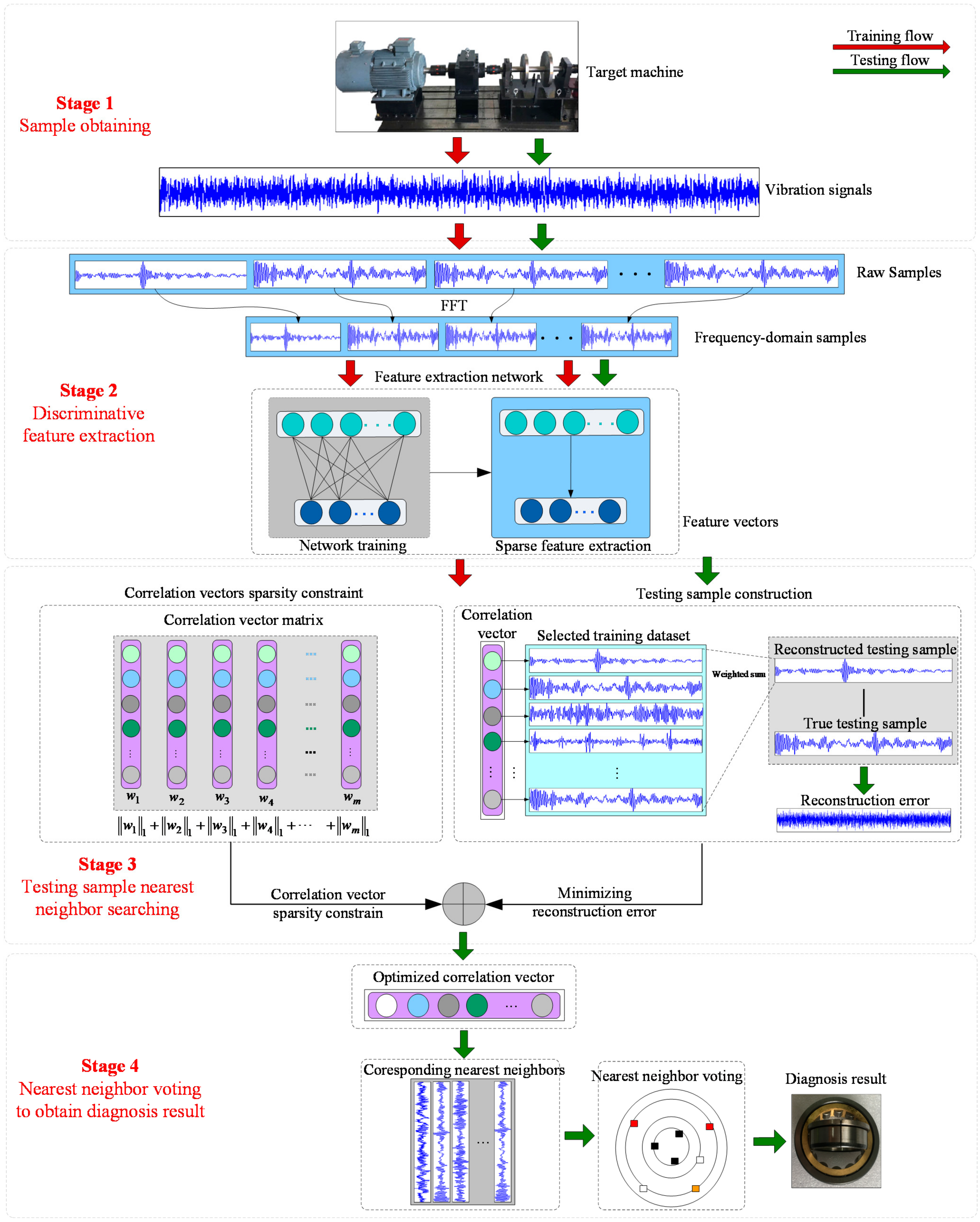
Meanwhile, in order to address the inherent shortcoming of KNN, which is widely-used in case-based fault diagnosis methods, we also propose a novel solution. First, the global search throughout the whole training set is always required to locate k nearest neighbors in KNN, which is cost expensive and laborious. Hence, a new method based on sparse coding and KNN is proposed for feature classification. It can effectively overcome shortcomings by combining sparse coding and the similarity matrix to reconstruct each testing sample from the limited training dataset in order to obtain the correlation vector of each testing sample. After the correlation vector is obtained, the proposed method can determine the nearest neighbors automatically. The proposed EKNN is composed of four stages, and their details are as follows. The flowchart of the proposed method is shown in Figure 1.

Figure 1.
The flowchart of the proposed method.
3.1. Stage 1: Sample Obtaining
In this stage, the vibration signals of various health conditions are acquired from the target machine first. Then, samples of each health condition are obtained from their corresponding vibration signals separately, as shown in Figure 1. In testing, the testing samples are also acquired similarly. Suppose the training dataset is , where is the i-th sample in Z, and is the label of .
3.2. Stage 2: Discriminative Feature Extraction
This stage makes use of the powerful and automatic feature extraction capability of parameter-based methods to obtain fault-sensitive features from time-domain sample for further feature classification. Generally, the features are extracted through two steps.
First, FFT is applied in to obtain its corresponding frequency-domain sample , and all frequency-domain samples compose the training dataset .
Second, the sparse filtering (SF) is applied to the training dataset X to extract discriminative features, which is a two-layer unsupervised network aiming to extract discriminative features of each input. The L-BFGS [37] algorithm is used to optimize the network.
Finally, with the optimized parameter matrix , can be transformed to its feature vector . Additionally, it is also observed in our experiments that the samples transformed by SF can be both quite discriminative and consistent, which means that feature vectors of all samples can be quite similar and activated in the same elements. This property would be likely to make further testing sample reconstruction-based nearest neighbor location more robust.
3.3. Stage 3: Nearest Neighbor Searching
With the training feature dataset, we can find the nearest neighbor search process. To find the nearest neighbors of each testing sample automatically, a new method based on sparse coding and L2 norm is developed. Suppose the training dataset is and testing dataset is , where , and are the input dimension, number of training samples and number of testing samples, respectively.
In the proposed method, the testing samples are reconstructed using the training samples to obtain a correlation matrix . This minimizes the error between Z and WX, namely, the reconstructed testing sample, where is the column correlation vector between the i-th testing sample and . Here, the reconstruction error is evaluated by least square loss, so the reconstruction process can be formed as the first term of Equation (5).
Meanwhile, in this reconstruction process, as the training dataset is always over-complete, the sparsity of each correlation vector is also constrained by minimizing the L1 norm of each correlation vector in the second term of Equation (5). Consequently, some elements of the correlation vector can also be constrained to zero, which is convenient for further nearest neighbor location, where is the regular parameter for importance weight between testing sample reconstruction and the sparsity of W.
Furthermore, it is also found in our experiments that for nearest neighbor location, we need to maximize the correlation between each testing sample and training samples from the same health condition. Hence, similarity correlations between samples are also constrained in the third term of Equation (5), where is also a regular parameter similar to , and L is the similarity matrix between samples, which is calculated by common heat kernel.
In optimization, this algorithm can be optimized via the common L-BFGS method [36], and finally a correlation matrix W is obtained, where is the correlation vector between the training samples and the j-th testing sample, and is j-th element of . Correspondingly, the nearest neighbors of testing sample can be located by listing the elements of in descending order, and the training samples falling on their first c elements are the nearest neighbors, where c is the health condition number.
Through this process, the nearest neighbors can be determined adaptively for different testing samples. Meanwhile, as the sparsity of correlation vectors is also taken into consideration by fusing L1 norm into this process, its nearest neighbor location is more precise.
3.4. Stage 4: Nearest Neighbor Voting to Obtain Diagnosis Result
This stage is similar to common operation in KNN, which classifies the testing samples through the voting results of the nearest neighbors obtained in stage 4, and we can obtain the predicted health condition label of the target testing sample easily.
For the proposed method, when new faults occur in the target machines, as the case-based method preserves the training samples, the new fault samples can be added into existing training dataset to train the feature extraction part of EKNN again, which learns to diagnose them.
The proposed method combines discriminative feature extraction with a training-free feature classification framework in the existing intelligent fault diagnosis field. It is distinct from the traditional fault diagnosis method because it can automatically diagnose the faults of machineries based on the discriminative feature. In addition, as we can see from stages 1–4, each stage of EKNN can be trained separately or needs no training, which means it has low training cost and low overfitting risk compared with fault diagnosis methods based on deep learning.
4. Fault Diagnosis Case Investigation Utilizing the Proposed EKNN
4.1. Dataset Description
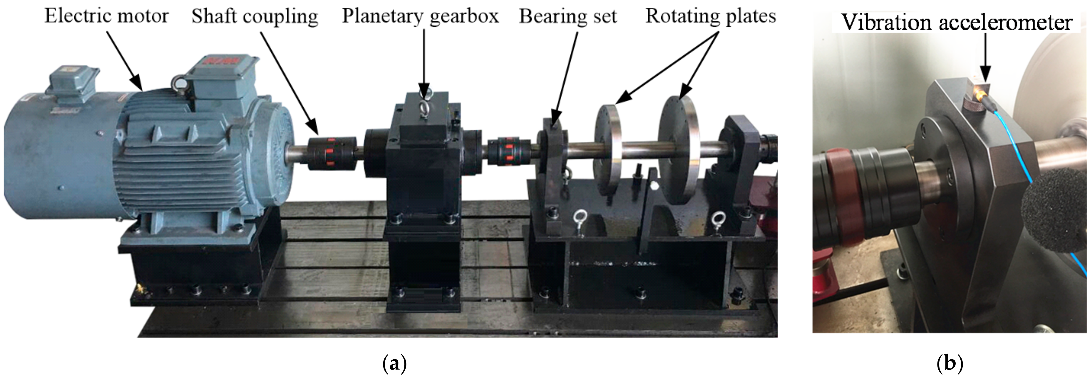
The experiments were carried out on the vibration signals collected from the test rig, and the details are shown in Figure 2. The components include an electric motor, a shaft coupling, a planetary gearbox, a bearing, two rotating plates and a bearing. To acquire the vibration signals, a vibration accelerometer was set on the bearing set between planetary gearbox and rotating plates, and the sampling frequency was 12.8 kHz. Here, the bearings with faults were processed and set in the location of last bearing. Entirely, 10 health conditions are designed:
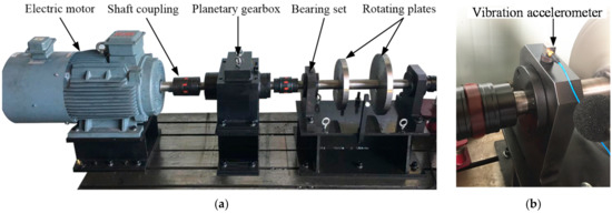
Figure 2.
The details of the test rig: (a) the main components of the testing rig; (b) the location of the vibration accelerometer.
- (1)
- Normal condition, denoted as NO;
- (2)
- Three inner race faults with different fault severities (0.2, 0.6 and 1.2 mm), denoted as IF02, IF06 and IF12, respectively;
- (3)
- Three outer race faults with different fault severities (0.2, 0.6 and 1.2 mm), denoted as OF02, OF06 and OF12, respectively;
- (4)
- Three roller faults with different fault severities (0.2, 0.6 and 1.2 mm), denoted as BF02, BF06 and BF12, respectively.
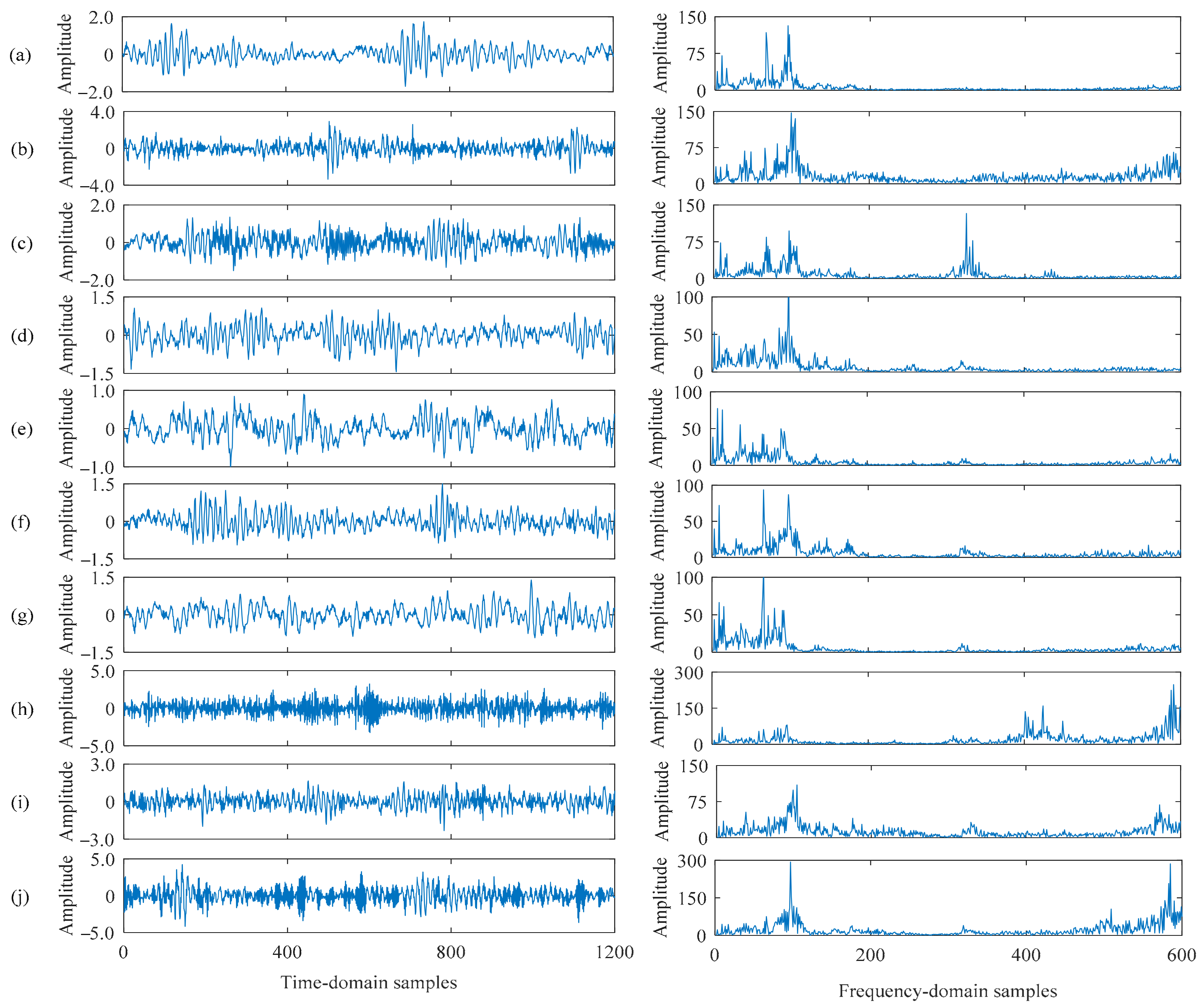
For each vibration signal of each health condition, 400 samples were obtained, and each sample contained 2000 data points; therefore, the whole dataset was composed of 4000 time-domain samples. For network training, 2000 samples were randomly selected, and the rest were used in testing. For clarity, the time-domain samples and their corresponding frequency-domain forms are shown in Figure 3.
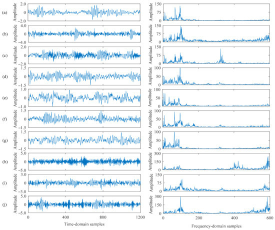
Figure 3.
Time-domain and frequency-domain samples from different health conditions. (a): NO, (b): IF02, (c): IF06, (d): IF12, (e): OF02, (f): OF06, (g): OF12, (h): BF02, (i): BF06, (j): BF12
4.2. Parameter Tuning and Sensitivity Investigation
The proposed method also has three parameters needing manual tuning:
- (1)
- The feature dimension N1 in the feature layer of SF;
- (2)
- The regular parameter ρ1 for L1 norm in Stage 3;
- (3)
- The regular parameter ρ2 for similarity evaluation in stage 3.
Here, is common parameter, and its tuning has been detailed in other literatures; hence, we only give its setting here, and its value was tuned to 200 finally. For and , as they are the key and specific parameters of the proposed method, their tuning details are shown in the following part, and their initial values were set as 1 × 10⁻⁴ and 1 × 10⁻⁴, respectively.
Since and both work and affect the reconstruction process, they were tuned similarly in Figure 4. Roughly, it can be observed that both the sub-figures overlap with the peak values of and , which means the variation range we set in the tuning is appropriate. Meanwhile, the performance of the proposed diagnosis method first increased and then decreased with the variation of or , and the performance peaks when was set as 1 × 10⁻¹ and was set as 1 × 10⁻². It is also worth mentioning that the stability of them was also quite outstanding when they were set as 1 × 10⁻¹ and 1 × 10⁻². As a result, their final values were 1 × 10⁻¹ and 1 × 10⁻², respectively.

Figure 4.
The tuning of parameter and : (a) the variation trend of and (b) the variation trend of .
4.3. Diagnosis Results and Comparisons
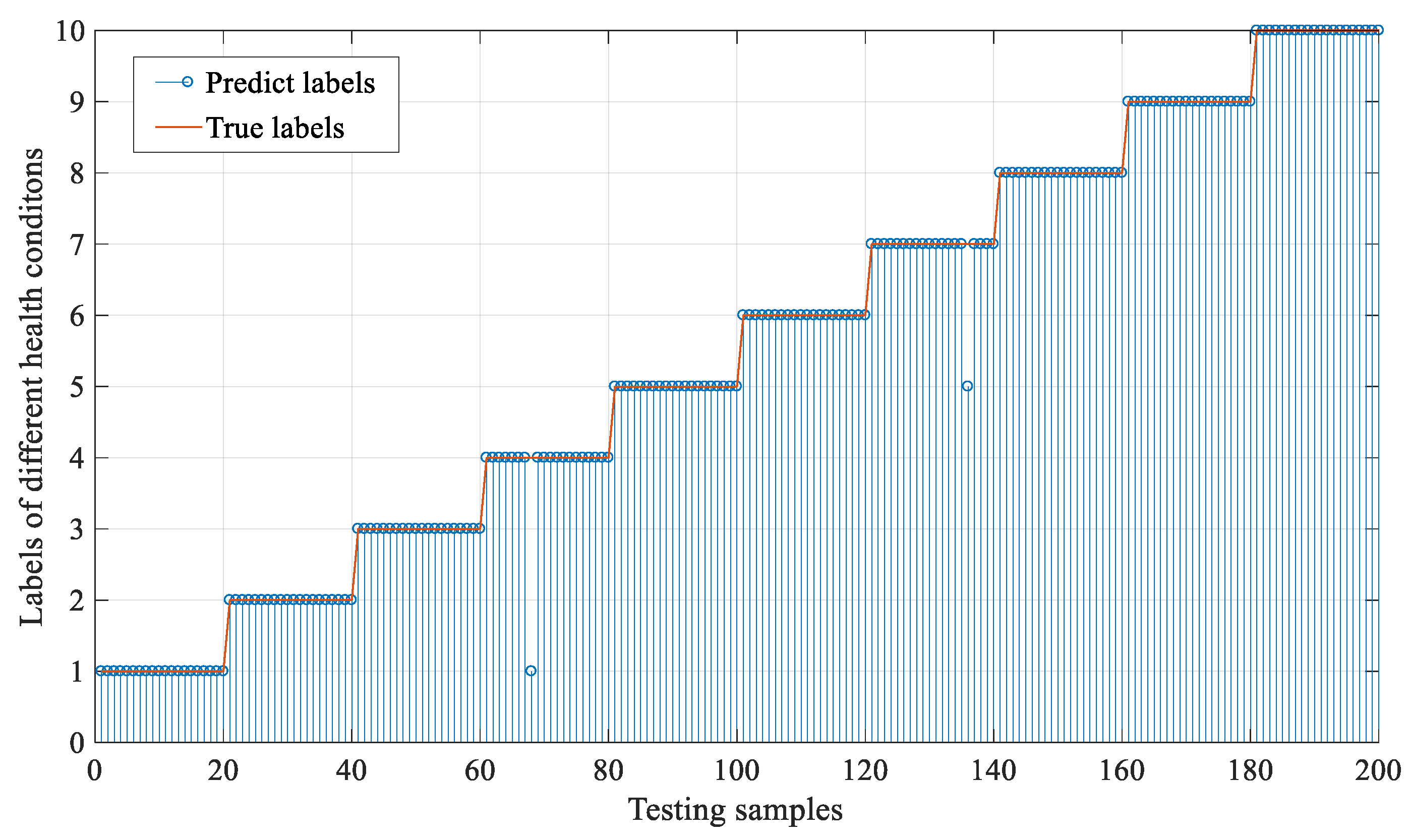
First, to present the diagnosis result of the proposed method, the real health condition labels and the predicted labels of the testing samples are shown in Figure 5. Generally, we can see that 99% of the testing samples are classified correctly, and only two of the listed testing samples are misclassified. In detail, only one sample of IF12 is misclassified as NO, and one sample of OF12 is misclassified as OF02. This could validate the effectiveness of the proposed method in classifying machine health conditions.
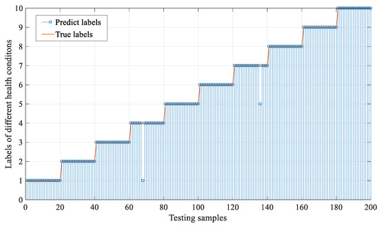
Figure 5.
The performance of the proposed method in diagnose testing samples.
Meanwhile, the convergence of the EKNN is also analyzed here to better demonstrate whether the proposed method can always converge well. The objective function values of the reconstruction process in the proposed method are shown in Figure 6. It can be seen that the optimization examples all converge when the iteration number reaches 150, and will not fluctuate with the optimization. In detail, their function values will shrink quickly with optimization iterations, but it will not reach zero values as the optimized value of objective function is not zero. In brief, the optimization process in Figure 6 confirms that the designed EKNN can be optimized and actually converge in experiments.
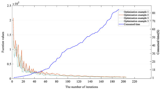
Figure 6.
The loss variation trend with the number of iterations.
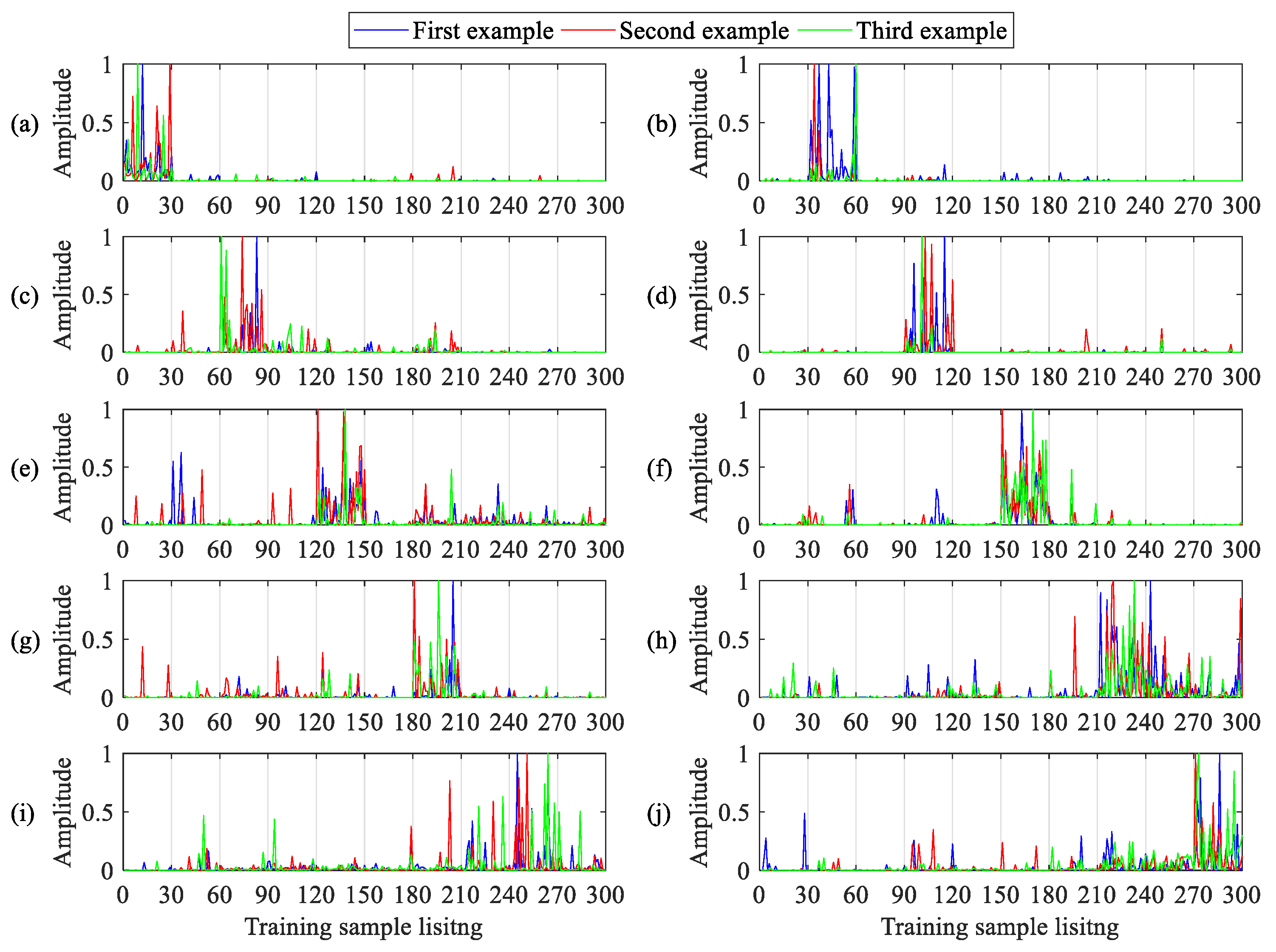
To show the correlation vectors obtained in the reconstruction process of EKNN, they are also shown in the sub-figures of Figure 7, respectively. Here, the number of training samples from each health condition used in the reconstruction process is 30, so there are totally 300 training samples here, which can be seen in the X-axis of each sub-figure. There are three samples from each corresponding health condition in each sub-figure, respectively. Meanwhile, each sub-figure has three samples, and samples of different health conditions are listed sequentially in the order shown Section 4.1.

Figure 7.
Correlation vectors between the target sample and the training samples. (a): NO, (b): IF02, (c): IF06, (d): IF12, (e): OF02, (f): OF06, (g): OF12, (h): BF02, (i): BF06, (j): BF12
Theoretically, the testing sample will have much higher correlations with the training samples from the same health condition, and the training samples with higher correlations are the nearest neighbors of the testing samples. For Figure 7a, it can be observed that the correlation vectors of the three testing samples from NO are active in training samples 1 to 30, which are the locations of NO. For other sub-figures, the situation is similar; all the correlation vectors of testing samples can obtain much higher correlations in their corresponding training samples. Generally, the situation presents that the proposed method can locate the nearest neighbors of each testing sample automatically in the reconstruction process via the obtained correlation vector, which verifies the effectiveness of the proposed method further.
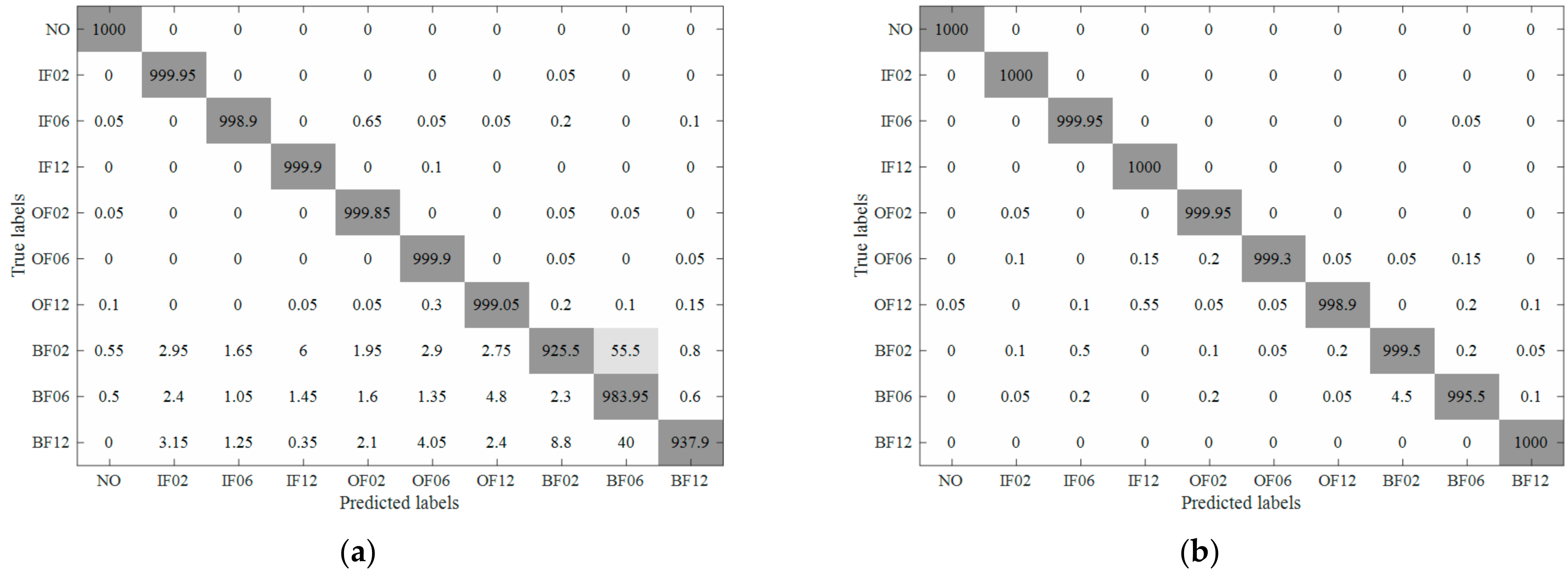
The averaged confusion matrices of KNN and EKNN are illustrated in Figure 8. Generally, samples of BF02 are most likely to be misclassified, and they are always misclassified as BF06, which is mainly because they are only distinct from each other in fault severity and have similar signals. For samples belonging to NO, they are diagnosed accurately because they have no faults and are highly distinct from all others.
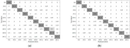
Figure 8.
The confusion matrices using original k-nearest neighbor (KNN) method and the proposed method: (a) the results of KNN and (b) the result of enhanced k-nearest neighbor (EKNN).
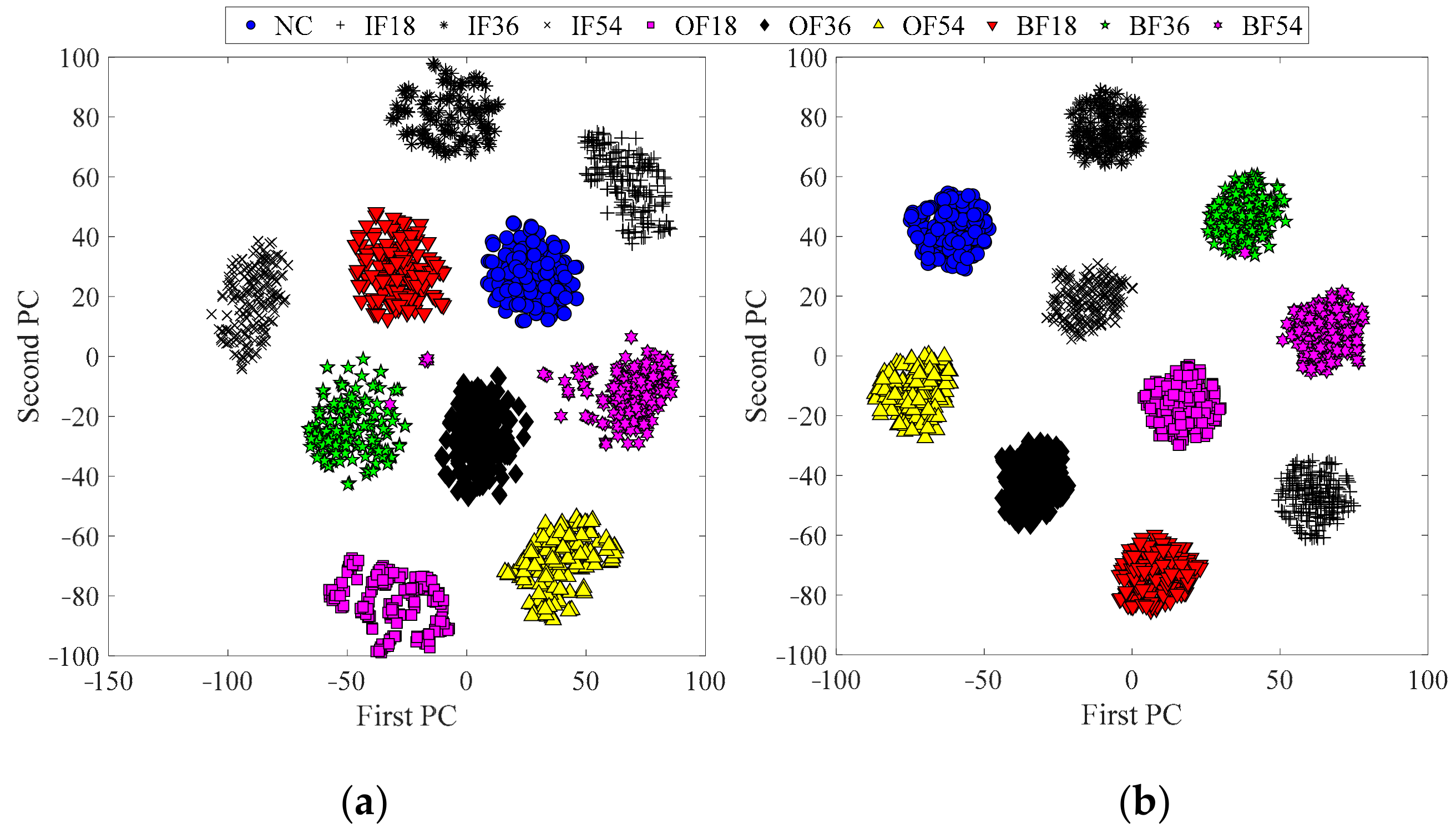
For clear feature presentation, the extracted feature vectors of samples are transformed into two-dimension ones via t-distributed stochastic neighbor embedding (t-SNE) [38], as shown in Figure 9. In detail, Figure 9a is the result obtained from raw samples; Figure 9b is the feature clustering result from SF. For convenience, health condition “NO” in the source dataset is denoted as “1”, and the others are denoted similarly using the listing order in Section 4.1. Generally, this presents that most of the features belonging to each class can be separated from those belonging to other classes in Figure 9a,b, and Figure 9b can gather the features from the same health condition more closely, which confirms that SF can extract highly discriminative features from inputs.
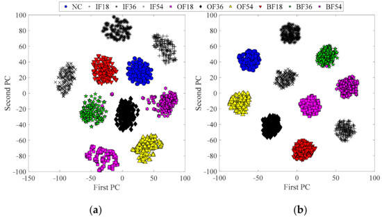
Figure 9.
Scatter plots of Principal Components (PCs) for the features learned in the bearing dataset: (a) features learned from raw samples; (b) features learned from SF.
To show the better performance of EKNN, we also calculated the precision and recall of the result. We can first obtain True Positive (TP), False Positive (FP), False Negative (FN) and True Negative (TN). Then, precision and recall can be calculated via
Precision = TP/(TP + FP)
Recall = TP/(TP + FN)
The results using KNN and EKNN are listed in Table 1 and Table 2, respectively, where the number of samples for each class is 200, and they are the overall results of 5 tries. As shown in Table 1 and Table 2, it is very clear that the performance using EKNN outperforms that using KNN almost in all classes. It can also be observed that EKNN can prevent misclassification more effectively than KNN, namely, FP and FP values of EKNN are much smaller than those of KNN.

Table 1.
The diagnosis result of KNN.

Table 2.
The diagnosis result of EKNN.
We also compared the executing time between EKNN and traditional KNN. As they are all training-free classification methods, we can obtain the executing time using only one sample. We denoted KNN using Euclid distance as KNN1 and denoted KNN using Euclid distance and Cosine distance as KNN2. Two distance evaluation matrices in KNN2 were combined with identical weight. The executing times of EKNN, KNN2 and KNN1 when classifying 200 were around 20, 15 and 10 s, respectively. Therefore, for each sample, EKNN, KNN2 and KNN1 need 0.1, 0.075 and 0.05 s, respectively. Although the executing time of EKNN is a little longer than that of KNN, the time cost is very beneficial due to the better performance of EKNN. On the other hand, the time length of the sample is 0.156 s, which is longer than the executing time using EKNN. Therefore, EKNN can also satisfy the requirement of online fault diagnosis, which benefits future online fault diagnosis well.
5. Conclusions
For fault diagnosis of rotating machineries, EKNN is proposed to diagnose faults in a more automatic way, which conducts feature extraction via unsupervised methods, and a new case-based classification method is proposed to diagnose faults via nearest neighbors determined automatically. Aiming to address the problems of the expensive and inefficient global search for nearest neighbors in KNN, the new classification method can perform a more efficient search via obtained correlation vectors of testing sample reconstruction. Particularly, as the feature extraction part is unsupervised and focuses on sparse feature extraction, the extracted features will be more discriminative for fault diagnosis. Meanwhile, unlabeled data can be used to train the feature extraction part simply, and a very small number of labeled samples is needed in its classification, which also needs no supervision and distinguishes it from other intelligent fault diagnosis methods.
Compared with existing case-based methods, it takes advantage of powerful feature extraction and realizes more automatic and precise classification. Compared with existing parameter-based diagnosis methods, it can utilize training samples and needs no training in classification. Meanwhile, when a new fault appears, the proposed method can utilize the case-based fault diagnosis part and learn to diagnose new faults, which is superior to existing parameter-based methods.
Extensive experiments conducted on a bearing fault dataset confirm the effectiveness of the proposed method. In addition, although the proposed method can take advantage of case-based methods, it still needs to investigate how to absorb new samples into the network to improve its self-learning process in our future work.
Author Contributions
Conceptualization, J.L. and W.Q.; methodology, J.L. and S.L.; software, W.Q. and R.C.; validation, J.L., W.Q. and S.L.; formal analysis, J.L., W.Q., and S.L.; investigation, S.L.; resources, S.L.; data curation, S.L.; writing—original draft preparation, W.Q.; writing—review and editing, J.L. and R.C.; visualization, J.L. and W.Q.; supervision, S.L.; project administration, S.L.; funding acquisition, J.L. and S.L. All authors have read and agreed to the published version of the manuscript.
Funding
This research was funded by the National Natural Science Foundation of China (51975276), the Major National Science and Technology Projects (2017-IV-0008-0045), the Advance Research Field Fund Project of China (61400040304), the National Key Research and Development Program of China (2020YFB1709801) and the Fundamental Research Funds for the Central Universities (1002-YAH20008).
Acknowledgments
The authors would like to thank Yingxian Zhang from China University of Geosciences for providing language help.
Conflicts of Interest
The authors declare no conflict of interest.
References
- Jiang, X.; Li, S.; Wang, Y. Study on nature of crossover phenomenon with application to gearbox fault diagnosis. Mech. Syst. Signal Process. 2017, 83, 272–295. [Google Scholar] [CrossRef]
- Guo, S.; Yang, T.; Gao, W.; Zhang, C. A novel fault diagnosis method for rotating machinery based on a convolutional neural network. Sensors 2018, 18, 1429. [Google Scholar] [CrossRef] [PubMed]
- Liu, J.; Tang, C.; Shao, Y. An innovative dynamic model for vibration analysis of a flexible roller bearing. Mech. Mach. Theory 2019, 135, 27–39. [Google Scholar] [CrossRef]
- Wang, Z.; Zhou, J.; Wang, J.; Du, W.; Wang, J.; Han, X.; He, G. A Novel Fault Diagnosis Method of Gearbox Based on Maximum Kurtosis Spectral Entropy Deconvolution. IEEE Access 2019, 7, 29520–29532. [Google Scholar] [CrossRef]
- Huang, W.; Gao, G.; Li, N.; Jiang, X.; Zhu, Z. Time-Frequency Squeezing and Generalized Demodulation Combined for Variable Speed Bearing Fault Diagnosis. IEEE Trans. Instrum. Meas. 2019, 68, 2819–2829. [Google Scholar] [CrossRef]
- Shen, C.; Wang, D.; Kong, F.; Tse, P.W. Fault diagnosis of rotating machinery based on the statistical parameters of wavelet packet paving and a generic support vector regressive classifier. Measurement 2013, 46, 1551–1564. [Google Scholar] [CrossRef]
- Han, T.; Liu, C.; Yang, W.; Jiang, D. Learning transferable features in deep convolutional neural networks for diagnosing unseen machine conditions. ISA Trans. 2019, 93, 341–353. [Google Scholar] [CrossRef]
- Liu, J.; Hu, Y.; Wang, Y.; Wu, B.; Fan, J.; Hu, Z. An integrated multi-sensor fusion-based deep feature learning approach for rotating machinery diagnosis. Meas. Sci. Technol. 2018, 29, 055103. [Google Scholar] [CrossRef]
- Yang, B.; Lei, Y.; Jia, F.; Xing, S. An intelligent fault diagnosis approach based on transfer learning from laboratory bearings to locomotive bearings. Mech. Syst. Signal Process. 2019, 122, 692–706. [Google Scholar] [CrossRef]
- Lei, Y.; Jia, F.; Lin, J.; Xing, S.; Ding, S.X. An Intelligent Fault Diagnosis Method Using Unsupervised Feature Learning Towards Mechanical Big Data. IEEE Trans. Ind. Electron. 2016, 63, 3137–3147. [Google Scholar] [CrossRef]
- Ngiam, J.; Chen, Z.; Bhaskar, S.A.; Koh, P.W.; Ng, A.Y. Sparse Filtering. In Proceedings of the 24th International Conference on Neural Information Processing Systems (NIPS), Granada, Spain, 12–17 December 2011; pp. 1125–1133. [Google Scholar]
- Qian, W.; Li, S.; Wang, J.; Wu, Q. A novel supervised sparse feature extraction method and its application on rotating machine fault diagnosis. Neurocomputing 2018, 320, 129–140. [Google Scholar] [CrossRef]
- Qian, W.; Li, S.; Jiang, X. Deep transfer network for rotating machine fault analysis. Pattern Recognit. 2019, 96, 106993. [Google Scholar] [CrossRef]
- Wen, L.; Li, X.; Gao, L.; Zhang, Y. A New Convolutional Neural Network-Based Data-Driven Fault Diagnosis Method. IEEE Trans. Ind. Electron. 2018, 65, 5990–5998. [Google Scholar] [CrossRef]
- Jia, F.; Lei, Y.; Guo, L.; Lin, J.; Xing, S. A neural network constructed by deep learning technique and its application to intelligent fault diagnosis of machines. Neurocomputing 2018, 272, 619–628. [Google Scholar] [CrossRef]
- Liu, R.; Meng, G.; Yang, B.; Sun, C.; Chen, X. Dislocated Time Series Convolutional Neural Architecture: An Intelligent Fault Diagnosis Approach for Electric Machine. IEEE Trans. Ind. Inform. 2017, 13, 1310–1320. [Google Scholar] [CrossRef]
- Shao, H.; Junsheng, C.; Hongkai, J.; Yu, Y.; Zhantao, W. Enhanced deep gated recurrent unit and complex wavelet packet energy moment entropy for early fault prognosis of bearing. Knowl. Based Syst. 2019, 188, 105022. [Google Scholar] [CrossRef]
- Miao, Q.; Zhang, X.; Liu, Z.; Zhang, H. Condition multi-classification and evaluation of system degradation process using an improved support vector machine. Microelectron. Reliab. 2017, 75, 223–232. [Google Scholar] [CrossRef]
- Qian, W.; Li, S.; Yi, P.; Zhang, K. A novel transfer learning method for robust fault diagnosis of rotating machines under variable working conditions. Measurement 2019, 138, 514–525. [Google Scholar] [CrossRef]
- Zhao, R.; Yan, R.; Chen, Z.; Mao, K.; Wang, P.; Gao, R.X. Deep Learning and Its Applications to Machine Health Monitoring: A Survey. arXiv 2016, arXiv:1612.07640. [Google Scholar] [CrossRef]
- Berredjem, T.; Benidir, M. Bearing faults diagnosis using fuzzy expert system relying on an Improved Range Overlaps and Similarity method. Expert Syst. Appl. 2018, 108, 134–142. [Google Scholar] [CrossRef]
- Yuan, K.; Deng, Y. Conflict evidence management in fault diagnosis. Int. J. Mach. Learn. Cybern. 2017, 10, 1–10. [Google Scholar] [CrossRef]
- Shi, P.; Yuan, D.; Han, D.; Zhang, Y.; Fu, R. Stochastic resonance in a time-delayed feedback tristable system and its application in fault diagnosis. J. Sound Vib. 2018, 424, 1–14. [Google Scholar] [CrossRef]
- Imani, M.B.; Heydarzadeh, M.; Khan, L.; Nourani, M. A Scalable Spark-Based Fault Diagnosis Platform for Gearbox Fault Diagnosis in Wind Farms. In Proceedings of the Information Reuse and Integration Conference, San Diego, CA, USA, 4–6 August 2017; IEEE: Piscataway, NJ, USA, 2017. [Google Scholar]
- Mohapatra, S.; Khilar, P.M.; Swain, R.R. Fault diagnosis in wireless sensor network using clonal selection principle and probabilistic neural network approach. Int. J. Commun. Syst. 2019, 32, e4138. [Google Scholar] [CrossRef]
- Wang, Q.; Liu, Y.B.; He, X.; Liu, S.Y.; Liu, J.H. Fault Diagnosis of Bearing Based on KPCA and KNN Method. Adv. Mater. Res. 2014, 986, 1491–1496. [Google Scholar] [CrossRef]
- Jiang, X.; Li, S. A dual path optimization ridge estimation method for condition monitoring of planetary gearbox under varying-speed operation. Measurement 2016, 94, 630–644. [Google Scholar] [CrossRef]
- Qian, W.; Li, S.; Wang, J.; An, Z.; Jiang, X. An intelligent fault diagnosis framework for raw vibration signals: Adaptive overlapping convolutional neural network. Meas. Sci. Technol. 2018, 29, 095009. [Google Scholar] [CrossRef]
- Gorunescu, F.; Belciug, S. Intelligent Decision Support Systems in Automated Medical Diagnosis. In Advances in Biomedical Informatics; Holmes, D., Jain, L., Eds.; Springer: Cham, Switzerland, 2018; Volume 137, pp. 161–186. [Google Scholar]
- Du, W.; Zhou, W. An Intelligent Fault Diagnosis Architecture for Electrical Fused Magnesia Furnace Using Sound Spectrum Submanifold Analysis. IEEE Trans. Instrum. Meas. 2018, 67, 2014–2023. [Google Scholar] [CrossRef]
- Melin, P.; Prado-Arechiga, G. New Hybrid Intelligent Systems for Diagnosis and Risk Evaluation of Arterial Hypertension. In Springer Briefs in Applied Sciences and Technology; Springer: Berlin/Heidelberg, Germany, 2018. [Google Scholar]
- Guo, G.; Wang, H.; Bell, D.A.; Bi, Y.; Greer, K. KNN Model-Based Approach in Classification. In Lecture Notes in Computer Science; Springer: Berlin/Heidelberg, Germany, 2003. [Google Scholar]
- Lei, Y.; Zuo, M.J. Gear crack level identification based on weighted K nearest neighbor classification algorithm. Mech. Syst. Signal Process. 2009, 23, 1535–1547. [Google Scholar] [CrossRef]
- Zhang, M.-L.; Zhou, Z.-H. ML-KNN: A lazy learning approach to multi-label learning. Pattern Recognit. 2007, 40, 2038–2048. [Google Scholar] [CrossRef]
- Chen, J.; Fang, H.; Saad, Y. Fast Approximate kNN Graph Construction for High Dimensional Data via Recursive Lanczos Bisection. J. Mach. Learn. Res. 2009, 10, 1989–2012. [Google Scholar]
- Luo, W.; Liu, W.; Gao, S. A Revisit of Sparse Coding Based Anomaly Detection in Stacked RNN Framework. In Proceedings of the 2017 IEEE International Conference on Computer Vision, Venice, Italy, 22–29 October 2017; IEEE: Piscataway, NJ, USA, 2017; Volume 1, pp. 341–349. [Google Scholar]
- Vlcek, J.; Lukšan, L. Generalizations of the limited-memory BFGS method based on the quasi-product form of update. J. Comput. Appl. Math. 2013, 241, 116–129. [Google Scholar] [CrossRef]
- Pezzotti, N.; Lelieveldt, B.P.F.; Van Der Maaten, L.; Höllt, T.; Eisemann, E.; Vilanova, A. Approximated and User Steerable tSNE for Progressive Visual Analytics. IEEE Trans. Vis. Comput. Graph. 2015, 23, 1739–1752. [Google Scholar] [CrossRef] [PubMed]
Publisher’s Note: MDPI stays neutral with regard to jurisdictional claims in published maps and institutional affiliations. |
© 2021 by the authors. Licensee MDPI, Basel, Switzerland. This article is an open access article distributed under the terms and conditions of the Creative Commons Attribution (CC BY) license (http://creativecommons.org/licenses/by/4.0/).

