Learning Knowledge Using Frequent Subgraph Mining from Ontology Graph Data

Abstract

In many areas, vast amounts of information are rapidly accumulating in the form of ontology-based knowledge graphs, and the use of information in these forms of knowledge graphs is becoming increasingly important. This study proposes a novel method for efficiently learning frequent subgraphs (i.e., knowledge) from ontology-based graph data. An ontology-based large-scale graph is decomposed into small unit subgraphs, which are used as the unit to calculate the frequency of the subgraph. The frequent subgraphs are extracted through candidate generation and chunking processes. To verify the usefulness of the extracted frequent subgraphs, the methodology was applied to movie rating prediction. Using the frequent subgraphs as user profiles, the graph similarity between the rating graph and new item graph was calculated to predict the rating. The MovieLens dataset was used for the experiment, and a comparison showed that the proposed method outperformed other widely used recommendation methods. This study is meaningful in that it proposed an efficient method for extracting frequent subgraphs while maintaining semantic information and considering scalability in large-scale graphs. Furthermore, the proposed method can provide results that include semantic information to serve as a logical basis for rating prediction or recommendation, which existing methods are unable to provide.

1. Introduction

Since the emergence of the concept of the Semantic Web, ontologies used in information science have been constructed by various agents across diverse domains to store and organize information. Ontology is a semantic data model that specifies concepts and the relationships between the concepts [1]. An ontology that defines the “type” of “things” and reveals the semantic relationship between the “things” is itself an enormous graph and a collection of various types of information.

Specifically, experts in each field define a domain ontology to represent their knowledge about classes, properties, and instances in their point of view, according to W3C’s Web standards such as Resource Description Framework (RDF) and Web Ontology Language (OWL). In this paper, we referred to terminological component (TBox) as ‘ontology’ or ‘schema’ and assertion component (ABox) as ‘instance graph’ or ‘knowledge graph’. In other words, a database that stores instance-level data using the graph structure of ontology (class/property relations) is a knowledge graph. We refer to such a knowledge graph as “ontology graph data” or “ontology-based knowledge graph” in our study.

If a frequent pattern (i.e., frequent subgraph) is discovered in an ontology-based knowledge graph, then the semantic information it contains can be utilized to expand the schema of that domain or acquire new application insights. For example, if it is discovered that certain instances in a knowledge graph possess common attributes, they can be grouped together and defined as a new class, thus expanding knowledge.

However, considering that ontology includes semantic information, it is impossible to apply a frequent subgraph mining algorithm to general graphs that simply consist of nodes and edges. Moreover, as the data consist of one large graph rather than a set of graphs, the occurrence must be divided into measurable units to calculate the frequency, and dividing by item set (transaction) as in previous methods results in loss of graph information.

Accordingly, this study proposed a methodology to effectively extract frequent subgraphs while retaining the graph information. First, this study presented a novel method of decomposing a large-scale instance graph built based on an ontology into small unit subgraphs. The unit subgraphs serve as the unit of occurrence to calculate the frequency and support, and instance triples with support beyond the threshold are regarded as candidates for chunking. The candidate instance triple becomes a new chunk, and candidate generation and chunking are repeated to extract the frequent subgraph.

The usefulness of the information contained in these extracted frequent subgraphs was verified through experiments. Using a movie ontology containing information on the actors, genre, and director of a movie, a new ontology in which user rating is linked was created, and the frequent subgraphs were extracted from the instance graph constructed based on the new ontology. The frequent subgraphs and new item graphs were compared to predict the rating, and the accuracy of the recommendation to the user was evaluated against other recommendation algorithms. The results confirmed that the proposed methodology outperforms the other algorithms in terms of accuracy and F1-score, demonstrating that the methodology proposed in this study is useful for real applications.

1.1. Related Works

1.1.1. General Frequent Subgraph Mining

Frequent subgraph mining (FSM), a field of graph mining, relates to the investigation of methods to find patterns that frequently occur (i.e., occur more than the threshold) in a graph dataset [2]. Typically, FSM algorithms identify a suitable starting node from the graph, apply the depth-first search (DFS) or breadth-first search (BFS) strategy to create candidate subgraphs, and then count the frequency of each candidate to extract the patterns.

The most frequently cited FSM algorithm is gSpan [3], which supports undirected graphs, uses DFS, and employs the minimum DFS code to specify the subgraphs uniquely. Several other FSM algorithms have been developed for biochemical graph data. MoFa [4] attempted to extract the patterns from graphs representing molecules. FFSM [5] attempted to find subgraphs from protein structures with a small number of labels but large and dense characteristics. Nijssen and Kok proposed an integrated algorithm called GASTON to find frequent paths, trees, and graphs [6]. These studies primarily focused on graph representation methods, methods for quickly and effectively generating candidates, and the isomorphism test, which confirms whether subgraphs belonging to different graphs are homogeneous (which is necessary for counting the frequency).

1.1.2. Frequent Subgraph Mining on Knowledge Graph

Subgraph mining with an ontology-based knowledge graph differs from general subgraph mining. General FSM algorithms primarily address the structure of the final extracted frequent subgraphs; that is, the fact that the specific structure frequently occurs in the dataset is important. However, if FSM is applied to an ontology-based knowledge graph, then the identified frequent subgraphs will have interpretable meanings, and these ‘meanings’ can be of use according to the ontology domain. For example, it is possible to explain that a user likes action movies starring Tom Cruise because a frequent subgraph from his data has a triple <Tom Cruise, Acting, Movie> with <Movie, MovieGenre, action>. That is, one can get information for interpretation of the results (frequent subgraphs) from an ontology-based knowledge graph.

In a large-scale knowledge graph, it is necessary to determine a suitable unit or transaction for counting the occurrences to find the frequent subgraphs. Accordingly, to perform frequent subgraph mining, numerous studies converted the graph structure into a set of transactions comprising a series of items and then solved it as a problem of association rule mining or frequent pattern mining [7,8,9,10,11]. These methodologies have the disadvantage that the semantic information of the graph is lost in the process of creating the transactions. Moreover, it is difficult to regard the extraction results as frequent subgraphs, even though it was approached through association rule mining (frequent pattern mining).

On the other hand, if we look at recent studies related to knowledge graph, Wang et al. predicted human mobility activity embedding spatial knowledge graph [12], Zhou et al. presented conversational recommendation approach via KG based semantic fusion [13], and Li et al. extracted triplet samples from the knowledge graph [14]. We confirm that many studies, including those not mentioned here, are proceeding with neural network (such as graph recurrent neural network, deep neural network, graph convolutional neural network) based research. While these studies are focused on the performance of solving target problems, our research aims to have explanatory power solving problems at a reasonable level.

1.1.3. Recommendation Algorithm

Research on recommendation using a knowledge graph has recently drawn much attention. Palumbo et al. presented entity2rec, a recommender system based on property-specific knowledge graph embeddings and introduced a new way of creating property-specific sub-graphs [15]. Using Linked Open Data (LOD) knowledge base such as “DBpedia”, Recommender System with LOD (RS-LOD) model for cold start issue and Matrix Factorization model with LOD (MF-LOD) for data sparsity problem was developed [16]. In a similar approach, Wang et al. proposed a new semantic similarity measure based on semantic information in the LOD knowledge base, which is a hybrid measure based on feature and distance metrics [17].

As the study focused on selection and embedding of semantic features, Noia et al. showed how ontology-based (linked) data summarization can drive the selection of properties/features useful to a recommender system [18]. Anelli et al. showed how to initialize latent factors in Factorization Machines by using semantic features coming from a knowledge graph in order to train an interpretable model [19]. These studies did not directly focus on knowledge expansion or recommendation algorithms fully utilizing knowledge graphs, and knowledge graphs were used as a source of additional information or only some features.

The objective of our study is not to develop a recommender system but to apply the proposed methodology to a recommendation application for performance evaluation. This evaluation is needed to verify whether the frequent subgraphs extracted in our experiment adequately reflect the meaning of the original graph. Accordingly, we describe several collaborative filtering algorithms used in the experiment.

Four algorithms were used for comparison. First, the kNN (k Nearest Neighborhood) inspired algorithm utilizes information from neighbors close to the user to recommend items [20]. The other three algorithms are matrix factorization algorithms, which decompose the user-item matrix into two matrices [16]. We used the Singular Value Decomposition (SVD) [21], SVD++ [20], and Non-negative Matrix Factorization (NMF) [22] algorithms for the comparison.

As kNN, SVD, SVD++ and NMF algorithms were not developed for ontology graph data, the calculations were performed based on numerical data, and the recommendations were made without knowing the semantic information contained in ontology graph data. Hence, it is difficult to logically explain why certain items are recommended. The proposed methodology not only outperforms these algorithms, but also explains why the items were recommended. Such merits raise the possibility that our approach can be developed into an algorithm for collaborative filtering.

2. Methodology

This section describes a novel and efficient methodology for finding frequent subgraphs in large-scale graphs and applies it to an actual case of rating prediction to verify the superior performance and applicability of the proposed methodology.

2.1. Frequent Subgraph Mining

As mentioned above, the existing methodologies for frequent subgraph mining primarily focused on enhancing computational performance without considering the semantic information for each node and edge, mainly from the perspective of candidate generation or the isomorphism test. The proposed methodology assumes an ontology graph and utilizes semantic and mining query information to decompose a large graph into small unit subgraphs, thereby maintaining semantic information and improving computational efficiency.

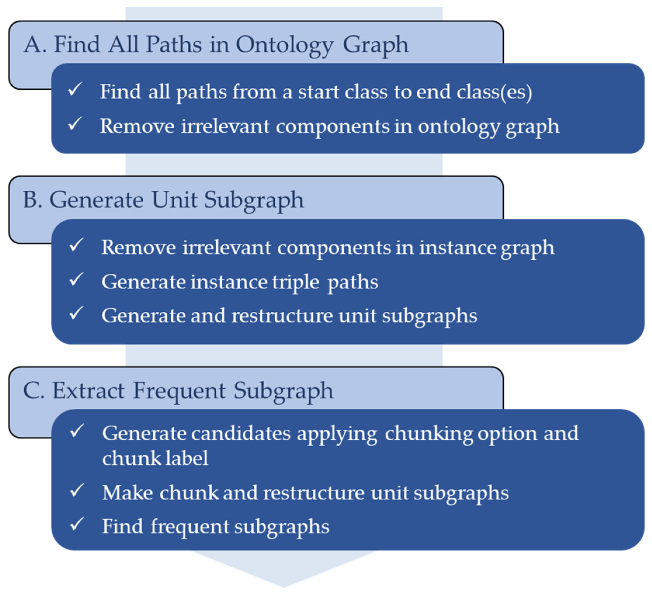
As shown in Figure 1, the methodology comprises three main steps. The first is a preprocessing step in which the mining query is used to find all possible paths in the ontology graph while removing irrelevant components. In the second step, the irrelevant components are removed from the instance graph, after which instance triple paths corresponding to the paths of the ontology graph obtained in the first step are generated, through which the unit subgraphs are generated and restructured. In the third and final step, using these generated unit subgraphs as the unit of frequency, chunking and candidate generation considering the chunk option and chunk label are repeated until the threshold is satisfied, after which the final frequent subgraphs are extracted.

Before explaining the detailed methodology, several terms are defined, and their meanings and assumptions used in this study are described. The ontology graph is shown in Figure 2a. Each class (node) and property (edge) are unique in a total ontology graph and multiple properties (multi edge) are allowed. Figure 2b is an example of an instance graph. A class of ontology graphs has one or more instances, and one or more properties between classes are inherited by the property between two instances.

Owing to the enormous cost of directly searching for frequent subgraph patterns in an entire graph, this study attempts to improve the efficiency of this process by dividing the entire graph into “unit subgraph.” “Unit subgraph” is a set of instances and properties generated by the mining query. It comprises all paths from an instance of a start class to all instances of the end classes and becomes the basic unit for calculating the frequency.

“Mining Query” is basically a concept for defining the extent of the subgraph when dividing a large graph into subgraphs of small units. In this study, knowledge graphs based on the ontology graph are the subject of the study, so we tried to make the most use of the information that ontology has. When an expert with information about a specific domain ontology performs frequent subgraph mining on his ontology-based knowledge graph, “Mining Query” allows his domain knowledge to be fully reflected in the analysis.

The “Mining Query” concept is defined as follows.

Mining Query: = (SC, EC, CO)

(1)

The mining query comprises three parts, which are defined as follows:

• SC (Start Class): the start class of an ontology graph; each instance of this class is a start node of a unit subgraph;
• EC (End Class): a set of end classes; all instances of these classes are end nodes of the unit subgraph;
• CO (Chunking Option): chunking option; a set of classes to be chunked considering instances as their classes in a unit subgraph (if not specified, instance level chunking is performed).

For example, given a mining query “Q” (Equation (2)) has the following meanings: “We try to find the frequent pattern in the linked relationship of “User” and “Academy”, “Genre” and “Rating” and in the case of “WatchingEvent” and “Movie” classes, the information in their instances is not used for analysis.” This approach is significant in that it can incorporate domain information of experts into the frequent subgraph mining.

Q = (User, {Academy Genre Rating}, {WatchingEvent Movie})

(2)

In the example of Equation (2), the start class for composing the unit subgraphs becomes the “User” class, the three classes of “{Academy Genre Rating}” are used as the end classes, and during candidate generation, the instances of “{WatchingEvent Movie}” classes are considered as a single class called “WatchingEvent” and “Movie”, respectively.

2.1.1. Ontology Graph Processing

Figure 3 shows an example of a general ontology graph, which considers the mining query in Equation (2).

The ontology resources in the sentence “Tenet is directed by Christopher Nolan” are represented by class and property in the ontology graph. The ovals “(1)Movie” and “(2)Person” in Figure 3 become classes representing the instances “Tenet” and “Christopher Nolan,” respectively, and the rectangle on the edge connecting them, “[4]DirectedBy”, acts as a property. Reflecting the mining query in Equation (2), the sky blue oval (“(4)User”) in Figure 3 becomes the start class, the yellow ovals (“(7)Academy”, “(6)Genre”, “(3)Rating”) become the end classes, and the ovals “(0)WatchingEvent” and “(1)Movie” are regarded only as classes without considering the differences in the instances belonging to them in candidate generation. In addition, to maintain the generality of the ontology, this study considers the reflexive property “[1]AssociatedWith” displayed in green and the multiple properties between the “(1)Movie” and “(2)Person” classes displayed in orange (“[2]Acting”) and black (“[4]DirectedBy”) lines, through which paths are found in the ontology graph and instance triple paths are found in the instance graph.

The ontology graph in Figure 3 is represented in the form of the data structure in

Table 1. Ontology graph data structure.

Class	Property	Class
(0)Watching Event	[0]WatchedMovie	(1)Movie
(1)Movie	[1]AssociatedWith	(1)Movie
(2)Person	[2]Acting	(1)Movie
(3)Rating	[3]RatingEvent	(0)WatchingEvent
(1)Movie	[4]DirectedBy	(2)Person
(4)User	[5]UserWatched	(0)WatchingEvent
(1)Movie	[6]MadeBy	(5)Company
(1)Movie	[7]ClassifiedBy	(6)Genre
(2)Person	[8]EducatedFrom	(7)Academy

in an actual application.

Next, based on the data expressed in the above form, a matrix with rows and columns as classes is generated, which is used to find all paths from the start class to the end class (Figure 4). We assume that a path contains no repeated properties.

In Figure 4, the reflexive property mentioned above is reflected in the paths in the form of “[1]AssociatedWith” between “(1)Movie” and “(1)Movie” classes, and the multiple properties are shown as two property paths, where the order of “[2]Acting” and “[4]DirectedBy” is changed.

Finally, Figure 5 shows the clean ontology graph after removing the components that do not belong to the paths between the start class and end class, that is, the components unrelated to the given mining query.

2.1.2. Unit Subgraph Generation

In this step, using this clean ontology graph and paths, the irrelevant components are removed from the instance graph. The instance triple paths are obtained, and then the unit subgraphs are generated and restructured. Figure 6 and

Table 2. Instance graph data structure.

ID	Class	Instance ID	Instance	Property	Class	Instance ID	Instance
1	Watching Event	W101	U1_M01	Watched Media	Movie	M01	Movie_01
5	Person	P01	Person_01	Acting	Movie	M01	Movie_01
13	Movie	M02	Movie_02	Associated With	Movie	M02	Movie_02
16	Movie	M01	Movie_01	Directed By	Person	P01	Person_01

show an example of an initial instance graph and some of its data structures.

As shown in the instance graph data structure of Table 2, the reflexive property and the multiple properties mentioned above were properly reflected in IDs 13, 5, and 16. Figure 7 shows the instance graph after removing the instance components (ID 7) unrelated to the mining query, as in the ontology graph. However, unlike the reflexive property in the ontology graph, a reflexive property connecting the same instances is not allowed at the instance level; therefore, the corresponding triple instances (ID 13) are removed.

Figure 8 shows the instance triple paths obtained using the ontology graph and paths. The instances in the instance graph belong to a specific class. Because these classes are found in the paths and the properties of the instance graph also match the properties of the paths, it is not difficult to obtain the instance triple paths. In this example, the start class is “User” and the instances belonging to that class are User_1, User_2, and User_3. Hence, the set of instance triple paths that will compose the three unit subgraphs is obtained.

The unit subgraphs displayed in Figure 9 are generated by combining the instance triple paths obtained for each instance of the user class. The rectangles indicate where the instance triple ID of the original triple is changed to a new ID. This process is meant to maintain the graph structure of each unit subgraph in the chunking step performed later. These unit subgraphs then become the basic unit for calculating the frequency. The candidate generation and chunking processes in the next step are performed for each unit subgraph.

2.1.3. Frequent Subgraph Extraction

In this step, the chunking option and chunk label are first applied to the instance triples of the unit subgraphs. Then, the instance triples with support that satisfy the specified threshold are selected as the candidates and chunked, after which the labels for the chunks are applied to restructure the unit subgraphs. Figure 10 shows the process for which the chunking option is applied. The corresponding instances of the unit subgraph are considered as a class in the given chunking option “{Watching Event Movie}” in order to be calculated at the class level rather than the instance level. For the instance triple “<Movie_01, Directed By, Person_01>”, the “Movie_01” instance is changed to the label “Movie” and the frequency is calculated considering the instance triple “<Movie, Directed By, Person_01>.”

The definitions for the frequency and support used in this study are explained as follows.

Definition 1.

The support of a subgraph g is defined as

$$su{p}_G\left(g\right)=\frac{F}{T}$$

(3)

where F (Frequency) is the number of unit subgraphs in which the subgraph g occurs, and T is the number of unit subgraphs in a database $G=\left\{G_1,G_2, \cdots ,G_n\right\}$ consisting of a collection of unit subgraphs. F is calculated as one count per unit subgraph regardless of whether g occurs once or more than once in a unit subgraph.

The subgraphs in this study are composed of a set of instance triples and chunks, that is, sets of instance triples to be newly labeled. The threshold is a criterion for whether an instance triple or chunk can become a chunking candidate. In the case of Figure 11, because the threshold is assumed to be 0.5, the instance triples with a support value of 0.67 or 1.00 become the candidates.

Meanwhile, the instances corresponding to the “{Watching Event Movie}” classes are changed to class, as shown in green, and the frequency and support are calculated at the class level. Although this triple appears twice in the “User_3” unit subgraph, the frequency is incremented as one, as the number of unit subgraphs is counted.

As shown in Figure 11, the criteria to determine which of the four candidates that satisfy the threshold should actually be chunked were applied in the following order.

• Higher support,
• Lager size of chunk,
• Random if the preceding conditions are the same.

In Figure 12, the instance triple “<Watching Event, Watched Movie, Movie>” is targeted for chunking, and chunking is actually performed. The result is shown in the changed appearance of each unit subgraph and the ID and label newly attached to the new chunk (“Watching Event-Movie”). For example, in the unit subgraph of “User_1”, “_1:1” is the instance ID for managing the newly created chunk as a new instance, and “[_1:4]” signifies that the newly created chunk (new instance) in each unit subgraph is identical. This is the label used in the next candidate generation. Managing the chunk (new instance) in these two forms satisfies the goal of maintaining the unit subgraph’s graph structure regardless of chunking. That is, before chunking, instances such as “Watching Event” and “Movie” that comprised the chunk were connected with instances such as “Rating_40” and “Person_01”, respectively. After chunking, a new chunk (such as “_1:1”, “_1:15”, “_1:6”, and “_1:19”) is connected with instances such as “Rating_40” and “Person_01” by the same property.

Figure 13, Figure 14 and Figure 15 show the repetition of the process until there is no instance triple (or chunk) with support that satisfies the threshold. In this example, no candidate is generated after performing the fourth chunking. The squares to the right of each figure show how the chunk generated in the previous step grows in the next step. Accordingly, chunking ends in steps 2 or 3 in certain unit subgraphs and in step 4 in others.

Figure 16 shows the final frequent subgraphs found in the entire instance graph after performing all the processes. Three frequent subgraphs were found in this example; the frequent subgraph Ⓐ (subgraph in blue polygon in Figure 16) consists of four triples among the triples of the original instance graph. That is, “<R50, Rating Event, Watching Event>”, “<Watching Event, WatchedMovie, Movie>”, “<Movie, Directed By, P02>”, and “<P02, Educated From, AC02>” constitute the frequent subgraph Ⓐ found in this example.

Thus far, this chapter explained the process of addressing the difficulty of finding frequent patterns in a large-scale graph using an ontology graph, instance graph, and mining query for generating unit subgraphs. We decomposed the entire graph into unit subgraphs and calculated the frequency and support by the number of unit subgraphs according to the mining query. This method has not been reported yet. In fact, given that finding frequent subgraphs in a graph is known as an NP-hard problem, the methodology proposed in this study can serve as a highly effective alternative. The next subsection explains the application of the extracted frequent subgraph for movie rating prediction.

2.2. Movie Rating Prediction

2.2.1. User Rating Ontology and Rating Graph

The user rating ontology was defined to predict the ratings using the frequent subgraphs. In the user rating ontology, the purchase or consumption events of each user are combined with the basic domain ontology, which consists of items and item attributes. These events contain the degree of preference, that is, the rating information that the user assigns to the item. For example, Figure 17 below shows the user rating ontology schema for the movie domain. This is created by combining the user, watching event, and rating classes with the domain ontology that contains the information about the movie. The actual instance graph for this schema will connect one user to multiple movies.

We apply the algorithm in Section 2.1 to a given instance graph based on the User Rating Ontology. Among the extracted frequent subgraphs, one or more subgraphs related to the rating was defined as the Rating Graph; i.e., it is a set of rating subgraphs. In Figure 18a, the rating graph contains a pattern based on the rating evaluated by the user. This pattern is an attribute set that influences the user’s decision to assign a high or low rating to the item. Accordingly, this can be used to predict the degree of preference and rating for other items. On the basis of these predictions, movies that the user is likely to rate highly can be found and recommended.

2.2.2. Graph Similarity and Entropy

The rating graph is a set of patterns (i.e., instance triples), but it is also a graph. Accordingly, this study measures the graph similarity between the target item graph and the rating graph containing the knowledge experienced by the user, and the most similar rating is used as the predicted value. To calculate the graph similarity, a modified Levenshtein distance (edit distance) [23] was used, and entropy was defined for the cost of adding and deleting triples. Typical definition of Graph Edit distance (GED) is known as follows.

Definition 2.

Given a set of graph edit operations (also known as elementary graph operations), the graph edit distance ($GED\left(g_1,g_2\right)$) between two graphs $g_1$ and $g_2$ can be defined as

$$GED\left(g_1,g_2\right)=\underset{\left(e_1, \dots e_k\right)\in P\left(g_1,g_2\right)}{\min }{\displaystyle \sum }_{i=1}^{k}c\left(e_i\right)$$

(4)

where $P\left(g_1,g_2\right)$ is the set of edit paths transforming $g_1$ into $g_2$ and $c\left(e\right)\ge 0$ is the cost of each graph edit operation $e$. In this study, edit operations are addition and deletion of triple considering the graph as a set of triples and paths is not needed when considering characteristics of target graph consisting of “movie” and its attributes. In terms of the cost of operation, addition and deletion have the same value, but different values by triple. The concept of “entropy” is defined to work as a kind of cost.

Entropy was defined as the proportion of information contained in each triple or graph in all frequent subgraphs obtained in the previous step. Figure 18 shows the graphs for which the graph similarity must be measured. In this process, each triple constituting the rating graph represents frequency information indicating the number of times they occur in the training data. Each triple contains a different amount of information; therefore, the edit distance is calculated with different contributions corresponding to their different entropies rather than equal contributions.

Before describing the method for calculating the entropy, several definitions should be presented. First, the rating graphs consist of the subgraphs extracted for each rating, and the entropy is calculated considering the entire rating subgraph set. $m$ is the number of triples in the rating graph, and $n$ is the number of rating classes that the user has evaluated. In the case of the movie rating dataset used in the experiment of Section 3.1, the user can assign a rating from 0.5 to 5.0 in units of 0.5, in which case $n=10$.

Rating Graph Entropy (RGE) of rating $j$ is the proportion of each rating in the rating subgraph set. Accordingly, it is obtained by dividing the sum of the triple frequencies constituting each rating graph by the sum of all triple frequencies of all ratings.

$$RG{E}_j=\frac{{{\displaystyle \sum }}_{i=1}^m{f}_{ij}}{{{\displaystyle \sum }}_{j=1}^n{{\displaystyle \sum }}_{i=1}^m{f}_{ij}}$$

(5)

where $f_{ij}$ is the frequency of the triple $i$ in rating $j$. In each rating graph, the importance of the triple is assigned differently. The triple with the highest frequency in each rating graph is defined as the Seed Triple (colored section in

Table 3. Frequency and entropy of triple by rating.

Instance Triple			Rating 3.0		Rating 4.0
Subject	Property	Object	Freq.	Entropy (NTE)	Freq.	Entropy (NTE)
Movie	Sound	PERS_0015893	0	0.000	2	0.031
Movie	MovieGenre	GENR_00018	3	0.069	0	0.000
Movie	MoviePopularity	POPU_U100	12	0.278	0	0.000
Movie	MovieGenre	GENR_00028	2	0.046	0	0.000
Movie	Acting	PERS_0000518	2	0.046	0	0.000
Movie	MovieGenre	GENR_00014	2	0.046	0	0.000
Movie	MovieGenre	GENR_00035	4	0.093	2	0.031
Movie	MovieVote_Average	VOAV_U90	0	0.000	5	0.077
Movie	MovieVote_Average	VOAV_U80	4	0.093	0	0.000
Movie	MovieGenre	GENR_00012	2	0.046	3	0.046
Movie	MovieRevenue	REVE_U100	8	0.185	5	0.077
Movie	MovieGenre	GENR_10749	0	0.000	2	0.031
Movie	MovieVote_Count	VOCO_U100	8	0.185	6	0.092
Movie	MovieVote_Average	VOAV_U50	2	0.046	0	0.000
Movie	MovieGenre	GENR_00053	2	0.046	0	0.000
Movie	MovieCountry	COUN_US	26	0.601	26	0.399
Movie	MovieRuntime	RUNT_U90	2	0.046	0	0.000
Movie	MoviePopularity	POPU_U90	0	0.000	2	0.031
Movie	MovieGenre	GENR_10751	3	0.069	2	0.031
Movie	MovieBudget	BUDG_U80	2	0.046	0	0.000
Movie	Acting	PERS_0001100	2	0.046	0	0.000
Movie	Acting	PERS_0005344	0	0.000	2	0.031
Total triple frequency			102		65
RGE by rating				0.611		0.389
Total NTE				1.989		0.874
Number of triples in rating graph				17		11
ANTE by rating				0.117		0.079

Colored cells represent the seed triple of each rating subgraph.

), and the entropy of the seed triple has the same value as the RGE of the rating to which the seed triple belongs. The entropy of a triple that is not a seed triple is calculated by dividing the frequency of the triple by that of the seed triple. Thus, Triple Entropy (TE) is the ratio of the information indicating the influence or dominance of each triple in the rating graph. $s{f}_j$ is the frequency of the seed triple in rating $j$.

$$T{E}_{ij}=\frac{f_{ij}}{s{f}_j}$$

(6)

The Normalized Triple Entropy (NTE) of each triple is calculated as the product of TE (Equation (6)) and RGE (Equation (5)). This is the normalized entropy used when adding or deleting each triple. The entropy values in Table 3 are NTEs for each rating and instance triple calculated accordingly.

$$NT{E}_{ij}=T{E}_{ij}\times RG{E}_j$$

(7)

When a triple that is not in the rating subgraph set must be added, a value that serves as the edit distance cost is necessary. As shown in Equation (8) below, this Average Normalized Triple Entropy (ANTE) by rating is calculated by dividing the normalized entropy sum of the rating graph triples by the number of triples of the rating graph.

$$ANT{E}_j=\frac{{{\displaystyle \sum }}_{i=1}^{m}NT{E}_{ij}}{m}$$

(8)

The values of Equations (5), (7) and (8) can be calculated for each instance triple and rating, as shown in Table 3.

2.2.3. Rating Prediction

As shown in Figure 19, the cases encountered in rating prediction for each user can be categorized into three types. The first is the case of an intersection when comparing all triple sets of the entire rating subgraph set with the triple sets of the corresponding item graph, which is explained in detail in (A). The second is the case with no intersection, and the third is the case in which frequent subgraphs for each user are not extracted in the beginning. The method for handling both cases is the same and is explained in (B).

(A) Rating–Item Graph Similarity based Prediction

In this case, there is an intersection when comparing all triple sets of the entire rating subgraph set with the triple sets of the corresponding item graph, and the similarity of the item graph with the rating graph is calculated and compared to predict the rating.

First, the triples included in both the rating subgraph set and the item graph are selected. Next, to calculate the similarity between the item graph and rating graph, the Levenshtein distance (i.e., the cost of converting the rating graph to the item graph) is calculated using the previously obtained NTE and ANTE. The edit distance involves the costs of both deleting and adding a triple, and a smaller total cost indicates greater similarity. This study used a method in which the NTE is subtracted when deleting a triple in the rating graph, and the ANTE is subtracted when adding a triple not in the rating graph. The value obtained by multiplying the RGE by the number of intersections is used as the baseline value to subtract from, thereby considering the proportion of the rating graph and importance of the user preferred attribute. Finally, for a given target item graph, the rating of the rating graph with the highest similarity is predicted.

Table 4. Rating prediction result.

Target Instance	Rating 3.0	Rating 4.0	Actual	Predicted
MOVI_000408	4.011	1.888	3.0	3.0
MOVI_000581	3.894	3.967	4.0	4.0
MOVI_002164	4.011	1.888	3.0	3.0
MOVI_002636	1.894	0.888	3.0	3.0
MOVI_008984	2.894	0.808	3.0	3.0
MOVI_009255	2.011	0.967	3.0	3.0
MOVI_036593	−0.106	2.126	3.0	4.0

shows the final rating prediction result; in this example, only the rating subgraphs of ratings 3.0 and 4.0 are in the extracted frequent subgraph. For each movie, a higher similarity rating graph is shown in blue and "Actual" and "Predicted" columns are shown in beige if they are the same.

(B) Item–Item Graph Similarity Based Prediction

This method is applied when there is no intersection between the rating graph and item graph and when there is no extracted rating subgraph. In either case, the similarity between the rating graph and the item graph cannot be calculated.

The similarities between all item graphs (items in training set) and the target item graph were calculated, and the rating of the most similar item was predicted. As in (A), the Levenshtein distance is used; however, because entropy cannot be used in this case, the cost of adding and deleting the triple is the same.

If multiple items have the same similarity, then to break the tie, the item with the highest rating frequency in the user’s training set is predicted. For example, if the two items of the highest similarity with the target item received ratings of 3.0 and 4.0 by the user, then the more frequent rating among the ratings 3.0 and 4.0 is predicted.

3. Results

This section aims to demonstrate the superiority of the proposed frequent subgraph mining and movie rating prediction methodology. We applied it to a real application and compared the results with several popular recommendation methods. The experimental process is as follows: first, the frequent subgraphs for each user are extracted through training from the entire ontology graph data. Among these subgraphs, the Levenshtein distance (edit distance) between the rating graph and movie graph in the test set is calculated for each rating. Then, the rating with the highest similarity is predicted. The function in Equation (9) is used to calculate the threshold value by the user during training.

$$Threshold=\frac{\frac{\ln \left(the number of movies in training set\right)}{e}}{\left(the number of unit subgraphs\right)}$$

(9)

3.1. Dataset and Preprocessing

The dataset used in the experiment was “The Movies Dataset” (https://www.kaggle.com/rounakbanik/the-movies-dataset) on the website “Kaggle.” The dataset is composed of a combination of GroupLens and TMDB data. The MovieLens Dataset provided by GroupLens, which comprises 26 million ratings from 270,000 users on 45,000 movies, was used as the rating dataset. The metadata for these movies were collected through the TMDB Open API and consisted of items such as cast, crew, keywords, budget, revenue, languages, production companies, countries, TMDB vote counts, and vote averages. This experiment was performed using a small rating dataset called “ratings_small” provided in the API, which consists of 66,459 ratings from 634 users on 6674 movies. Figure 20 shows the user distribution based on the number of ratings; users with 100 ratings or less account for nearly 65% of the total, displaying a bias toward users with a small number of ratings.

Meanwhile, this dataset does not include the metadata for certain movies. These movies include only the user’s rating information after watching the movie but lack information about the movie itself. In this case, because the similarity cannot be determined based on the edit distance, for the completeness of the algorithm, the rating that occurs the most in the user profile was predicted and if the values were the same, the prediction was random. Among the 66,459 ratings used in the experiment, movies with 76 ratings had no metadata.

In this study, Resource Description Framework (RDFS) and Web Ontology Language (OWL) are used as the languages of our ontology graph. The ontology graph used in the experiment was built as shown in Figure 17, according to the description in Section 2.2, and each class and triple in the ontology graph was composed, as shown in

Table 5. Ontology schema used in the experiment.

No.	Class	Property	Class
1	Movie	Acting	Person
2	Movie	Art	Person
3	Movie	BelongsToCollection	Collection
4	Movie	Camera	Person
5	Movie	CostumeMakeup	Person
6	Movie	Crew	Person
7	Movie	Directing	Person
8	Movie	Editing	Person
9	Movie	Lighting	Person
10	Movie	MovieBudget	Budget
11	Movie	MovieCompany	Company
12	Movie	MovieCountry	Country
13	Movie	MovieGenre	Genre
14	Movie	MovieKeyword	Keyword
15	Movie	MovieOriginalLang	Language
16	Movie	MoviePopularity	Popularity
17	Movie	MovieRating	Rating
18	Movie	MovieRevenue	Revenue
19	Movie	MovieRuntime	Runtime
20	Movie	MovieSpokenLang	Language
21	Movie	MovieVote_Average	Vote_Average
22	Movie	MovieVote_Count	Vote_Count
23	Movie	Production	Person
24	Movie	Sound	Person
25	User	UserWatching	WatchingEvent
26	Movie	VisualEffects	Person
27	WatchingEvent	WatchingMovie	Movie
28	Movie	Writing	Person

.

The actual instance graph cannot be represented as an image owing to its enormous size; however,

Table 6. The number of instances by class used in the experiment.

No.	Class	No. of Instances
1	Budget (categorized)	8
2	Collection	1695
3	Company	23,693
4	Country	161
5	Genre	20
6	Keyword	19,956
7	Movie	6674
8	Person	350,798
9	Popularity (categorized)	7
10	Rating (categorized)	10
11	Revenue (categorized)	7
12	Runtime (categorized)	10
13	User	634
14	Vote_Average (categorized)	10
15	Vote_Count (categorized)	6
16	WatchingEvent	66,459

shows the number of instances by class used in the experiment. The categorized classes are indicated as such “(categorized).” For these classes, because the original data are represented numerically, preprocessing was performed to represent it as a knowledge graph. Assuming a normal distribution for all numbers in a class, it was changed from a numerical format to a nominal format by generating the categories according to a certain ratio, thus constructing the instance graph (see

Table A1. Categorization criteria of “Budget” class in the experiment.

Real Budget	Instance ID	Instance Name
3,650,000	BUDG_U30	Budget_Under_norm_30%
12,902,809	BUDG_U40	Budget_Under_norm_40%
21,500,000	BUDG_U50	Budget_Under_norm_50%
30,250,000	BUDG_U60	Budget_Under_norm_60%
39,200,000	BUDG_U70	Budget_Under_norm_70%
50,200,000	BUDG_U80	Budget_Under_norm_80%
65,000,000	BUDG_U90	Budget_Under_norm_90%
380,000,000	BUDG_U100	Budget_Under_norm_100%

,

Table A2. Categorization criteria of “Popularity” class in the experiment.

Real Popularity	Instance ID	Instance Name
1.403423	POPU_U40	Popularity_Under_norm_40%
2.925476	POPU_U50	Popularity_Under_norm_50%
4.448075	POPU_U60	Popularity_Under_norm_60%
6.074832	POPU_U70	Popularity_Under_norm_70%
7.981930	POPU_U80	Popularity_Under_norm_80%
10.625787	POPU_U90	Popularity_Under_norm_90%
547.488298	POPU_U100	Popularity_Under_norm_100%

,

Table A3. Categorization criteria of “Rating” class in the experiment.

Real Rating	Instance ID	Instance Name
0.5	RATI_05	Rating_0.5
1.0	RATI_10	Rating_1.0
1.5	RATI_15	Rating_1.5
2.0	RATI_20	Rating_2.0
2.5	RATI_25	Rating_2.5
3.0	RATI_30	Rating_3.0
3.5	RATI_35	Rating_3.5
4.0	RATI_40	Rating_4.0
4.5	RATI_45	Rating_4.5
5.0	RATI_50	Rating_5.0

,

Table A4. Categorization criteria of “Revenue” class in the experiment.

Real Revenue	Instance ID	Instance Name
31,678,778	REVE_U40	Revenue_Under_norm_40%
68,766,121	REVE_U50	Revenue_Under_norm_50%
105,834,556	REVE_U60	Revenue_Under_norm_60%
145,000,000	REVE_U70	Revenue_Under_norm_70%
191,502,426	REVE_U80	Revenue_Under_norm_80%
256,271,286	REVE_U90	Revenue_Under_norm_90%
2,787,965,087	REVE_U100	Revenue_Under_norm_100%

,

Table A5. Categorization criteria of “Runtime” class in the experiment.

Real Runtime	Instance ID	Instance Name
53	RUNT_U10	Runtime_Under_norm_10%
68	RUNT_U20	Runtime_Under_norm_20%
79	RUNT_U30	Runtime_Under_norm_30%
88	RUNT_U40	Runtime_Under_norm_40%
97	RUNT_U50	Runtime_Under_norm_50%
106	RUNT_U60	Runtime_Under_norm_60%
115	RUNT_U70	Runtime_Under_norm_70%
126	RUNT_U80	Runtime_Under_norm_80%
141	RUNT_U90	Runtime_Under_norm_90%
1256	RUNT_U100	Runtime_Under_norm_100%

,

Table A6. Categorization criteria of “Vote_Average” class in the experiment.

Real Vote Average	Instance ID	Instance Name
4.4	VOAV_U10	Vote_avg_Under_norm_10%
4.9	VOAV_U20	Vote_avg_Under_norm_20%
5.3	VOAV_U30	Vote_avg_Under_norm_30%
5.6	VOAV_U40	Vote_avg_Under_norm_40%
6.0	VOAV_U50	Vote_avg_Under_norm_50%
6.3	VOAV_U60	Vote_avg_Under_norm_60%
6.6	VOAV_U70	Vote_avg_Under_norm_70%
7.0	VOAV_U80	Vote_avg_Under_norm_80%
7.6	VOAV_U90	Vote_avg_Under_norm_90%
10.0	VOAV_U100	Vote_avg_Under_norm_100%

and

Table A7. Categorization criteria of “Vote_Count” class in the experiment.

Real Vote Count	Instance ID	Instance Name
4.4	VOAV_U10	Vote_avg_Under_norm_10%
4.9	VOAV_U20	Vote_avg_Under_norm_20%
5.3	VOAV_U30	Vote_avg_Under_norm_30%
5.6	VOAV_U40	Vote_avg_Under_norm_40%
6.0	VOAV_U50	Vote_avg_Under_norm_50%
6.3	VOAV_U60	Vote_avg_Under_norm_60%

).

In the experiments, 80% of the dataset was used as a training set and 20% as a test set, and each set was randomly configured three times for three different experiments.

Table 7. The number of instance triples used in the experiment.

Property	Experiment 1		Experiment 2		Experiment 3
	Training	Test	Training	Test	Training	Test
Acting	1,568,052	407,883	1,577,280	398,655	1,575,919	400,016
Art	254,821	66,224	255,745	65,300	255,327	65,718
BelongsToCollection	17,768	4589	17,865	4492	17,836	4521
Camera	144,742	37,196	144,977	36,961	144,769	37,169
CostumeMakeup	167,732	43,606	168,005	43,333	167,897	43,441
Crew	291,150	75,077	292,277	73,950	292,229	73,998
Directing	111,729	28,559	111,465	28,823	111,866	28,422
Editing	126,661	32,488	126,916	32,233	126,959	32,190
Lighting	48,129	12,481	48,360	12,250	48,303	12,307
MovieBudget	44,897	11,515	44,953	11,459	44,955	11,457
MovieCompany	140,654	36,222	140,759	36,117	141,128	35,748
MovieCountry	68,585	17,663	68,691	17,557	68,754	17,494
MovieGenre	143,655	36,810	143,947	36,518	143,688	36,777
MovieKeyword	588,456	151,113	588,580	150,989	588,765	150,804
MoviePopularity	52,833	13,514	52,838	13,509	52,839	13,508
MovieRating	52,867	13,516	52,867	13,516	52,867	13,516
MovieRevenue	45,396	11,686	45,449	11,633	45,493	11,589
MovieRuntime	52,823	13,513	52,831	13,505	52,829	13,507
MovieVote_Average	52,833	13,514	52,838	13,509	52,839	13,508
MovieVote_Count	52,833	13,514	52,838	13,509	52,839	13,508
Production	365,444	94,416	366,116	93,744	366,862	92,998
Sound	273,865	70,332	274,290	69,907	273,992	70,205
UserWatching	52,867	13,516	52,867	13,516	52,867	13,516
VisualEffects	121,357	31,731	121,798	31,290	121,958	31,130
WatchingMovie	52,867	13,516	52,867	13,516	52,867	13,516
Writing	132,087	33,992	132,281	33,798	132,487	33,592
Total	5,025,103	1,298,186	5,039,700	1,283,589	5,039,134	1,284,155

shows the number of instance triples for training and testing, which constitute the dataset used in each experiment.

3.2. Evaluation Metrics and Methods

The goal of these experiments is to predict the movie ratings and therefore accuracy was used as the basic evaluation metric. On the other side, considering that other methodologies used for performance comparison were designed to provide recommendations, the precision, recall, and F1-score were compared. Moreover, considering that precision, recall, and F1-score are typically evaluation indicators for binary classes and that this experiment aims to predict for multi-class, this study used macro average precision, macro average recall, and macro F1-score as the evaluation metrics. These are similar to the above three metrics and are known to be suitable metrics for multi-class classification. The equations used to calculate them are shown below [24].

$$\begin{gathered} Accuracy=\frac{{{\displaystyle \sum }}_{k=1}^K\left(the number of movies with identical actual and predicted rate\right)}{the number of movies in test} \\ K:the number of rates\left(i.e. 10 in here\right) \end{gathered}$$

(10)

$$Precisio{n}_k=\frac{T{P}_k}{T{P}_k+F{P}_k}$$

(11)

$$Recal{l}_k=\frac{T{P}_k}{T{P}_k+F{N}_k}$$

(12)

$$MacroAveragePrecision=\frac{Precisio{n}_k}{K}$$

(13)

$$MacroAverageRecall=\frac{Recal{l}_k}{K}$$

(14)

$$Macro F1-Score=2\times \left(\frac{MacroAveragePrecision\times MacroAverageRecall}{MacroAveragePrecision+MacroAverageRecall}\right)$$

(15)

Equations (11) and (12) are calculated for each rating, and the other equations are calculated for each user. The existing methods considered for comparison in this study are kNN [20], SVD [21], SVD++ [20], and NMF [22], which have been often used for comparison in recent recommendation studies [16,25]. As these methods utilize only the user and rating information to generate a numerical prediction, for the sake of comparison, the prediction result was rounded up to the nearest 0.5 (the rating unit) and assigned to the corresponding rating.

3.3. Experimental Results

Table 8. Comparison of our proposed approach with other approaches in Experiment 1.

Method	Average Accuracy	Average MacroAveragePrecision	Average MacroAverageRecall	Average Macro F1
kNN	0.2208	0.0815	0.0814	0.0855
NMF	0.2181	0.0876	0.0779	0.0855
SVD	0.2358	0.0803	0.0806	0.0823
SVD++	0.2377	0.0833	0.0810	0.0843
Our approach	0.3283	0.0807	0.1042	0.0924

,

Table 9. Comparison of our proposed approach with other approaches in Experiment 2.

Method	Average Accuracy	Average MacroAveragePrecision	Average MacroAverageRecall	Average Macro F1
kNN	0.2192	0.0826	0.0814	0.0869
NMF	0.2262	0.0917	0.0809	0.0911
SVD	0.2316	0.0772	0.0794	0.0821
SVD++	0.2303	0.0808	0.0784	0.0849
Our approach	0.3300	0.0811	0.1052	0.0912

and

Table 10. Comparison of our proposed approach with other approaches in Experiment 3.

Method	Average Accuracy	Average MacroAveragePrecision	Average MacroAverageRecall	Average Macro F1
kNN	0.2099	0.0788	0.0795	0.0837
NMF	0.2104	0.0884	0.0760	0.0885
SVD	0.2258	0.0738	0.0774	0.0796
SVD++	0.2318	0.0785	0.0794	0.0839
Our approach	0.3261	0.0815	0.1041	0.0932

show the results of three experiments using randomly divided training and test sets. The value of each metric was obtained for each user and the corresponding average was calculated, which is why “Average” is written before each metric. Overall, the proposed approach outperforms the other methods by approximately 40% in terms of accuracy, and although the F1-score differs by experiment, it is superior by approximately 5%. In terms of the F1-score, although the precision of the proposed method is slightly inferior to that of NMF in Experiment 3, this is sufficiently offset by the superior recall performance. In fact, given that the methodology was applied to rating prediction, its overwhelming superiority in accuracy could serve as a new milestone for existing studies in the movie recommendation or rating prediction fields.

Figure 21 and Figure 22 show the robustness of the proposed approach and the comparison of performance of the proposed approach and the existing approaches for each experiment. Regarding the accuracy, none of the approaches were significantly influenced by the experiment, and the proposed approach outperformed the others. In terms of the F1-score, kNN, NMF, and SVD exhibited variation according to the experimental data, whereas SVD++ and the proposed approach were relatively stable.

Figure 23, Figure 24 and Figure 25 show the change in the measured values according to the number of ratings in training. As shown, users with approximately 100 ratings comprised the majority, and in all three experiments, there was no change in the accuracy according to the number of ratings. In contrast, the F1-score clearly tended to improve as the number of user ratings increased.

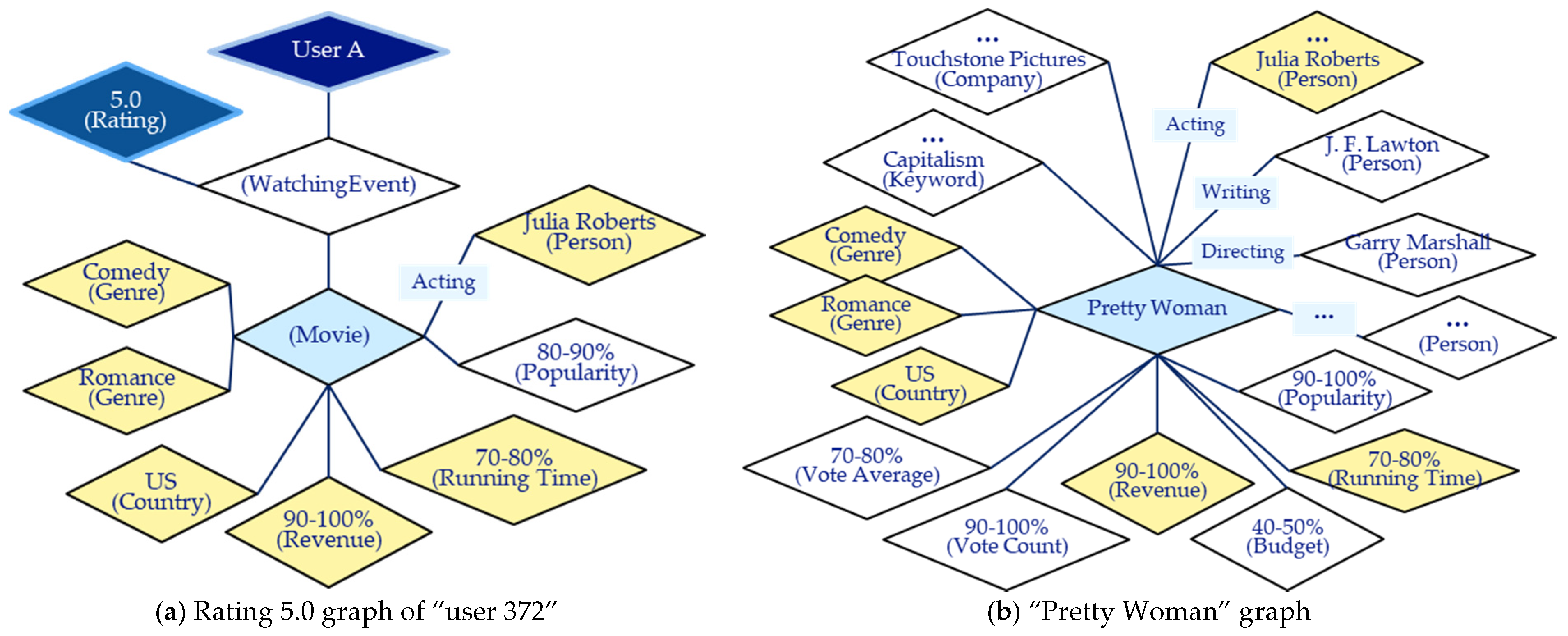
In addition to the performance of the movie rating prediction described so far, the frequent subgraph derived from the experiment contains knowledge to explain to the user why our methodology predicts that the movie will be rated at 5.0. Figure 26 shows the frequent subgraph (i.e., the rating 5.0 graph) of “user 372” derived from the training set used in the experiment and target movie (“Pretty Woman”) graph to be predicted that the user gives a rating of 5.0.

Between the “rating 5.0 graph” from “user 372”‘s past history and “Pretty Woman” graph, there are attributes in common such as “Julia Roberts” as an actor, “comedy” and “romance” in genre, “US” in film making country, revenue in 90–100% of all movies used in the experiment, and running time in 70–80% of all movies. With common factors described above we can explain why our methodology predicts that “user 372” will give a rating of 5.0 for “Pretty Woman.” In particular, users do not intuitively know their preferences for features such as revenue or running time. However, the fact that these features can also be presented as a basis for prediction is a major feature of this study.

4. Discussion

With a continuous increase in the quantity of newly generated information, tools and environments for amassing and utilizing information in the form of ontology-based knowledge graphs are increasing in usefulness and scope of application. Therefore, researchers across various fields are exploring diverse techniques to extract meaningful information from the accumulated knowledge. That is, vast quantities of information, including user activity on general web sites, purchase history and item viewing history on online stores, and viewing and playback history on movie and music websites, do not exist only in the form of raw data but are accumulated as components of structured knowledge graphs. This study primarily aimed to efficiently find frequent patterns in these enormous knowledge graphs, which were verified through experiments that determined how well these frequent patterns represented the graph to which they belonged (in this case, the user).

In this study, we used Resource Description Framework (RDFS) and Web Ontology Language (OWL) to represent our ontology. We newly designed the schema of this movie ontology and created the knowledge graph by combining the user’s rating record and movie information. Since these original data were in a rather simple form (tables), we could easily represent our movie ontology at a relatively light level without using a language with rich expressiveness. In the future, we need to think about how to deal with complex and detailed ontology expressions such as inter-class relationships.

The actual experiments were performed on a notebook with an Intel^® Core™ i5-1035G7 CPU@ 1.2GHz processor with 16 GB of RAM running on Windows 64-bit. We implemented our methodology using Java in frequent subgraph mining and using Python in movie rating prediction. When implementing frequent subgraph mining, we tried to reduce computational time by creating temporal tables during the computation process and directly hashing reference to the data in these tables. In the process of basic exploration and frequency counting, the frequency of all triples was calculated in advance, stored in memory and used in candidate generation. We also created a table for triples in each chunking step and used it to finally reconstruct a frequent subgraph.

Considering time complexity among computational complexity, time-consuming operations in our methodology are performed in two major parts. The first is the process of finding all paths between the start class and the end classes in the ontology graph. In this case, the commonly used DFS was utilized, and time complexity is $O\left(\left|class\right|+\left|property\right|\right)$. The second is the process of finding the same triple in a single table consisting of instance triples, which, in the worst case, requires $n\left(n-1\right)$ iterations, when the number of instance triples is $n$. Therefore, even if the “visited” flag was used, the time complexity is $O\left(n^2\right)$. For space complexity, the size of the input data used in the experiment is about 300 MB, and the memory used during the frequent subgraph mining is about 1.2 GB.

Regarding the threshold used in the process of generating the candidates subject to chunking, it is necessary to research general criteria that can be applied in fields with different data characteristics. For example, the main factors that should be considered include the number of instances in the knowledge graph, the number of instance triples, or the length and number of instance triple paths.

It is also necessary to research the chunking priority in future studies. In this study, small subgraphs were prioritized for chunking if the frequencies were the same; however, chunking the larger graph first may show better or worse performance. The chunking priority needs to be determined to reflect the characteristics of the target knowledge graph well and a study related to this is needed.

Meanwhile, in terms of rating prediction, in place of the current method utilizing graph similarity, a future study will be conducted on a method utilizing neural networks by embedding the frequent patterns through matrix factorization.

5. Conclusions

This study first decomposed a large-scale ontology graph into small unit subgraphs, used these as units to calculate the frequency of the instance triples (or chunks), and made a chunk to find the frequent subgraphs. Next, the similarity between the rating graph and item graph was calculated via a Levenshtein distance-based method to predict the rating. The proposed approach was applied to an actual movie rating dataset and compared with other recommendation methods. According to the results, it outperformed the other approaches by approximately 40% in terms of accuracy and slightly outperformed them in terms of the F1-score, thus demonstrating that the proposed methodology can be useful in real applications.

The main contributions of this study are as follows:

• This study presented a novel method of decomposing a large-scale knowledge graph into small unit subgraphs. These unit subgraphs serve as the criterion for occurrence counting, thereby enabling the frequency to be efficiently calculated. This approach of generating unit subgraphs to mine frequent subgraphs maintains the graph structure and meaning, which differentiates it from the method of simply creating transactions through an item set to apply an association rule mining algorithm.
• The process starts with one instance triple and expands the subgraph through chunking. This chunking method makes it possible to find larger patterns while maintaining the structural information of the subgraph. By employing a method that utilizes instance triple paths, the subgraph can be expanded without being significantly affected by the size of the knowledge graph by performing chunking with a chunk and instance triple or between chunks.
• Rather than merely extracting the frequent subgraphs, the methodology was applied to the application area of rating prediction. Its feasibility in providing recommendations through rating prediction was demonstrated, thus empirically proving the usefulness of frequent subgraphs. That is, the approach was shown to be effective when compared with other collaborative filtering algorithms, and a method for confirming the significance of the extracted frequent pattern was presented.
• The proposed methodology can be used as a general recommendation engine extending the scope of the movie rating prediction. Information such as a user’s purchasing history, areas of interest, and personal profiles acquired at the time of subscription can be represented in a graph, and then the proposed methodology can be used as a tool to analyze the buying patterns of other users with similar purchasing histories. In addition, the proposed methodology can also demonstrate high utilization in natural language processing such as complex questioning and natural language generation, and anomaly detection, which monitors and controls anomalies in real time by modeling complex structured networks, IT equipment and software in graph form, is a suitable field to show the performance of our methodology. On the other hand, our methodology is expected that in the bioscience area where the data involved is often represented by knowledge graphs, it will be able to demonstrate good performance in analyzing what proteins cause disease, what their relationship is, or whether certain drugs react to certain proteins in the human body and affect lesions.

The extracted frequent subgraph maintains the original semantic information. The extensively researched rating prediction or recommendation approaches have the disadvantage of being unable to provide a reason or explanation for the result, which will likely be challenging to solve in future related studies as well. However, the methodology of this study has the significant advantage of being able to provide a clear answer to questions such as “Why do you predict that I will give this movie a 4.0 rating?” or “Why are you recommending this movie to me?”