
Long Term Effects of Forest Liming on the Acid-Base Budget


Abstract
1. Introduction
2. Materials and Methods
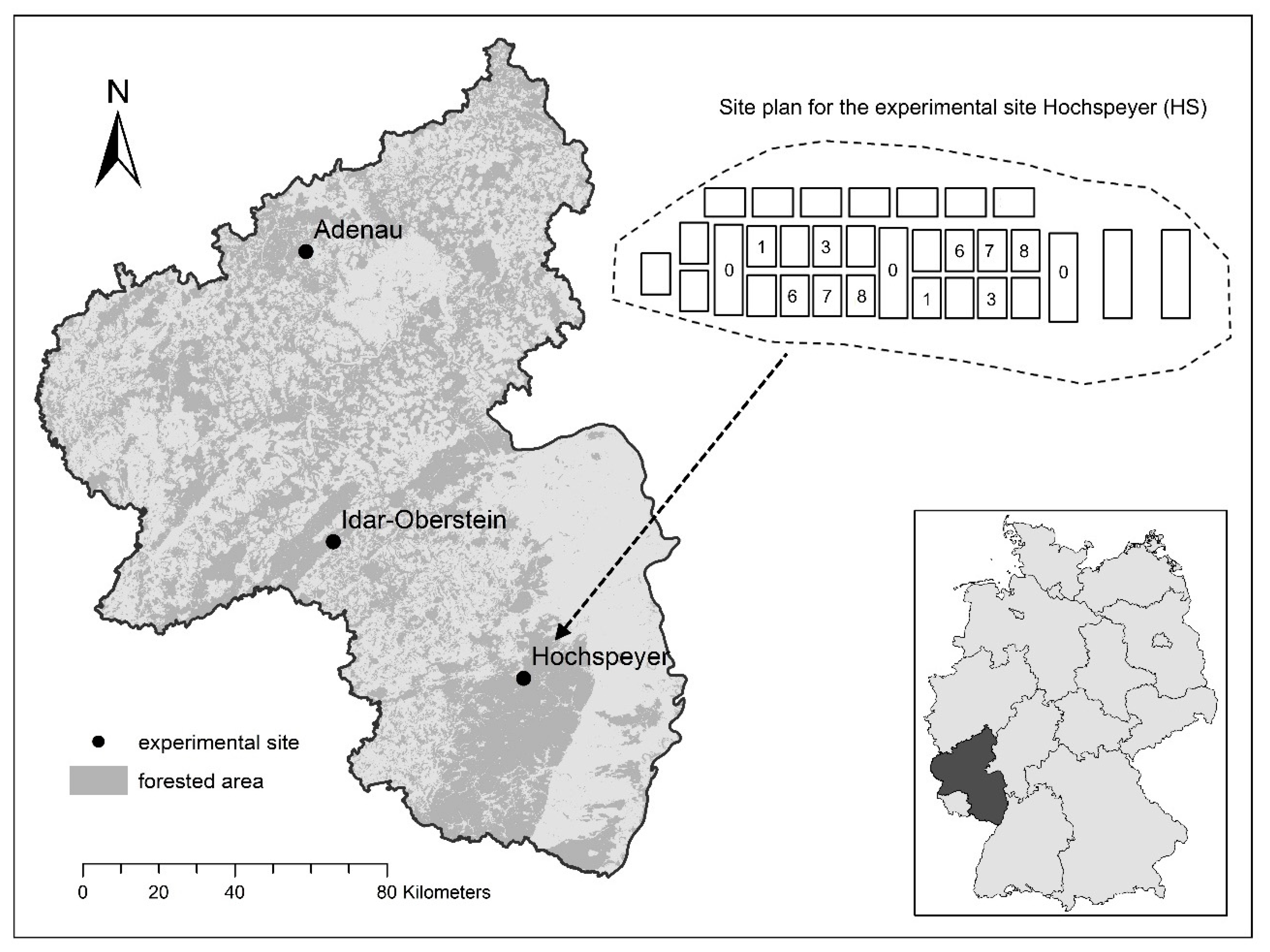
2.1. Sites
2.2. Element Fluxes
2.3. Calculation of Acid-Base Budgets
2.4. Modification of the Original Approach
3. Results
3.1. Site Characteristics
3.2. Effect of Liming Treatments
4. Discussion
Author Contributions
Funding
Institutional Review Board Statement
Informed Consent Statement
Data Availability Statement
Acknowledgments
Conflicts of Interest
References
- Ulrich, B. Die Rolle der Bodenversauerung beim Waldsterben: Langfristige Konsequenzen und forstliche Möglichkeiten. Forstwiss. Cent. 1986, 105, 421–435. [Google Scholar] [CrossRef]
- Ulrich, B.; Mayer, R.; Khanna, P.K. Deposition von Luftverunreinigungen und Ihre Auswirkungen in Waldökosystemen im Solling; Schriftenreihe der Forstlichen Fakultät der Universität Göttingen: Göttingen, Germany, 1979; Volume 58. [Google Scholar]
- Alewell, C.; Manderscheid, B.; Gerstberger, P.; Matzner, E. Effects of reduced atmospheric deposition on soil solution chemistry and elemental contents of spruce needles in NE-Bavaria, Germany. J. Plant Nutr. Soil Sci. 2000, 163, 509–516. [Google Scholar] [CrossRef]
- Waldner, P.; Marchetto, A.; Thimonier, A.; Schmitt, M.; Rogora, M.; Granke, O.; Mues, V.; Hansen, K.; Pihl Karlsson, G.; Žlindra, D.; et al. Detection of temporal trends in atmospheric deposition of inorganic nitrogen and sulphate to forests in Europe. Atmos. Environ. 2014, 95, 363–374. [Google Scholar] [CrossRef]
- Stoddard, J.; Jeffries, D.; Lükewille, A.; Clair, T.; Dillon, P.; Driscoll, C.T.; Forsius, M.; Johannessen, M.; Kahl, J.S.; Kellogg, J.; et al. Regional trends in aquatic recovery from acidification in North America and Europe. Nature 1999, 401, 575–578. [Google Scholar] [CrossRef]
- European Environment Agency Air Pollution Fact Sheet 2014: Germany. Available online: http://www.eea.europa.eu/themes/air/air-pollution-country-fact-sheets-2014/germany-air-pollutant-emissions-country-factsheet (accessed on 21 January 2021).
- Umweltbundesamt Ammoniak-Emissionen—Entwicklung Seit 1990. Available online: http://www.umweltbundesamt.de/daten/luftbelastung/luftschadstoff-emissionen-in-deutschland/ammoniak-emissionen (accessed on 21 January 2021).
- Meesenburg, H.; Eichhorn, J.; Meiwes, K.J. Atmospheric Deposition and Canopy Interactions. In Functioning and Management of European Beech Ecosystems; Brumme, R., Khanna, P.K., Eds.; Ecological Studies 208; Springer: Berlin/Heidelberg, Germany, 2009; pp. 265–302. [Google Scholar]
- Meiwes, K.J. Application of lime and wood ash to decrease acidification of forest soils. Water Air Soil Pollut. 1995, 85, 143–152. [Google Scholar] [CrossRef]
- Ebermayer, E. Die Gesammte Lehre der Waldstreu Mit Rücksicht auf die Chemische Statik des Waldbaues; Julius Springer: Berlin/Heidelberg, Germany, 1876. [Google Scholar]
- Block, J.; Gauer, J. Waldbodenzustand in Rheinland-Pfalz; Mitteilungen aus der Forschungsanstalt für Waldökologie und Forstwirtschaft Rheinland-Pfalz: Trippstadt, Germany, 2012; Volume 70. [Google Scholar]
- Dise, N.B.; Matzner, E.; Armbruster, M.; MacDonald, J. Aluminum output fluxes from forest ecosystems in Europe: A regional assessment. J. Environ. Qual. 1994, 30, 1747–1756. [Google Scholar] [CrossRef]
- Ulrich, B. Natural and anthropogenic components of soil acidification. Z. Pflanzenernähr. Bodenkd. 1986, 149, 702–717. [Google Scholar] [CrossRef]
- Van Breemen, N.; Mulder, J.; Driscoll, C.T. Acidification and alkalinization of soils. Plant Soil 1983, 75, 283–308. [Google Scholar] [CrossRef]
- Butz-Braun, R. Einfluss der Bodenschutzkalkung auf den Entwicklungszustand der Tonminerale. Forstarchiv 2014, 85, 65–67. [Google Scholar] [CrossRef]
- Hüttl, R.F.; Zöttl, H.W. Liming as a mitigation tool in Germany’s declining forests—Reviewing results from former and recent trials. For. Ecol. Manag. 1993, 61, 325–338. [Google Scholar] [CrossRef]
- Schüler, G. Schutz versauerter Böden in nachhaltig bewirtschafteten Wäldern-Ergebnisse aus 10-jähriger interdisziplinärer Forschung. Allg. Forst Jagdztg. 2002, 173, 1–7. [Google Scholar]
- Gussone, H.A. Empfehlungen zur Kompensationsdüngung. Forst Holzwirt 1984, 6, 154–160. [Google Scholar]
- Schüler, G. Der Vergleichende Kompensationsversuch mit Verschiedenen Puffersubstanzen zur Minderung der Auswirkungen von Luftschadstoffeinträgen in Waldökosystemen; Mitteilungen aus der Forstlichen Versuchsanstalt Rheinland-Pfalz: Trippstadt, Germany, 1992; Volume 21. [Google Scholar]
- Veerhoff, M.; Brümmer, G.W. Silicatverwitlerung und -zerstörung in Waldböden als Folge von Versauerungsprozessen und deren ökologische Konsequenzen. Nat. Landsch. 1992, 28, 25–32. [Google Scholar]
- Gutachterausschuss Forstliche Analytik. Handbuch Forstliche Analytik; Gutachterausschuss Forstliche Analytik: Göttingen, Germany, 2009. [Google Scholar]
- Greve, M. Langfristige Auswirkungen der Waldkalkung auf den Stoffhaushalt; Mitteilungen aus der Forschungsanstalt für Waldökologie und Forstwirtschaft Rheinland-Pfalz: Trippstadt, Germany, 2015; Volume 73. [Google Scholar]
- Karl, S.; Block, J.; Schüler, G.; Schultze, B.; Scherzer, J. Wasserhaushaltsuntersuchungen im Rahmen des Forstlichen Umweltmonitorings und bei Waldbaulichen Versuchen in Rheinland-Pfalz; Mitteilungen aus der Forschungsanstalt für Waldökologie und Forstwirtschaft Rheinland-Pfalz: Trippstadt, Germany, 2012; Volume 71. [Google Scholar]
- Ellenberg, H.; Mayer, R.; Schauermann, J. Ökosystemforschung. Ergebnisse des Sollingprojekts 1966–1986; Ulmer Eugen Verlag: Stuttgart, Germany, 1986; ISBN 978-3800134311. [Google Scholar]
- Berger, T.W.; Untersteiner, H.; Toplitzer, M.; Neubauer, C. Nutrient fluxes in pure and mixed stands of spruce (Picea abies) and beech (Fagus sylvatica). Plant Soil 2009, 322, 317–342. [Google Scholar] [CrossRef]
- Ulrich, B. Nutrient and acid-base budget of central European forest ecosystems. In Effects of Acid Rain on Forest Processes; Godbold, D.L., Hüttermann, A., Eds.; Wiley-Liss: New York, NY, USA, 1994; pp. 1–50. ISBN 9780471517689. [Google Scholar]
- Draaijers, G.P.J.; Erisman, J.W. A canopy budget model to assess atmospheric deposition from throughfall measurements. Water Air Soil Pollut. 1995, 85, 2253–2258. [Google Scholar] [CrossRef]
- Meesenburg, H.; Mohr, K.; Dämmgen, U.; Schaaf, S.; Meiwes, K.J.; Horváth, B. Stickstoff-Einträge und -Bilanzen in den Wäldern des ANSWER-Projektes: Eine Synthese. Landbauforsch. Völkenrode Sonderh. 2005, 279, 95–108. [Google Scholar]
- Sverdrup, H.; Warfvinge, P.E.R. Calculating field weathering rates using a mechanistic geochemical model PROFILE. Appl. Geochem. 1993, 8, 273–283. [Google Scholar] [CrossRef]
- Becker, R. Critical Load-PROFILE 4.4 (Manual); ÖKO-DATA Strausberg: Brandenburg, Germany, 2002. [Google Scholar]
- Watson, C. Seasonal soil temperature regimes in south-eastern Australia. Aust. J. Soil Res. 1980, 18, 325. [Google Scholar] [CrossRef]
- Stephens, J.C. Response of Soil Mineral Weathering to Elevated Carbon Dioxide. Ph.D. Thesis, California Institute of Technology, Pasadena, CA, USA, 2002. [Google Scholar]
- Golubev, S.V.; Pokrovsky, O.S.; Schott, J. Experimental determination of the effect of dissolved CO2 on the dissolution kinetics of Mg and Ca silicates at 25 °C. Chem. Geol. 2005, 217, 227–238. [Google Scholar] [CrossRef]
- Brantley, S.L. Kinetics of Water-Rock Interaction. In Kinetics of Water-Rock Interaction; Brantley, S.L., Kubicki, J.D., White, A.F., Eds.; Springer: New York, NY, USA, 2008; pp. 151–210. ISBN 978-0-387-73562-7. [Google Scholar]
- Pretzsch, H.; Biber, P.; Ďurský, J. The single tree-based stand simulator SILVA: Construction, application and evaluation. For. Ecol. Manag. 2002, 162, 3–21. [Google Scholar] [CrossRef]
- Pretzsch, H.; Block, J.; Dieler, J.; Schuck, J.; Gauer, J.; Göttlein, A.; Moshammer, R.; Weis, W.; Wunn, U. Nährstoffentzüge durch die Holz- und Biomassenutzung in Wäldern. Teil 1: Schätzfunktionen für Biomasse und Nährelemente und ihre Anwendung in Szenariorechnungen. Allg. Forst Jagdztg. 2014, 185, 261–285. [Google Scholar]
- Pretzsch, H.; Block, J.; Böttcher, M.; Dieler, J.; Gauer, J.; Göttlein, A.; Moshammer, R.; Schuck, J.; Weis, W.; Wunn, U. Entscheidungsstützungssystem zum Nährstoffentzug im Rahmen der Holzernte: Nährstoffbilanzen Wichtiger Waldstandorte in Bayern und Rheinland-Pfalz. Abschlussbericht zum DBU-Projekt Az. 25966-33/0. 2013. Available online: https://fawf.wald-rlp.de/de/veroeffentlichungen/projektberichte/ (accessed on 21 January 2021).
- Ulrich, B. Rechenweg zur Schätzung der Flüsse in Waldökosystemen: Identifizierung der sie Bedingenden Prozesse; Berichte des Forschungszentrums Waldökosysteme Göttingen, Reihe B; Berichte des Forschungszentrums Waldökosysteme Göttingen: Göttingen, Germany, 1991; Volume 24. [Google Scholar]
- Mosello, R.; Amoriello, T.; Benham, S.; Clarke, N.; Derome, J.; Derome, K.; Genouw, G.; Koenig, N.; Orrù, A.; Tartari, G.; et al. Validation of chemical analyses of atmospheric deposition on forested sites in Europe: 2. DOC concentration as an estimator of the organic ion charge. J. Limnol. 2008, 67, 1–14. [Google Scholar] [CrossRef]
- ICP Forests New Excel File for Analytical Data Validation (with DOC). Available online: http://storage.ning.com/topology/rest/1.0/file/get/118302774?profile=original (accessed on 21 January 2021).
- Van Breemen, N.; Driscoll, C.T.; Mulder, J. Acidic deposition and internal proton sources in acidification of soils and waters. Nature 1984, 307, 599–604. [Google Scholar] [CrossRef]
- Greve, M. Langfristige Auswirkungen der Waldkalkung auf Bodenzustand, Sickerwasser und Nadelspiegelwerte von drei Versuchsanlagen in Rheinland-Pfalz. Forstarchiv 2014, 46, 35–46. [Google Scholar] [CrossRef]
- Block, J.; Roeder, A.; Schüler, G. Waldbodenrestauration durch Aktivierung ökosystemarer Nährstoffkreisläufe. Allg. For. Z. 1997, 52, 29–33. [Google Scholar]
- Veerhoff, M.; Brümmer, G. Silicatverwitterung und Tonmineralumwandlung in Waldböden als Folge von Versauerungsprozessen. Mitt. Deutsch. Bodenkd. Gese. 1989, 59, 1203–1207. [Google Scholar]
- Gjengedal, E.; Martinsen, T.; Steinnes, E. Background levels of some major, trace, and rare earth elements in indigenous plant species growing in Norway and the influence of soil acidification, soil parent material, and seasonal variation on these levels. Environ. Monit. Assess. 2015, 187. [Google Scholar] [CrossRef]
- Ducić, T.; Parladé, J.; Polle, A. The influence of the ectomycorrhizal fungus Rhizopogon subareolatus on growth and nutrient element localisation in two varieties of Douglas fir (Pseudotsuga menziesii var. menziesii and var. glauca) in response to manganese stress. Mycorrhiza 2008, 18, 227–239. [Google Scholar] [CrossRef]
- De Wit, H.A.; Eldhuset, T.D.; Mulder, J. Dissolved Al reduces Mg uptake in Norway spruce forest: Results from a long-term field manipulation experiment in Norway. For. Ecol. Manag. 2010, 259, 2072–2082. [Google Scholar] [CrossRef]
- Poschenrieder, C.; Gunsé, B.; Corrales, I.; Barceló, J. A glance into aluminum toxicity and resistance in plants. Sci. Total Environ. 2008, 400, 356–368. [Google Scholar] [CrossRef]
- Chen, D.; Lan, Z.; Hu, S.; Bai, Y. Effects of nitrogen enrichment on belowground communities in grassland: Relative role of soil nitrogen availability vs. soil acidification. Soil Biol. Biochem. 2015, 89, 99–108. [Google Scholar] [CrossRef]
- Butz-Braun, R. Beprobung und Mineralogische Analysen an dem Vergleichenden Kompensationsversuch Idar-Oberstein, dem Bodenrestaurationsversuch Pirmasens und der UKS Merzalben. Forschungsbericht für die Forschungsanstalt für Waldökologie und Forstwirtschaft. 2012. Available online: https://fawf.wald-rlp.de/de/veroeffentlichungen/projektberichte/ (accessed on 21 January 2021).
- Butz-Braun, R. Tonmineralogische Untersuchungen zum Kompensationsversuch 2010 Versuchsanlage Adenau (101)—3. Detaillierte Wiederholung—Ergänzung um die 15 t Dolomit-Variante. Forschungsbericht für die Forschungsanstalt für Waldökologie und Forstwirtschaft. 2011. Available online: https://fawf.wald-rlp.de/de/veroeffentlichungen/projektberichte/ (accessed on 21 January 2021).
- Butz-Braun, R. Tonmineralogische Untersuchungen zum Kompensationsversuch 2007 und 2012 Versuchsanlage Hochspeyer (318)—2. und 3. Wiederholung. Forschungsbericht für die Forschungsanstalt für Waldökologie und Forstwirtschaft. 2012. Available online: https://fawf.wald-rlp.de/de/veroeffentlichungen/projektberichte/ (accessed on 21 January 2021).
- Prenzel, J.; Meiwes, K.J. Sulfate Sorption in Soils under Acid Deposition: Modeling Field Data from Forest Liming. J. Environ. Qual. 1994, 23, 1212–1217. [Google Scholar] [CrossRef]
- Alewell, C. Predicting reversibility of acidification: The European sulfur story. Water Air Soil Pollut. 2001, 130, 1271–1276. [Google Scholar] [CrossRef]
- Block, J.; Eichhorn, J.; Gehrmann, J.; Kölling, C.; Matzner, E.; Meiwes, K.J.; von Wilpert, K.; Wolff, B. Kennwerte zur Charakterisierung des Ökochemischen Bodenzustandes und des Gefährdungspotentials Durch Bodenversauerung und Stickstoffsättigung an Level II-Waldökosystem-Dauerbeobachtungsflächen. Arbeitskreis C der Bund-Länder-Arbeitsgruppe Level II; Bundesministerium für Ernährung, Landwirtschaft und Forsten (BMELF): Bonn, Germany, 2000. [Google Scholar]
- Bittersohl, J.; Walther, W.; Meesenburg, H. Gewässerversauerung durch Säuredeposition in Deutschland—Entwicklung und aktueller Stand. Hydrol. Wasserbewirtsch. 2014, 58, 260–273. [Google Scholar] [CrossRef]
- Marschner, H.; Häussling, M.; George, E. Ammonium and nitrate uptake rates and rhizosphere pH in non-mycorrhizal roots of Norway spruce [Picea abies (L.) Karst.]. Trees 1991, 5, 14–21. [Google Scholar] [CrossRef]
- Buchmann, N.; Schulze, E.-D.; Gebauer, G. 15N-ammonium and 15N-nitrate uptake of a 15-year-old Picea abies plantation. Oecologia 1995, 102, 361–370. [Google Scholar] [CrossRef]
- Gessler, A.; Schneider, S.; Von Sengbusch, D.; Weber, P.; Hanemann, U.; Huber, C.; Rothe, A.; Kreutzer, K.; Rennenberg, H. Field and laboratory experiments on net uptake of nitrate and ammonium by the roots of spruce (Picea abies) and beech (Fagus sylvatica) trees. New Phytol. 1998, 138, 275–285. [Google Scholar] [CrossRef]
- Anttonen, S.; Manninen, A.-M.; Saranpää, P.; Kainulainen, P.; Linder, S.; Vapaavuori, E. Effects of long-term nutrient optimisation on stem wood chemistry in Picea abies. Trees 2002, 16, 386–394. [Google Scholar] [CrossRef]
- Feng, Z. Partitioning of Atmospheric Nitrogen under Long-Term Reduced Atmospheric Deposition Conditions in a Norway Spruce Forest Ecosystem; Göttinger Forstwissenschaften; Universitätsverlag Göttingen: Göttingen, Germany, 2010; Volume 4. [Google Scholar]
- Kopáček, J.; Hejzlar, J.; Kaňa, J.; Porcal, P.; Turek, J. The sensitivity of water chemistry to climate in a forested, nitrogen-saturated catchment recovering from acidification. Ecol. Indic. 2016, 63, 196–208. [Google Scholar] [CrossRef]


| Study Areas | Adenau (AD) | Idar-Oberstein (IO) | Hochspeyer (HS) |
|---|---|---|---|
| Elevation above mean sea level | 580–630 m | 540–550 m | 385–400 m |
| Coordinates (ETRS 1989 UTM32N) | X: 364340 Y: 5588220 | X: 371450 Y: 5512000 | X: 421560 Y: 5476010 |
| Slope (Degree) | 7° | 4° | 3° |
| Mean annual temperature | 7.6 °C | 8.3 °C | 8.7 °C |
| Mean annual temperature of the vegetation period | 12.6 °C | 13.3 °C | 14.5 °C |
| Mean annual precipitation | 850 mm | 1065 mm | 770 mm |
| Seepage (60 cm) | 275 mm | 310 mm | 180 mm |
| Parent material | Diluvial loam above devonic quarzite | Diluvial loam above devonic quarzite | Sandstone of the bunter sandstone |
| Soil Taxonomy (WRB) | Cambisol | Stagnic cambisol | Podzol |
| Humus form | Mor humus | Mor humus | Raw humus |
| Soil texture | Clay loam | Clay loam | Loamy Sand |
| pH(CaCl2): 0–10/20–30 cm | 2.9/3.9 | 3.0/4.0 | 2.9/3.6 |
| Base saturation: 0–10/20–30 cm | 7.2%/2.8% | 6.3%/4.6% | 10.3%/5.5% |
| Cation exchange capacity [µeq g−1]: 0–10/20–30 cm | 139/46 | 137/47 | 103/19 |
| C content [g kg−1]: 0–10/20–30 cm | 65.8/12.7 | 75.0/12.1 | 72.8/10.7 |
| N content [g kg−1]: 0–10/20–30 cm | 3.1/1.3 | 3.7/1.1 | 2.7/0.5 |
| S content [g kg−1]: 0–10/20–30 cm | 1.49/0.38 | 1.21/0.46 | 0.58/0.19 |
| Tree species | Picea abies | Picea abies | Pinus sylvestris mixed with Fagus sylvatica from natural regeneration |
| Stand age (2016) | 81 | 97 | 90/96 (Pinus sylvestris) |
| LT | Lime and Fertilizer Application | Mg [kg ha−1] | Ca [kg ha−1] | K [kg ha−1] | P [kg ha−1] | S [kg ha−1] | ANC [keq ha−1] | Additional Informations |
|---|---|---|---|---|---|---|---|---|
| 0 | - | - | - | control plot, no treatment | ||||
| 1 | Dolomite: 3000 kg ha−1 | 349 | 603 | 51 | particle size 0–2 mm | |||
| 3 | Dolomite: 3000 kg ha−1 | 349 | 603 | 53 | particle size 0–2 mm | |||
| Hyperphos: 330 kg ha−1 | 6 | 96 | 6 | 37 | Soft ground rock phosphate | |||
| 6 | Dolomite: 5000 kg ha−1 | 582 | 1005 | 85 | particle size 0–2 mm | |||
| 7 | Dolomite: 9000 kg ha− | 1048 | 1809 | 153 | particle size 0–2 mm | |||
| Patentkali: 340 kg ha−1 | 21 | 85 | 58 | as K2SO4 and MgSO4 | ||||
| Kieserite: 660 kg ha−1 | 107 | 145 | as MgSO4 | |||||
| 8 | Mixture of Dolomite and Hyperphos: 15,000 kg ha−1 | 1441 | 3804 | 25 | 145 | 304 | particle size 0–0.09 mm mixed with soft ground rock phosphate |
| Proton Production [keq ha−1 24a−1] | Proton Consumption [keq ha−1 24a−1] | Portion | |||||||||||||||||||
|---|---|---|---|---|---|---|---|---|---|---|---|---|---|---|---|---|---|---|---|---|---|
| Site | Liming Treatment | Subplot | H+ | NH4+ | NO3− | SO42− | Org− | Ma | Mb | ∑ | Diff. | ∑ | H+ | NH4+ | NO3− | SO42− | Org− | Ma | Mb | Ma | Mb |
| AD | 0 | 1 | 5.4 | 31.1 | 0.2 | 5.8 | 6.6 | 0.1 | 5.5 | 54.6 | 0.6 | 54.0 | 1.2 | 0.0 | 18.5 | 2.0 | 0.0 | 29.9 | 2.5 | 55% | 5% |
| 0 | 2 | 6.5 | 31.1 | 1.8 | 4.0 | 4.3 | 0.1 | 5.6 | 53.4 | −0.7 | 54.1 | 0.7 | 0.0 | 6.5 | 3.6 | 0.0 | 40.1 | 3.2 | 74% | 6% | |
| 1 | 1 | 6.0 | 31.4 | 4.5 | 13.8 | 7.2 | 0.1 | 4.5 | 67.5 | −1.2 | 68.7 | 0.7 | 0.0 | 8.6 | 0.4 | 0.0 | 34.0 | 24.9 | 50% | 36% | |
| 1 | 2 | 6.3 | 31.0 | 7.9 | 22.3 | 6.0 | 0.1 | 3.9 | 77.6 | −2.5 | 80.1 | 0.8 | 0.0 | 1.7 | 0.5 | 0.0 | 39.3 | 37.7 | 49% | 47% | |
| 3 | 1 | 6.4 | 30.7 | 2.4 | 9.5 | 6.9 | 0.1 | 4.4 | 60.3 | 0.1 | 60.2 | 1.6 | 0.0 | 7.7 | 1.2 | 0.0 | 35.9 | 13.9 | 60% | 23% | |
| 3 | 2 | 5.6 | 31.4 | 1.5 | 3.7 | 10.2 | 0.0 | 3.7 | 56.1 | −0.5 | 56.5 | 1.0 | 0.0 | 7.5 | 3.4 | 0.0 | 29.3 | 15.4 | 52% | 27% | |
| 6 | 1 | 6.3 | 31.5 | 9.2 | 11.3 | 7.1 | 0.1 | 4.2 | 69.7 | 0.2 | 69.5 | 0.6 | 0.0 | 1.3 | 1.9 | 0.0 | 35.8 | 29.9 | 52% | 43% | |
| 6 | 2 | 5.0 | 31.0 | 22.3 | 15.5 | 11.0 | 0.0 | 3.2 | 88.0 | −2.3 | 90.4 | 1.2 | 0.0 | 1.3 | 0.9 | 0.0 | 38.6 | 48.4 | 43% | 54% | |
| 7 | 1 | 6.0 | 31.4 | 26.0 | 26.6 | 11.1 | 0.0 | 3.6 | 104.8 | −5.5 | 110.3 | 0.9 | 0.0 | 0.0 | 0.6 | 0.0 | 44.5 | 64.3 | 40% | 58% | |
| 7 | 2 | 6.7 | 31.3 | 10.9 | 29.1 | 9.4 | 0.0 | 5.1 | 92.5 | −4.8 | 97.2 | 0.9 | 0.0 | 5.9 | 1.0 | 0.0 | 47.0 | 42.5 | 48% | 44% | |
| 8 | 1 | 7.1 | 31.6 | 7.1 | 14.7 | 10.0 | 0.0 | 3.5 | 74.0 | −2.6 | 76.6 | 0.4 | 0.0 | 1.9 | 1.7 | 0.0 | 26.0 | 46.6 | 34% | 61% | |
| 8 | 2 | 6.5 | 31.3 | 9.9 | 14.2 | 9.0 | 0.1 | 3.3 | 74.2 | −1.7 | 75.9 | 0.5 | 0.0 | 3.7 | 1.2 | 0.0 | 25.7 | 44.7 | 34% | 59% | |
| IO | 0 | 1 | 13.8 | 13.7 | 0.0 | 18.3 | 2.5 | 0.2 | 5.7 | 54.1 | −5.7 | 59.8 | 0.0 | 0.0 | 20.8 | 0.3 | 0.0 | 35.0 | 3.7 | 58% | 6% |
| 0 | 2 | 13.8 | 13.7 | 0.0 | 34.7 | 3.3 | 0.2 | 3.0 | 68.7 | −6.7 | 75.4 | 0.0 | 0.0 | 17.6 | 0.0 | 0.0 | 46.5 | 11.3 | 62% | 15% | |
| 1 | 1 | 15.0 | 13.7 | 0.0 | 18.9 | 2.9 | 0.1 | 3.9 | 54.6 | −6.5 | 61.1 | 0.0 | 0.0 | 21.4 | 0.5 | 0.0 | 30.2 | 9.1 | 49% | 15% | |
| 1 | 2 | 14.9 | 13.7 | 0.0 | 32.2 | 3.6 | 0.1 | 2.3 | 66.8 | −6.2 | 73.0 | 0.0 | 0.0 | 14.3 | 0.0 | 0.0 | 31.6 | 27.2 | 43% | 37% | |
| 3 | 1 | 13.8 | 13.7 | 7.3 | 34.0 | 3.7 | 0.1 | 1.6 | 74.2 | −7.7 | 81.9 | 0.0 | 0.0 | 14.7 | 0.1 | 0.0 | 39.8 | 27.3 | 49% | 33% | |
| 3 | 2 | 15.8 | 13.7 | 0.0 | 13.8 | 1.6 | 0.1 | 4.1 | 49.1 | −6.9 | 56.0 | 0.0 | 0.0 | 21.1 | 0.6 | 0.0 | 27.7 | 6.6 | 49% | 12% | |
| 6 | 1 | 14.7 | 13.5 | 2.2 | 29.6 | 9.7 | 0.1 | 0.8 | 70.6 | −10.4 | 81.0 | 0.0 | 0.0 | 12.4 | 0.0 | 0.0 | 27.3 | 41.3 | 34% | 51% | |
| 6 | 2 | 15.3 | 13.7 | 0.0 | 30.6 | 3.1 | 0.1 | 1.9 | 64.7 | −7.1 | 71.8 | 0.0 | 0.0 | 17.3 | 0.3 | 0.0 | 26.9 | 27.3 | 38% | 38% | |
| 7 | 1 | 15.2 | 13.8 | 0.1 | 29.1 | 2.5 | 0.1 | 2.3 | 63.2 | −6.9 | 70.2 | 0.0 | 0.0 | 17.4 | 0.0 | 0.0 | 30.9 | 21.9 | 44% | 31% | |
| 7 | 2 | 15.4 | 13.5 | 0.3 | 38.3 | 6.7 | 0.1 | 0.7 | 75.1 | −6.1 | 81.1 | 0.0 | 0.0 | 13.0 | 0.0 | 0.0 | 25.4 | 42.7 | 31% | 53% | |
| 8 | 1 | 15.8 | 13.8 | 0.1 | 25.7 | 2.7 | 0.2 | 2.5 | 60.8 | −6.5 | 67.3 | 0.0 | 0.0 | 15.3 | 0.2 | 0.0 | 23.0 | 28.8 | 34% | 43% | |
| 8 | 2 | 15.9 | 13.8 | 0.0 | 31.0 | 4.0 | 0.1 | 1.4 | 66.2 | −5.5 | 71.8 | 0.0 | 0.0 | 18.7 | 0.6 | 0.0 | 20.5 | 31.9 | 29% | 45% | |
| HS | 0 | 1 | 2.9 | 11.1 | 0.0 | 0.5 | 16.5 | 0.1 | 2.8 | 33.8 | −3.8 | 37.6 | 0.5 | 0.0 | 14.3 | 2.0 | 0.0 | 18.2 | 2.6 | 48% | 7% |
| 0 | 2 | 5.9 | 11.2 | 0.0 | 3.3 | 3.1 | 0.2 | 3.3 | 27.0 | −2.8 | 29.7 | 0.0 | 0.0 | 14.3 | 0.1 | 0.0 | 13.4 | 1.9 | 45% | 6% | |
| 1 | 1 | 5.1 | 11.2 | 0.0 | 1.0 | 16.4 | 0.1 | 1.5 | 35.2 | −6.3 | 41.5 | 0.0 | 0.0 | 14.3 | 1.6 | 0.0 | 20.0 | 5.6 | 48% | 13% | |
| 1 | 2 | 4.6 | 11.1 | 0.0 | 2.8 | 16.4 | 0.1 | 2.4 | 37.4 | −8.0 | 45.4 | 0.2 | 0.0 | 14.3 | 1.1 | 0.0 | 22.8 | 7.0 | 50% | 15% | |
| 3 | 1 | 5.9 | 11.2 | 0.0 | 8.4 | 6.9 | 0.1 | 1.5 | 33.9 | −3.3 | 37.2 | 0.0 | 0.0 | 14.2 | 0.4 | 0.0 | 9.2 | 13.5 | 25% | 36% | |
| 3 | 2 | 5.6 | 11.2 | 0.0 | 2.9 | 9.3 | 0.1 | 3.5 | 32.7 | −5.0 | 37.7 | 0.0 | 0.0 | 14.3 | 1.5 | 0.0 | 16.4 | 5.5 | 44% | 15% | |
| 6 | 1 | 5.5 | 11.2 | 0.0 | 2.2 | 12.2 | 0.1 | 2.2 | 33.3 | −10.6 | 43.9 | 0.0 | 0.0 | 14.1 | 0.5 | 0.0 | 20.0 | 9.3 | 46% | 21% | |
| 6 | 2 | 6.0 | 11.2 | 0.0 | 5.0 | 11.3 | 0.1 | 2.5 | 36.0 | −4.3 | 40.3 | 0.0 | 0.0 | 14.1 | 0.2 | 0.0 | 12.7 | 13.3 | 32% | 33% | |
| 7 | 1 | 5.5 | 11.2 | 0.0 | 9.4 | 14.6 | 0.1 | 2.1 | 42.9 | −6.6 | 49.5 | 0.0 | 0.0 | 14.3 | 1.5 | 0.0 | 19.8 | 13.9 | 40% | 28% | |
| 7 | 2 | 4.2 | 11.1 | 0.0 | 14.8 | 10.0 | 0.1 | 1.8 | 42.0 | −11.7 | 53.8 | 0.2 | 0.0 | 14.3 | 0.3 | 0.0 | 21.9 | 17.0 | 41% | 32% | |
| 8 | 1 | 5.6 | 11.2 | 0.0 | 5.6 | 14.2 | 0.1 | 2.5 | 39.2 | −4.9 | 44.1 | 0.0 | 0.0 | 14.2 | 0.4 | 0.0 | 16.0 | 13.4 | 36% | 30% | |
| 8 | 2 | 6.1 | 11.1 | 1.3 | 2.8 | 25.9 | 0.1 | 1.7 | 49.1 | −9.6 | 58.6 | 0.0 | 0.0 | 11.9 | 1.7 | 0.0 | 22.9 | 22.1 | 39% | 38% | |
| a | b | c | d | e | f | g | h | i | j | k | l | m | n | |||
|---|---|---|---|---|---|---|---|---|---|---|---|---|---|---|---|---|
| Site | Liming Treatment | Subplot | Acid/Base Reactions through Budget of | Acid Load | Budget of | Acid Load by above Ground Biomass Increment | Mineral Weathering | Deposition | Seepage Water | Accum./Release | ||||||
| H+ | NH4+ | NO3− | SO42− | Org− | Ma | ∑ | Mb | Total | Only Mb | |||||||
| 0 | 1 | 4.1 | 31.1 | −18.3 | 3.8 | 6.6 | −29.9 | −2.5 | 3.1 | 17.5 | 15.9 | 8.9 | 29.1 | 26.0 | −4.0 | |
| 0 | 2 | 5.8 | 31.1 | −4.8 | 0.4 | 4.3 | −40.0 | −3.1 | 2.4 | 16.8 | 15.3 | 8.9 | 29.1 | 26.6 | −4.0 | |
| 1 | 1 | 5.3 | 31.4 | −4.1 | 13.4 | 7.2 | −33.9 | 19.3 | −20.5 | 24.6 | 24.6 | 8.9 | 29.1 | 49.5 | −36.2 | |
| 1 | 2 | 5.5 | 31.0 | 6.2 | 21.8 | 6.0 | −39.2 | 31.3 | −33.8 | 21.9 | 22.0 | 8.9 | 29.1 | 62.9 | −46.9 | |
| 3 | 1 | 4.8 | 30.7 | −5.3 | 8.3 | 6.9 | −35.8 | 9.5 | −9.5 | 25.9 | 24.9 | 8.9 | 29.1 | 38.5 | −25.4 | |
| AD | 3 | 2 | 4.5 | 31.4 | −5.9 | 0.3 | 10.2 | −29.2 | 11.2 | −11.6 | 26.9 | 26.0 | 8.9 | 29.1 | 40.7 | −28.8 |
| 6 | 1 | 5.7 | 31.5 | 7.9 | 9.4 | 7.1 | −35.7 | 25.9 | −25.7 | 23.9 | 24.4 | 8.9 | 29.1 | 54.7 | −41.2 | |
| 6 | 2 | 3.9 | 31.0 | 21.0 | 14.5 | 11.0 | −38.5 | 42.9 | −45.2 | 23.4 | 23.9 | 8.9 | 29.1 | 74.3 | −60.2 | |
| 7 | 1 | 5.2 | 31.4 | 26.0 | 26.0 | 11.1 | −44.5 | 55.2 | −60.7 | 25.0 | 25.9 | 8.9 | 29.1 | 89.8 | −77.7 | |
| 7 | 2 | 5.8 | 31.3 | 5.0 | 28.0 | 9.4 | −47.0 | 32.6 | −37.4 | 28.9 | 30.2 | 8.9 | 29.1 | 66.5 | −58.7 | |
| 8 | 1 | 6.8 | 31.6 | 5.2 | 13.0 | 10.0 | −26.0 | 40.6 | −43.2 | 24.7 | 26.5 | 8.9 | 29.1 | 72.3 | −60.8 | |
| 8 | 2 | 6.0 | 31.3 | 6.2 | 13.0 | 9.0 | −25.7 | 39.7 | −41.4 | 30.1 | 32.0 | 8.9 | 29.1 | 70.5 | −64.5 | |
| 0 | 1 | 13.8 | 13.7 | −20.8 | 18.0 | 2.5 | −34.8 | −7.7 | 1.9 | 17.2 | 13.7 | 11.4 | 18.2 | 16.2 | −0.3 | |
| 0 | 2 | 13.8 | 13.7 | −17.6 | 34.7 | 3.3 | −46.3 | 1.6 | −8.3 | 20.5 | 16.3 | 11.4 | 18.2 | 26.5 | −13.3 | |
| 1 | 1 | 15.0 | 13.7 | −21.4 | 18.3 | 2.9 | −30.0 | −1.4 | −5.1 | 16.4 | 15.5 | 11.4 | 18.2 | 23.3 | −9.2 | |
| 1 | 2 | 14.9 | 13.7 | −14.3 | 32.2 | 3.6 | −31.5 | 18.6 | −24.8 | 24.0 | 22.6 | 11.4 | 18.2 | 43.0 | −36.1 | |
| 3 | 1 | 13.8 | 13.7 | −7.3 | 33.9 | 3.7 | −39.7 | 18.0 | −25.6 | 17.3 | 17.2 | 11.4 | 18.2 | 43.8 | −31.4 | |
| IO | 3 | 2 | 15.8 | 13.7 | −21.1 | 13.2 | 1.6 | −27.6 | −4.4 | −2.5 | 22.9 | 22.3 | 11.4 | 18.2 | 20.7 | −13.4 |
| 6 | 1 | 14.7 | 13.5 | −10.3 | 29.6 | 9.7 | −27.3 | 30.0 | −40.5 | 25.9 | 26.2 | 11.4 | 18.2 | 58.6 | −55.3 | |
| 6 | 2 | 15.3 | 13.7 | −17.3 | 30.3 | 3.1 | −26.8 | 18.3 | −25.4 | 22.1 | 22.8 | 11.4 | 18.2 | 43.6 | −36.8 | |
| 7 | 1 | 15.2 | 13.8 | −17.2 | 29.1 | 2.5 | −30.7 | 12.7 | −19.6 | 28.3 | 29.3 | 11.4 | 18.2 | 37.8 | −37.5 | |
| 7 | 2 | 15.4 | 13.5 | −12.7 | 38.3 | 6.7 | −25.3 | 35.9 | −42.0 | 25.0 | 26.4 | 11.4 | 18.2 | 60.1 | −57.0 | |
| 8 | 1 | 15.8 | 13.8 | −15.2 | 25.5 | 2.7 | −22.8 | 19.7 | −26.3 | 26.1 | 28.1 | 11.4 | 18.2 | 44.4 | −43.0 | |
| 8 | 2 | 15.9 | 13.8 | −18.7 | 30.4 | 4.0 | −20.4 | 25.0 | −30.5 | 26.2 | 29.0 | 11.4 | 18.2 | 48.7 | −48.1 | |
| 0 | 1 | 2.4 | 11.1 | −14.3 | −1.5 | 16.5 | −18.1 | −3.9 | 0.1 | 10.9 | 11.1 | 2.7 | 11.6 | 11.5 | −8.3 | |
| 0 | 2 | 5.9 | 11.2 | −14.3 | 3.2 | 3.1 | −13.2 | −4.1 | 1.3 | 12.5 | 12.6 | 2.7 | 11.6 | 10.3 | −8.6 | |
| 1 | 1 | 5.0 | 11.2 | −14.3 | −0.6 | 16.4 | −19.9 | −2.2 | −4.1 | 18.5 | 18.9 | 2.7 | 11.6 | 15.7 | −20.3 | |
| 1 | 2 | 4.4 | 11.1 | −14.3 | 1.7 | 16.4 | −22.7 | −3.4 | −4.6 | 13.1 | 13.5 | 2.7 | 11.6 | 16.2 | −15.4 | |
| 3 | 1 | 5.9 | 11.2 | −14.2 | 8.1 | 6.9 | −9.0 | 8.8 | −12.0 | 15.6 | 15.9 | 2.7 | 11.6 | 23.6 | −25.2 | |
| HS | 3 | 2 | 5.6 | 11.2 | −14.3 | 1.5 | 9.3 | −16.3 | −3.1 | −1.9 | 11.3 | 11.3 | 2.7 | 11.6 | 13.5 | −10.5 |
| 6 | 1 | 5.5 | 11.2 | −14.1 | 1.7 | 12.2 | −19.9 | −3.5 | −7.1 | 11.4 | 11.7 | 2.7 | 11.6 | 18.7 | −16.1 | |
| 6 | 2 | 6.0 | 11.2 | −14.1 | 4.8 | 11.3 | −12.6 | 6.6 | −10.8 | 14.1 | 14.5 | 2.7 | 11.6 | 22.4 | −22.6 | |
| 7 | 1 | 5.5 | 11.2 | −14.3 | 7.9 | 14.6 | −19.6 | 5.2 | −11.8 | 18.3 | 19.1 | 2.7 | 11.6 | 23.4 | −28.3 | |
| 7 | 2 | 3.9 | 11.1 | −14.3 | 14.5 | 10.0 | −21.7 | 3.5 | −15.3 | 16.6 | 17.1 | 2.7 | 11.6 | 26.8 | −29.6 | |
| 8 | 1 | 5.6 | 11.2 | −14.2 | 5.2 | 14.2 | −15.9 | 6.0 | −10.9 | 16.5 | 17.1 | 2.7 | 11.6 | 22.5 | −25.3 | |
| 8 | 2 | 6.0 | 11.1 | −10.6 | 1.1 | 25.9 | −22.7 | 10.8 | −20.4 | 19.1 | 20.1 | 2.7 | 11.6 | 32.0 | −37.8 | |
Publisher’s Note: MDPI stays neutral with regard to jurisdictional claims in published maps and institutional affiliations. |
© 2021 by the authors. Licensee MDPI, Basel, Switzerland. This article is an open access article distributed under the terms and conditions of the Creative Commons Attribution (CC BY) license (http://creativecommons.org/licenses/by/4.0/).
Share and Cite
Greve, M.; Block, J.; Schüler, G.; Werner, W. Long Term Effects of Forest Liming on the Acid-Base Budget. Appl. Sci. 2021, 11, 955. https://doi.org/10.3390/app11030955
Greve M, Block J, Schüler G, Werner W. Long Term Effects of Forest Liming on the Acid-Base Budget. Applied Sciences. 2021; 11(3):955. https://doi.org/10.3390/app11030955
Chicago/Turabian StyleGreve, Martin, Joachim Block, Gebhard Schüler, and Willy Werner. 2021. "Long Term Effects of Forest Liming on the Acid-Base Budget" Applied Sciences 11, no. 3: 955. https://doi.org/10.3390/app11030955
APA StyleGreve, M., Block, J., Schüler, G., & Werner, W. (2021). Long Term Effects of Forest Liming on the Acid-Base Budget. Applied Sciences, 11(3), 955. https://doi.org/10.3390/app11030955