Optimal Control of a Spark Ignition Engine Including Cold Start Operations for Consumption/Emissions Compromises

Abstract

This study presents a semi-empirical modeling approach based on an extensive parametric study using a spark-ignition port-injection engine. The experimental results are used to derive engine-out emission models for each regulated pollutant (CO, HC, NO_x) as a function of engine operating parameters. Such parameters include engine speed, intake manifold pressure, equivalence ratio, and spark advance. The proposed models provide accurate predictions over a large range of engine operating conditions. The adequate accuracy and low computational burden of the models are promising in the context of optimal control theory. Dynamic programming is applied in order to find the best operating parameters that define trade-off between fuel consumption and emissions over driving cycles.

1. Introduction

Transportation is one of the major contributors to pollutant emissions and greenhouse gas emissions [1,2]. Therefore, more stringent regulations have been introduced in order to reduce the negative impact of transportation systems [3]. Regulated pollutants include unburned hydrocarbons (HC), nitrogen oxides (NO_x), carbon monoxide (CO) and particulate matters. More and more efficient and expensive after-treatment systems have been introduced in order to reduce pollutant emissions from internal combustion engines such as the three way catalyst (TWC), the Diesel particulate filter (DPF) and the selective catalytic reduction (SCR). These devices are highly efficient but require specific operating conditions, as well as long and complex calibration procedures which induce a very high development cost of the internal combustion engine [4]. In the past, only new vehicles had to go through homologation procedures in a vehicle test bench over a predefined speed cycle with controlled environments. Now, Real Driving Emissions (RDE) measurements are also performed and this makes calibration procedures even more complex and expensive.

Although internal combustion engine (ICE) vehicles are expected to be replaced in the future by hybrid and zero emissions vehicles, optimization of fuel consumption and pollutant emissions is still a challenging issue. Coming regulations become highly stringent and make mandatory for next generation ICE vehicles to combine a low level of ${\mathrm{CO}}_2$ and very low pollutant emissions. The same applies to hybrid vehicles where ICE will run in a large number of driving phases. This work is aiming to provide tools for effective and simultaneous reduction of fuel consumption and pollutant emissions for spark ignition ICE during complete drive cycles. It takes into account aspects related to catalyst start-up and heating phases, and explores how engine parameters variations from standard steady-state calibration can lead, over a full cycle, to better consumption vs. pollution trades. To do so, we develop a spark ignition engine-out emission model to be included in a dynamic vehicle model. Since three way catalyst efficiency highly depends on temperature [5], we include a thermal model of the TWC [6] to calculate both temperature and efficiency. This is mandatory to estimate tailpipe emissions. We adopt an optimal control theory in order to find the best operating parameters of the engine. Dynamic programming is explored [7,8]. It is a robust optimization method even if it is quite computationally intensive when the number of states and decision variables increases.

To optimize fuel consumption while respecting the standard emissions thresholds, models of pollutants have been developed. This topic is widely reported in the literature. Some are based on chemical kinetics mechanisms such as the extended Zeldovitch mechanism [9] estimating the production of nitric oxides (NO_x) emissions. CO and HC emissions mainly depend on the physical development of the flame front during the combustion process. The accurate prediction of pollutant emissions requires the coupling of 3D CFD model with chemical kinetics mechanisms in order to fully describe their production inside the combustion chamber on a crank-angle basis [10]. Such models lead to very high computation costs, unacceptable with a multi disciplinary approach such as vehicle design. Even 0D/1D models reduce the complexity of the problem but still have a computing time that cannot fit with optimization process over an integrated approach [11].

Other models are entirely driven by physical assumption and experimental data. They allow defining mean value model for control oriented modeling, i.e., they model input/output behavior of the system with a reasonable precision but low computation complexity [12]. The model proposed by Abida and Claude [13] in 1994 calculates pollutant raw emissions of a spark ignition engine and takes into account numerous parameters such as throttle angle, spark advance and fuel/air ratio. They minimize step by step a criteria taking into account fuel consumption and raw pollutant emissions over the first elementary profile of speed in the European driving cycle. Successive studies have then explored this topic in the literature, studying the influence of other variables, reducing the complexity of models or using techniques such as artificial neural networks to formulate accurate models from a limited number of experimental data [14,15]. In 2012, Andrianov et al. [16] developed a model that took into account the same variables as Abida’s, but introduced the valve timing (synchronization of cylinder opening and closing with piston movement) and a three way catalyst model. The integrated model comprised 65 state variables and many non linearities. A reduction of the model made it possible to neglect some of these variables depending on the pollutant considered. According to this work, at least 7 state variables were mandatory in order to simulate exhaust pollutants with a good precision. However, this is far from being compatible with optimal control algorithm. Consequently, another approach has to be considered.

The main disadvantage of empirical hypothesis is that the models obtained are valid for a specific engine. Indeed, they are difficult to adapt to other engines because they do not take into account specificity such as combustion chamber parameters (geometry, surface/volume ratio, turbulence intensity). It is, therefore, necessary to calibrate the models for the engine under study [17].

The control parameters selected for our study are intake manifold pressure, fuel/air ratio, spark advance and engine speed. Our simulation framework will include the following “main” parts:

• A simple backward model of the drivetrain (i.e., from drive cycle to engine) as described by [18] to calculate at each time step the engine speed and torque.
• A Mean Value Engine Model inspired from a Willans description [12] and adapted from Asus et al. [19] to include the effect of control parameters over overall efficiency.
• Simple forms to describe the behavior of emissions with a semi empirical model based on experimental data.
• A catalytic converter model describing its thermal and efficiency behaviors with only one spatial discretization as proposed by Pandey et al. [6].
• A dynamic programming algorithm to calculate the optimal control parameters of the engine over an entire drive cycle by minimizing a weighted sum of pollutant emissions and fuel consumption. This implementation was derived from [20].

The main objective of this work is to explore trade-offs between fuel consumption and pollutant emissions while adopting a systemic approach. By that, we mean considering the entire vehicle as a whole system, starting from a drive cycle up to the after treatment system, and taking into account drive train, engine and so on. The models are described in Section 2, followed by the results in Section 3. The originality of this approach will be further discussed in Section 4.

2. Models and Methods

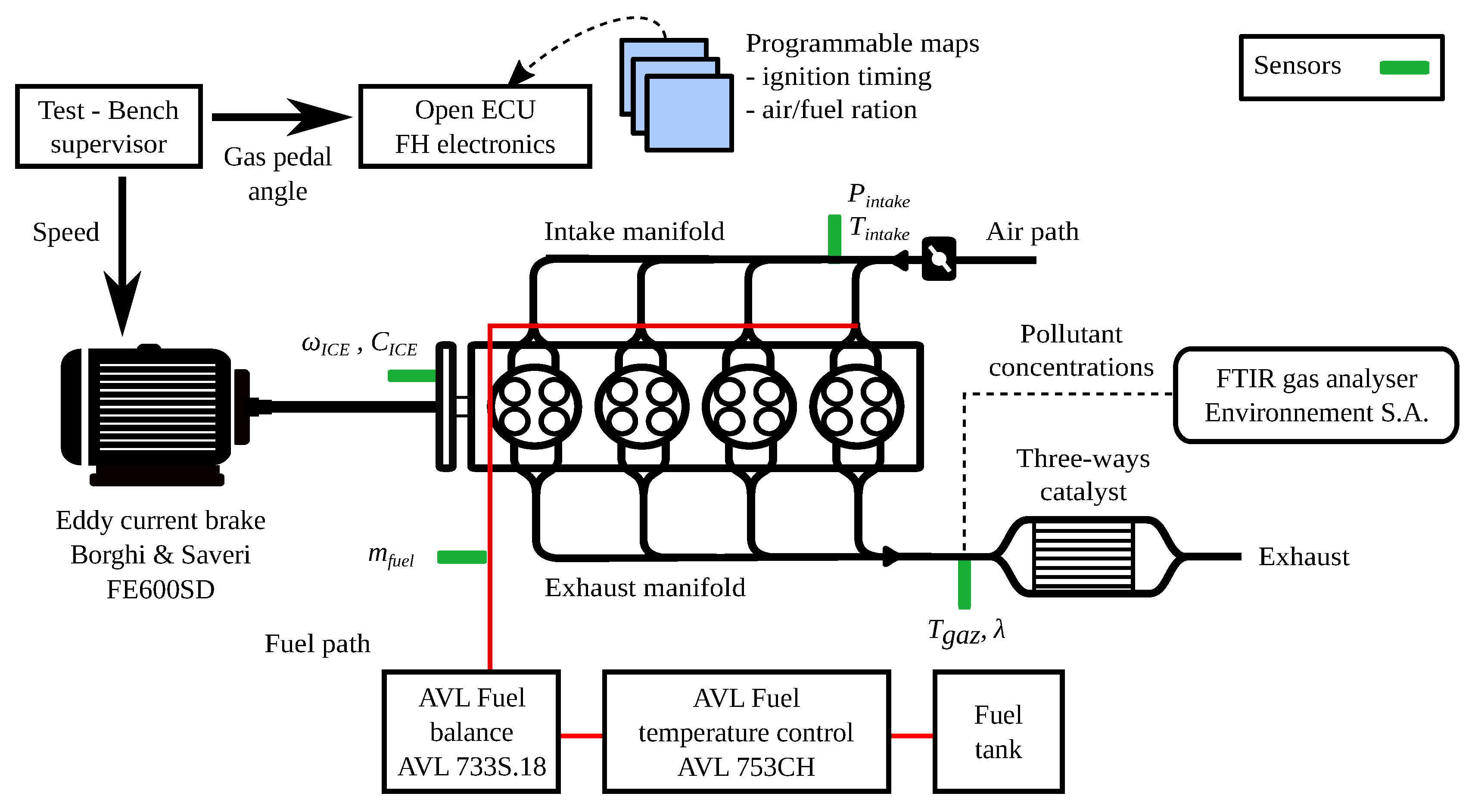
2.1. Experimental Setup and Procedure

The DRIVE laboratory’s test bench (see Figure 1) is equipped with the Renault D4F port fuel injection (PFI) engine (2000–2014). It allows measuring the exhaust gas temperature at the engine outlet with a type K thermocouple. A Fourier Transform Infrared spectrometer (FTIR) collects gas samples before the catalyst to measure the concentrations of carbon monoxide (CO), unburned hydrocarbons (HC) and nitric oxide (NO) at the engine outlet. A balance of consumption deduces the fuel mass flow rate used to feed the engine. The control parameters close to the engine (spark timing, air/fuel ratio of the mixture and the position of the throttle valve controlling the intake pressure) are adjustable by means of the open engine control unit (ECU).

The measurements were performed over a wide range of operating conditions as described in

Table 1. Operating conditions.

Intake manifold pressure (bar)	0.3    0.5    0.7    0.9    1
Engine speed (rpm)	800    1000    1500    2000    3000    4000
fuel/air eq. ratio (-)	0.7    0.8    0.85    0.9    0.95    1    1.1    1.2
Spark Advance (°BTDC)	−10: 5: 50

. The minimum spark advance value (i.e., spark retard compared to optimal which optimizes engine torque) corresponds to a temperature of 1000 K which should not be exceeded to avoid damage to the systems. The maximum value of spark advance is 25 degrees before the optimum advance. Depending on the chosen intake pressure (which determines the maximum pressure and temperature in the cylinder), some advances cannot be achieved because they may cause knocking. This phenomenon corresponds to a spontaneous-ignition of a part of the end-gas ahead of the flame. This ignition rapidly releases a large energy and causes high-frequency pressure oscillations which may damage the engine [5]. Almost 500 points were recorded in this campaign. Each operating point was stabilized during at least one minute before measuring. The data presented in this paper are available in the supplementary materials (see https://www.mdpi.com/2076-3417/11/3/971/s1).

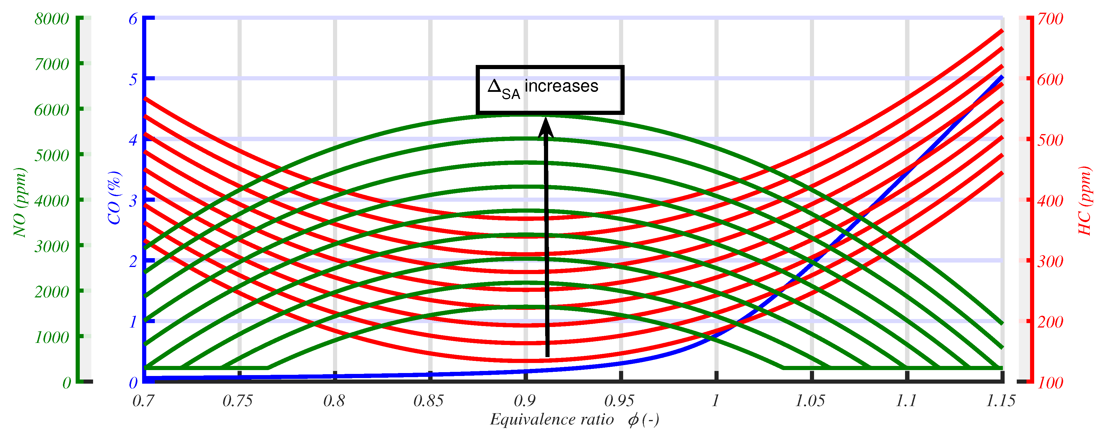
2.2. Emissions Model

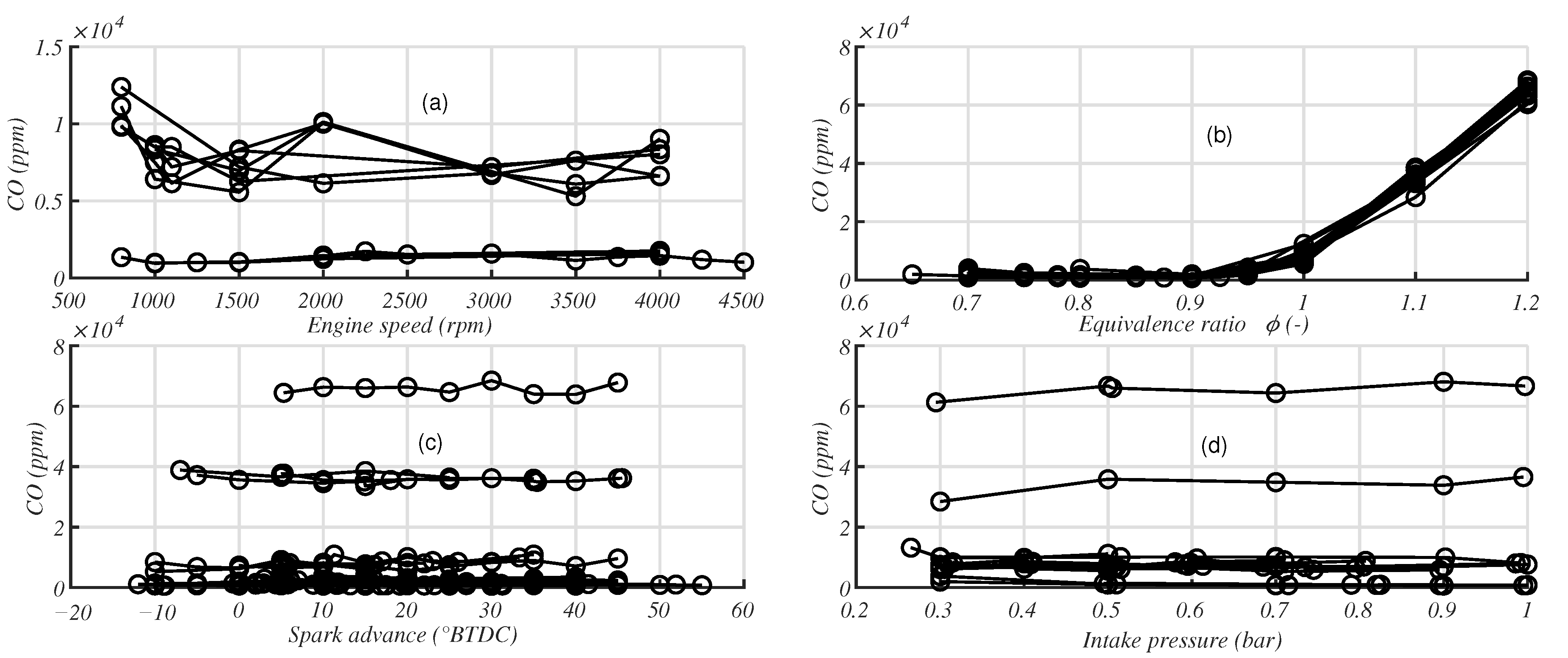
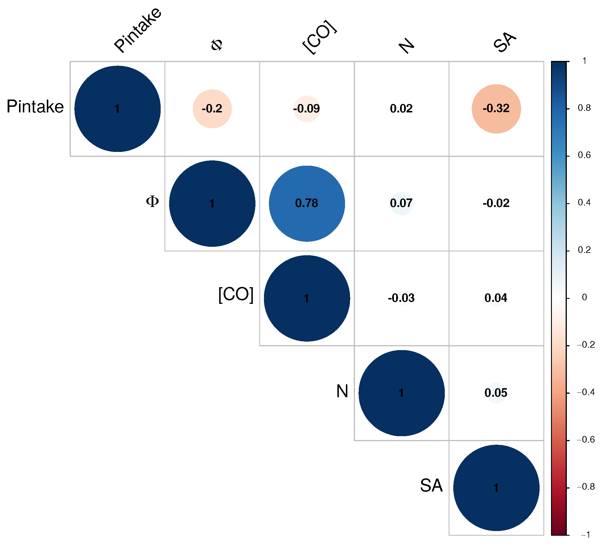
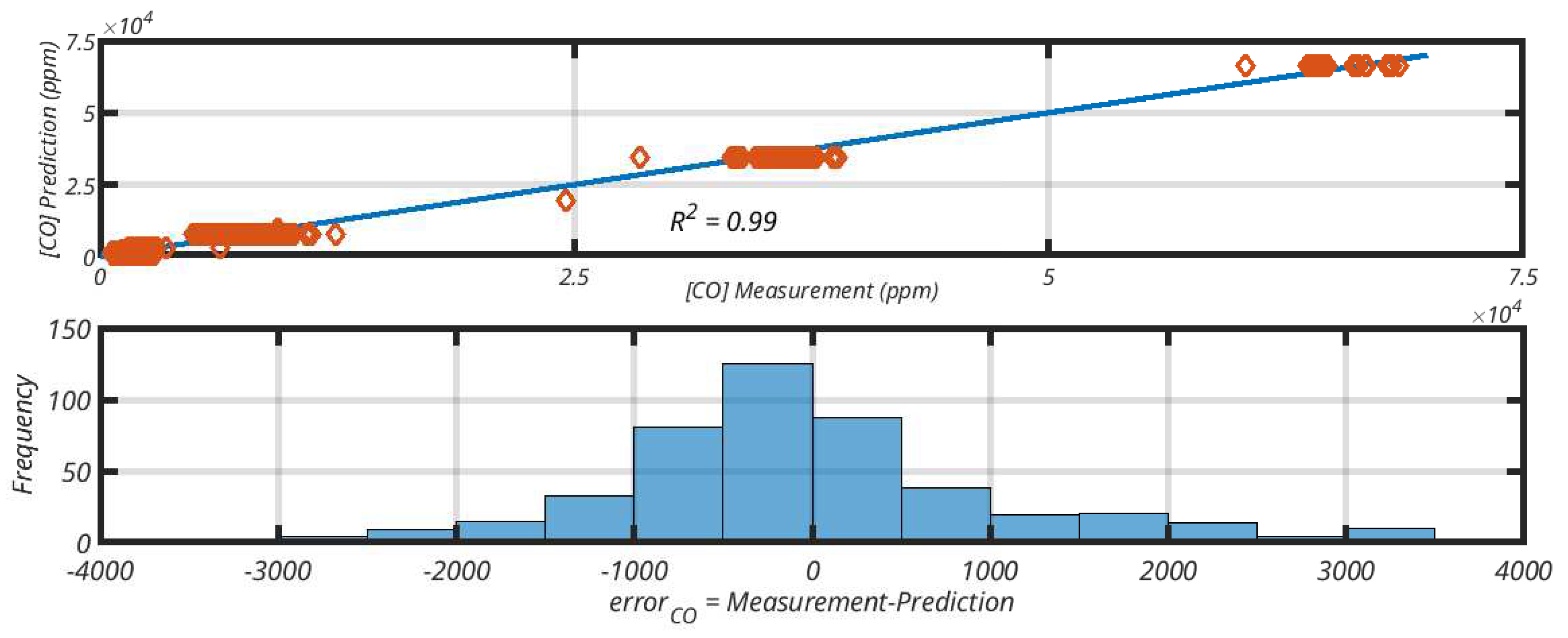
2.2.1. CO Model

Figure 2 is a graphical illustration of the measurements of CO concentration. Each graph represents the CO concentration as a function of one control parameter, i.e., (a) engine speed, (b) fuel/air equivalence ratio, (c) spark advance and (d) intake pressure. Each curve represents a series of measurements where only the parameter in abscissa changes.

The fuel is oxidized during combustion producing mainly CO, particularly abundant around the flame front [21]. This species is then itself oxidized in a second step to give carbon dioxide if the temperature and the quantity of oxygen are sufficient. Andrianov expresses CO concentration only as a function of the equivalence ratio that controls the amount of oxygen present in the cylinder [16]. This approach is consistent with the experimental results obtained as shown in Figure 2. Indeed, the curves representing the series where the speed, spark advance and pressure vary, are very close to horizontal straight lines. Whatever the value chosen for the variable on the abscissa, CO concentration is constant. Figure 3 is a correlogram between intake pressure, CO concentration, fuel/air ratio $\varphi$, engine speed N and Spark Advance SA. It allows analyzing the relationship between each pair of numeric variables in a dataset. We notice that neither spark advance, nor engine speed or intake pressure show high correlation factor with CO concentration. Andrianov [16] proposes to use a polynomial of degree 5 to model the dependence of the CO concentration on fuel/air ratio. Abida and Claude [13] use the root of a polynomial of degree 2, which gives a suitable shape by reducing the number of coefficients to be adjusted. We have therefore chosen to use the form proposed by Abida and Claude (Equation (1)) and to adjust the coefficients with the least squares method. In Equation (1), $\varphi$ represents the fuel/air equivalence ratio, $c{o}_1$ and $c{o}_2$ are the adjusting parameters. Symbols used in the document are described in the nomenclature section and values of the coefficients are listed in

Table A1. Parameters values for emission models.

${\mathbf{co}}_1$	164.073	${\mathbf{hc}}_1$	−0.0866	${\mathbf{no}}_1$	4.666
${\mathbf{co}}_{\mathbf{2}}$	0.00217	${\mathbf{hc}}_{\mathbf{2}}$	4976	${\mathbf{no}}_{\mathbf{2}}$	−73.687
		${\mathbf{hc}}_{\mathbf{3}}$	5.864	${\mathbf{no}}_{\mathbf{3}}$	105.7
		${\mathbf{hc}}_{\mathbf{4}}$	−0.1995	${\mathbf{no}}_{\mathbf{4}}$	−2669
		${\mathbf{hc}}_{\mathbf{5}}$	480.4	${\left[\mathbf{NO}\right]}_{\mathbf{min}}$	300

.

$$\left[CO\right]=c{o}_1\left(\varphi -1+\sqrt{{(\varphi -1)}^2+c{o}_2}\right)$$

(1)

Figure 4 shows that the proposed fit is in good agreement with the measurements. A large number of observations are concentrated around the origin of the graph which corresponds to low values of CO concentration. Indeed, a major part of the data have a fuel/air ratio lower than 1 (lean fuel mixture), so there is enough oxygen to convert CO into CO₂. The coefficient of determination is 0.99 and the mean error between the data and the predictions is 31%.

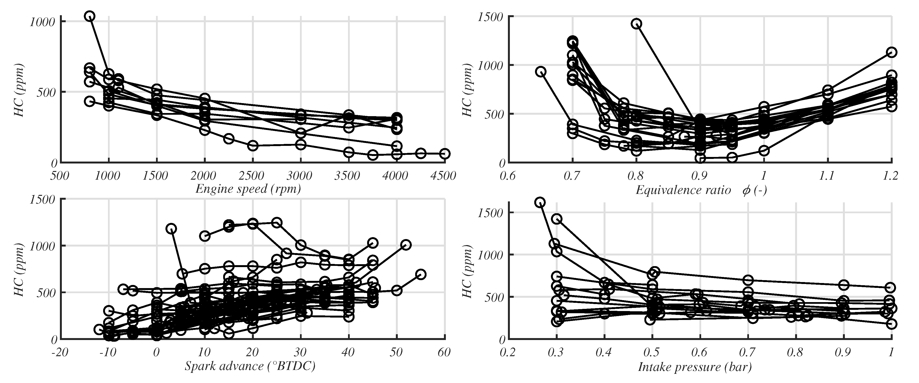
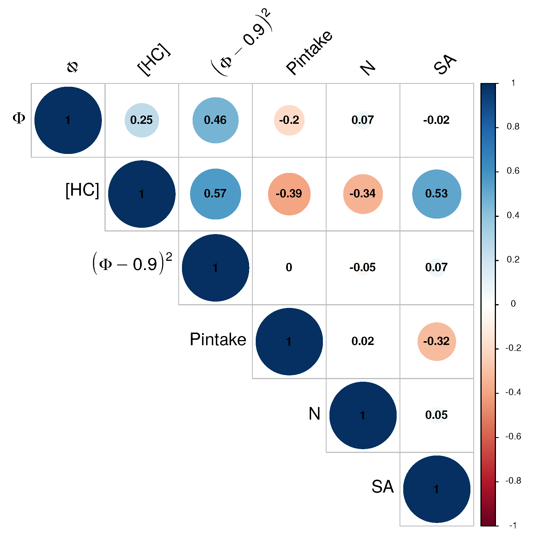
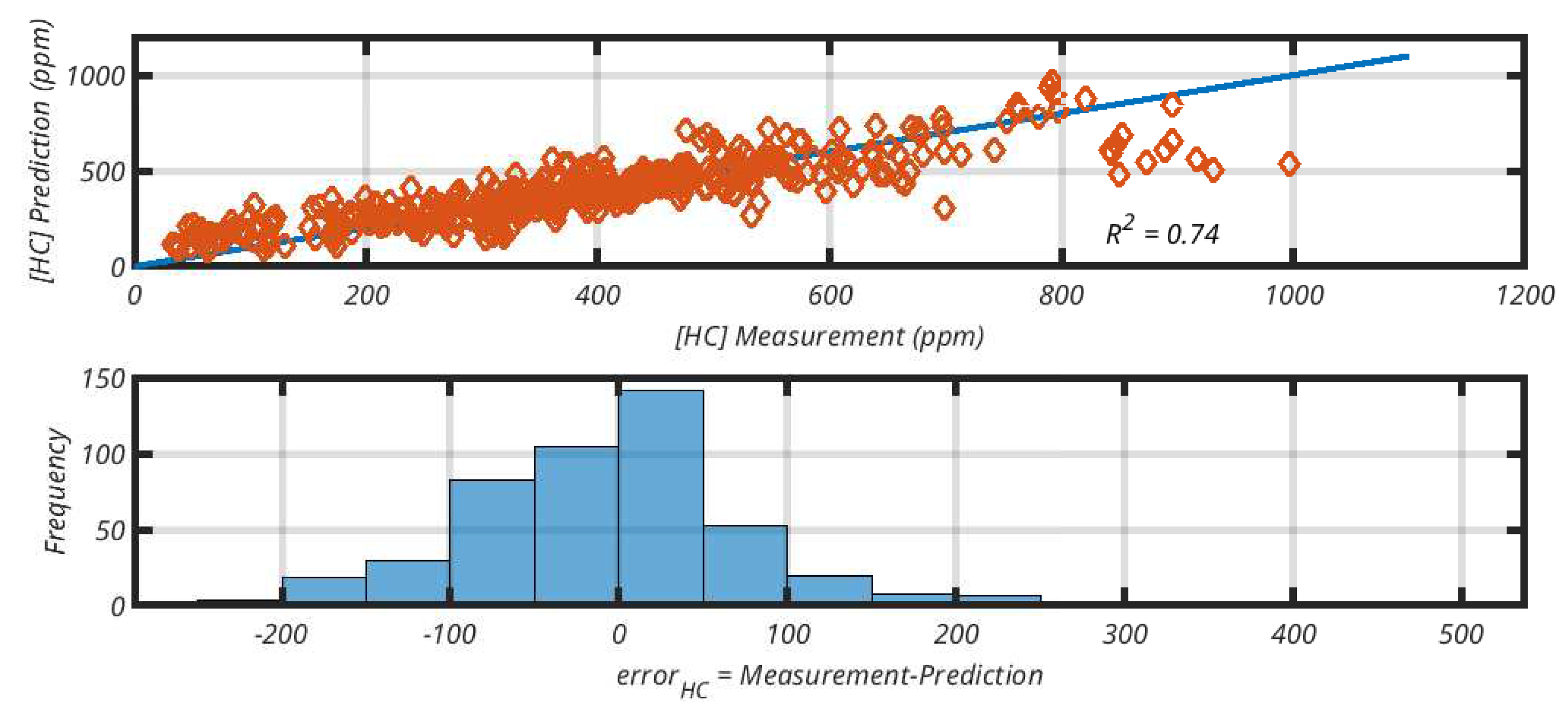
2.2.2. HC Model

Unburned hydrocarbons in gasoline engines mainly come from 4 mechanisms: flame quenching at the cylinder walls, entrapment of the unburned mixture in dead volumes (crevices), adsorption-desorption of the fuel in the oil film that covers the walls, and incomplete combustion or misfire [5].

Equivalence ratio has an influence on the emissions of unburned hydrocarbons. Indeed, if the mixture is very low in fuel, the flame speed is reduced which can lead to misfire and higher cyclic variability leading to significant increase in HC concentration. With a rich mixture, some of the fuel remains after combustion when all the oxygen has been used to produce carbon monoxide or dioxide and water. Furthermore, increasing $\varphi$ results in the raise of fuel vapor concentration in the bulk gas which will increase the absorption and hence the desorption from the oil layer [22]. Therefore the concentration of HC increases in both rich and lean mixes. This corresponds well to the behavior observed in Figure 5. Thus, we decided to introduce an augmented variable which is modeled by a second degree function around a minimum $\varphi$ value of 0.9.

The spark advance changes the HC emissions due to the storage of fresh gases in the crevices volumes and in the oil film on the walls [23]. This is because trapped hydrocarbons can be released and oxidized during the expansion phase if the temperature and amount of oxygen are sufficient. When the spark advance is high, combustion ends earlier, which does not allow efficient oxidation and increases HC concentrations. Figure 5 shows this behavior, which we have modeled by a linear function.

The speed has an influence on the internal aerodynamics of the engine. Increasing the speed improves the homogeneity of the mixture and promotes turbulence during combustion. The flame speed increases which improves combustion efficiency and reduces HC emissions [24]. Figure 5 shows this effect, which we modeled using a linear function.

When the mixture is lean, the fuel concentration is lower and the average free path of the molecules increases. On the other hand, when the intake pressure decreases, the fraction of residual gas in the cylinder increases which also contributes to dilute the fresh gas. Simultaneously, a decrease in the wall temperature is observed [22]. Low intake pressure can thus lead to incomplete combustion and increased HC emissions, especially in combination with lean burning. We have chosen to model this influence with a linear function.

As shown in Figure 6, HC emissions are positively correlated with Spark Advance SA and the augmented variable ${(\varphi -0.9)}^2$, and negatively correlated with intake pressure $P_{intake}$ and engine rotation speed N. The complete HC model expresses the causalities with the variables where $hc1$ to $hc4$ are the adjusting parameters. It is a linear model saturated to avoid negative concentrations that are not physically correct. Its expression is given by the Equation (2).

$$\left[HC\right]=max(0,h{c}_1·N+h{c}_2·{(\varphi -0.9)}^2+h{c}_3·SA+h{c}_4·P_{intake}+h{c}_5)$$

(2)

The values for the different parameters are listed in Table A1. Figure 7 shows that the proposed adjustment correlates with the observations. The coefficient of determination is 0.74 and the mean error between the measurements and the estimate is 27%. About ten points have measured HC emissions higher than 840 ppm and are slightly off-centre with respect to the fit line between the model and the data. These points correspond to low equivalence ratio ($\varphi <0.8$) and low or intermediate intake pressures ($P_{intake}\le 0.5$ bar) except for one point ($\varphi =0.65,P_{intake}=1$ bar).

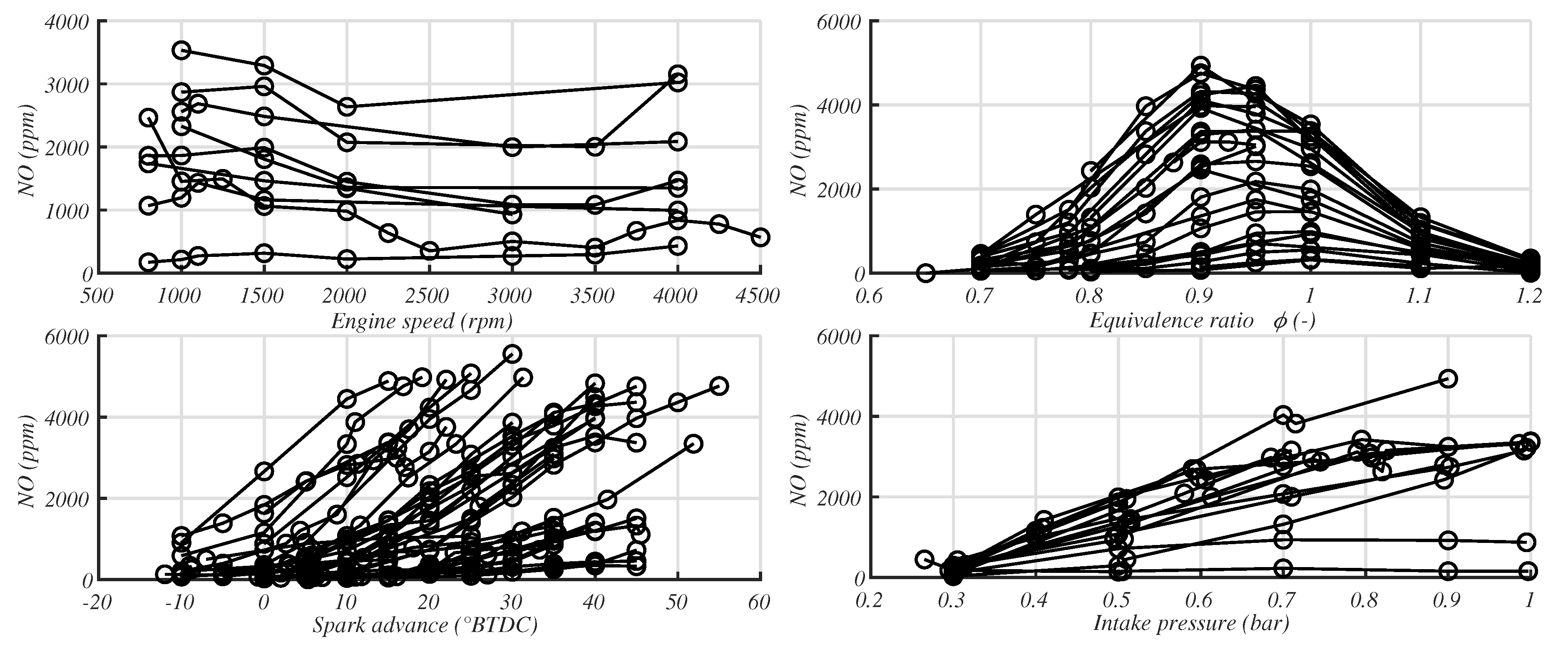
2.2.3. NO Model

The oxides of nitrogen $\mathrm{NO}$, ${\mathrm{N}}_2\mathrm{O}$ and ${\mathrm{NO}}_2$ are all present in the exhaust of a spark ignition engine. However, nitrous oxide is not significant as it represents less than 1% of $\mathrm{NO}$ emitted. Nitrogen dioxide can be more present with the maximum occuring at wide open throttle and a rich mixture. Nevertheless, its concentration is less than a few percent of $\mathrm{NO}$ [25]. This is confirmed by Bowman et al. [21], which states that: “$\mathrm{NO}$ is the predominant nitrogen oxide emitted by combustion devices”. In this context, the present work will focus on $\mathrm{NO}$ species. It can be produced by three distinct mechanisms:

• Early NO are formed at the flame front and in fuel-rich areas. They result from the combination of nitrogen N₂ with hydrocarbon radicals (C, C2, CH₂ or CH₂) to give the intermediate products HN, HCN, CN or CNH₂. These can recombine with oxygen to give nitrogen oxide NO [21].
• The NO-fuel are derived from the oxidation of the nitrogen atoms present in the fuel [26].
• Thermal NO is formed by the direct reaction of nitrogen and oxygen present in the air when the temperature and oxygen concentration are sufficient. This process is an important contributor to the total NO_x emissions and is known by the extended Zeldovich mechanism [5,9,27].

The rate of NO formation depends strongly on temperature as described by the Zeldovich mechanism. The temperatures necessary for NO formation are reached by the intense heat released during combustion (see Equation (3)).

$$\frac{d\left[NO\right]}{dt}=\frac{6·{10}^6}{\sqrt{T}}·exp\left(\frac{-69090}{T}\right)·{\left[O_2\right]}^{1/2}·\left[N_2\right]$$

(3)

The heat release varies depending on the mass of fuel injected. In gasoline engines, this is mainly controlled by the intake pressure, which regulates the amount of mixture introduced into the cylinder. Figure 8 shows that NO emissions increase with intake pressure. This behavior will be modeled by a linear function.

The spark advance also influences the maximum temperature reached during combustion. Indeed, the timing of the ignition with the compression phase of the gases by the piston influences the temperature and pressure at the beginning of combustion and during the propagation of the flame [28]. Higher pressure increases the volume concentration of the mixture and reduces the average free path of the molecules. Combustion is faster and the heat release is more intense, which increases the maximum combustion temperature and NO emissions. Figure 8 thus shows that NO emissions increase with spark advance. This influence will be expressed by a linear function.

Equivalence ratio $\varphi$ also plays an important role in the formation of NO. Under slightly lean fuel conditions ($0.9\le \varphi \le 0.95$), the fuel consumed allows the temperature of the cylinder to increase sufficiently and since oxygen is present in significant quantities, this favors the formation of nitrogen oxides. Leaner fuel conditions reduce the burned mass and therefore the maximum combustion temperature, which reduces NO emissions. Finally, a fuel-rich mixture reduces NO emissions because oxygen is consumed to produce CO or CO₂ via reactions that require less energy. The concentration of NO is therefore at a maximum and decreases in both rich and lean mixes. This corresponds well to the behavior observed in Figure 8 that we have modeled by a second degree function ${(\varphi -0.9)}^2$.

The correlogram (see Figure 9) also show a good correlation with ${(\varphi -0.9)}^2$. The engine speed does not have a strong influence on NO emissions as shown in Figure 8. We have therefore chosen not to include it in our model. Here again, we get a linear model with the augmented variable ${(\varphi -0.9)}^2$, where the four adjusting parameters are $n{o}_1$, $n{o}_2$, $n{o}_3$ and $n{o}_4$.

$$\left[NO\right]=max({\left[NO\right]}_{min},n{o}_1·{(\varphi -0.9)}^2+n{o}_2·SA+n{o}_3·P_{intake}+n{o}_4)$$

(4)

Figure 10 shows that the proposed adjustment corresponds well to the measurements with a coefficient of determination of 0.78.

To illustrate this part of our work, Figure 11 presents the concentration at ($N=2000$ rpm, $\varphi =0.9$ Bar) for various spark advance values.

2.3. Internal Combustion Engine Model

We need to make explicit the relationship between our control parameters and the engine model. This later comprises three parts: fuel consumption, brake torque and exhaust gas temperature. Fuel flow and torque models are mainly based on the literature, with forms inspired by those proposed by other authors. The temperature model rely on measurements made in the DRIVE laboratory with coefficients adjusted by the method of least squares.

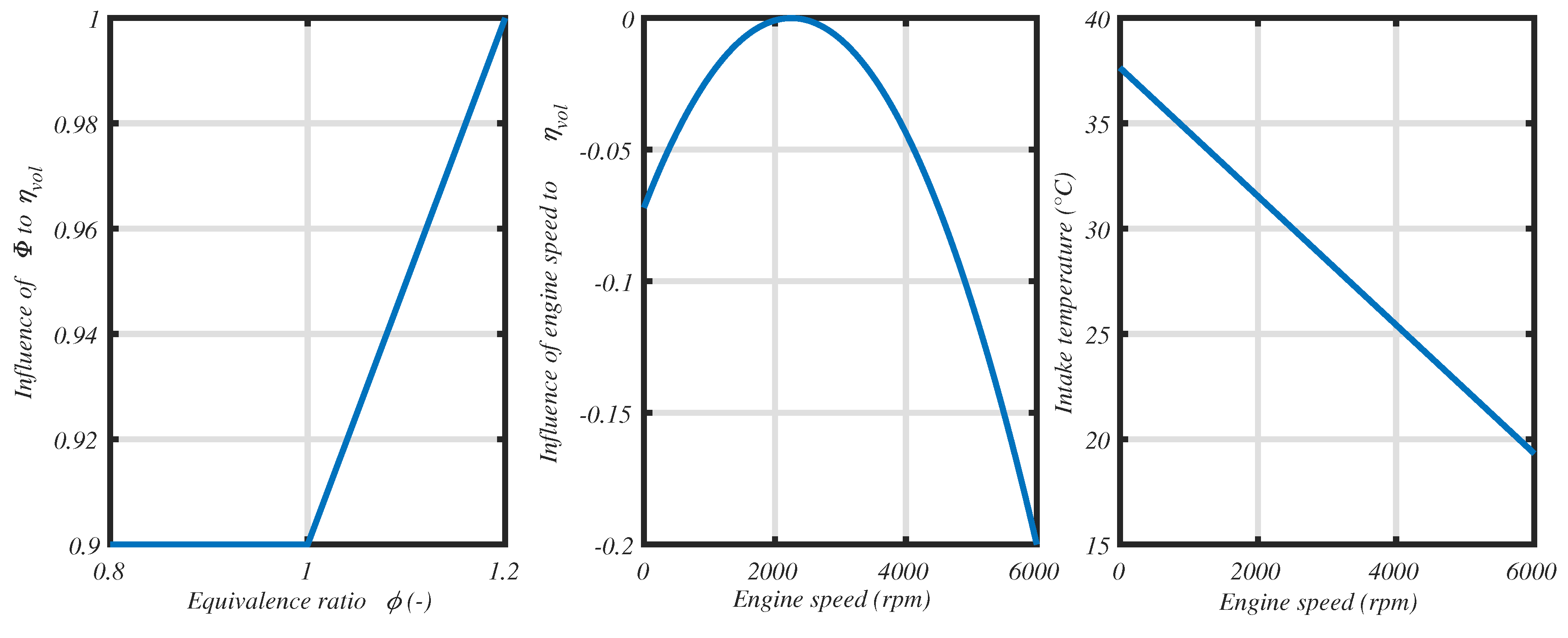
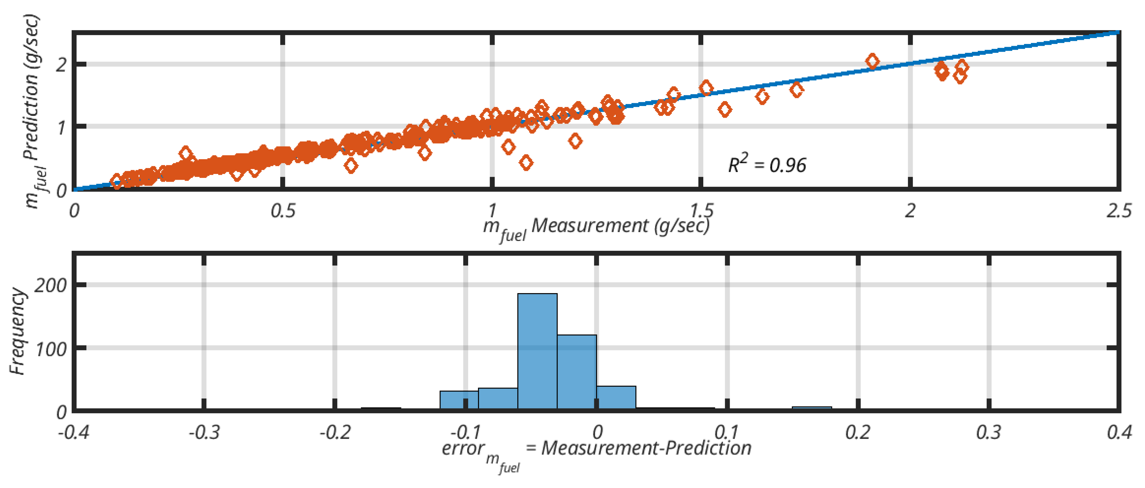
2.3.1. Fuel Flow

The air flow rate is proportional to the speed and intake pressure. The fuel flow rate ${\dot{m}}_{fuel}$ is itself proportional to the air flow rate, with the exception that it depends to the chemical composition of the mixture.

To increase the accuracy of the model, the volumetric efficiency ${\eta }_{vol}$ is introduced. It expresses the real efficiency of the engine compared to a perfect volumetric pump and therefore its capacity to introduce fresh gases (Equation (5)).

$${\dot{m}}_{fuel}=\frac{\varphi }{\varphi +{(m_{air}/m_{fuel})}_{st}}·{\eta }_{vol}·P_{intake}\times {10}^5·V_d·\frac{N}{60R_c}·\frac{M_{gaz}}{R_{gaz}·T_{adm}}$$

(5)

The fill rate is highly dependent on the speed that controls the gas flow rate at the inlet. The flow is limited by flow friction, especially around the valves, which increases with speed (and fluid velocity). Moreover, at very high speed, a critical flow rate is reached and limits the flow around the valve during at least part of the intake phase (chocking phenomenon) [29].

Conversely, filling at high speed can be improved by delaying the closing of the intake valve to take advantage of the inertia of the air column. This type of adjustment can result in intake backflow that degrades efficiency at low speed [5]. Finally, filling can be maximized for certain engine speeds thanks to an acoustic tuning that increases intake pressure by wave propagation phenomena [29].

The speed-dependent filling therefore has a maximum and decreases at both low and high speed. The position of the maximum depends on design choices and in particular on the geometry of the nozzles [27,30]. According to the studies, the filling rate evolves in a range of about 0.1 to 0.3 points and the corresponding maximum speed varies from 1250 to 4000 rpm [5,12,29,30].

We have chosen to model the effect of engine speed on fill rate by a quadratic function which has an amplitude of 0.2 points and a maximum for an engine speed of 2250 rpm (Equation (6) and Figure 12).

The filling rate is also influenced by the equivalence ratio of the mixture. This is because the fuel is injected as a liquid and vaporizes in the intake pipes. The heat consumed lowers the temperature and increases the density of the gases and the filling rate of the cylinder [5].

We chose to model this effect by varying the maximum value of the filling ratio (Equation (7) and Figure 12). This value is equal to 0.9 for a filling rate less than 1 (excess air) and increases for excess fuel (filling rate greater than 1).

$${\eta }_{vol}={\eta }_{vol,\varphi }-1.4\times {10}^{-8}·{(N-2250)}^2$$

(6)

$${\eta }_{vol,\varphi }=\left\{\begin{array}{cc}0.9\hfill & \varphi \le 1\hfill \\ 0.5·\varphi +0.4\hfill & 1<\varphi \le 1.2\hfill \end{array}\right.$$

(7)

Finally, the engine speed has an influence on the intake temperature [5]. Indeed, at low speed, the residence time of gases in the intake system is more important, which favors thermal exchanges with the hot walls and increases their temperature [31]. At high speed, the gases do not have time to warm up and remain at room temperature.

We have modeled this influence by a linear function of the speed, which has the largest temperature increase observed during the measurement campaign (16 °C) for the idle speed and decreases to room temperature for the maximum speed of 6000 rpm (Equation (8) and Figure 12).

$$T_{intake}=T_{amb}-0.003·N+18$$

(8)

We can see in Figure 13 that the model has a good fit to the measurements, with a determination coefficient of 0.96 and a mean error of less than 10%. Parameters values are listed in

Table A3. Parameters values for fuel flow, brake torque and exhaust temperature models.

${\mathit{R}}_{\mathit{c}}$	2	${\mathit{V}}_{\mathit{c}\mathit{y}\mathit{l}}$	1.8
${\eta }_{c0}$	0.98	${\eta }_{fi}$	0.43
A	300	$R_{gaz}$	8.314
B	2000	$LHV$	44,000
$a_{SA}$	5.507 · 10−5	${(m_{air}/m_{fuel})}_{st}$	14.7
$b_{SA}$	0.311	${\mathsf{\Delta }}_{SA,min}$	20
$C_{p,gaz}$	1.2 · 103	$a_N$	1.468 · 10−4
$a_{\varphi }$	−0.771	$b_N$	0.251
$b_{\varphi }$	1.503	$a_{Pintake}$	0.00108
		$b_{Pintake}$	0.805

.

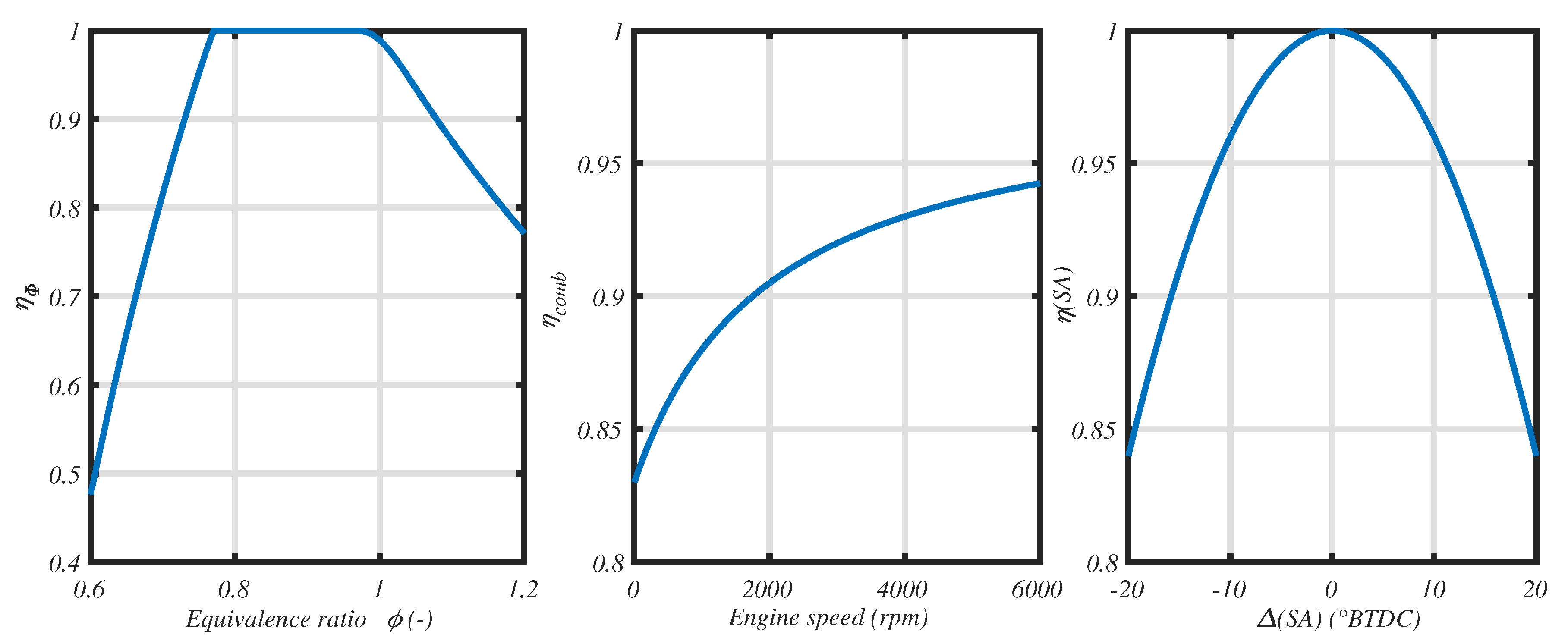
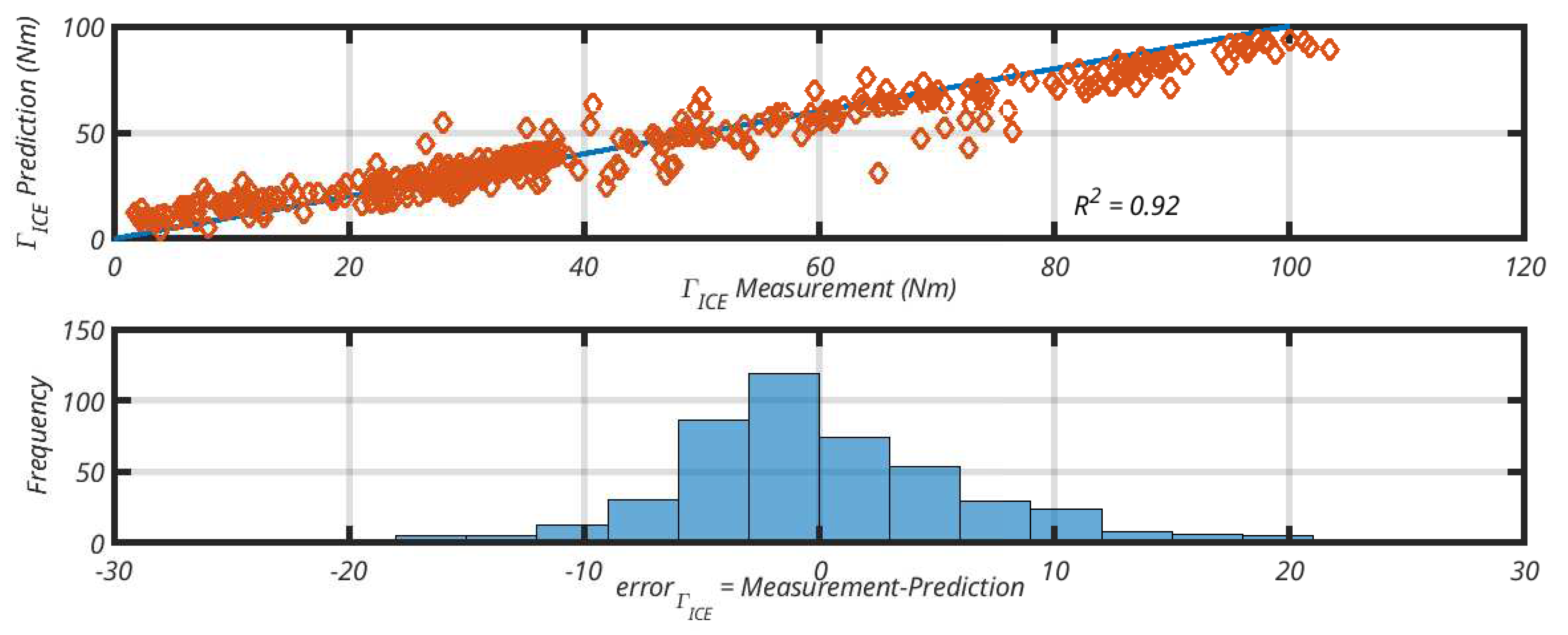
2.3.2. Brake Torque

By reversing the consumption model formulated by Asus et al. [19], we obtain a relationship between brake torque ${\mathsf{\Gamma }}_{ICE}$ and fuel flow ${\dot{m}}_{fuel}$ (Equation (9)). In this expression, brake torque is proportional to the ratio between flow rate and engine speed N, with an extra term that estimates friction torque. The coefficient of proportionality corresponds to the engine efficiency, which depends on the parameters of close control of the engine (speed, equivalence ratio and spark advance), based on the shapes proposed by Guzzella and Onder [12].

The evolution of combustion efficiency with speed is taken from the model proposed by Asus et al. [19] (Equation (10) and Figure 14). The shape of the friction torque ${\mathsf{\Gamma }}_f$ is based on a Heywood model [5] (Equation (11)).

$${\mathsf{\Gamma }}_{ICE}={\eta }_{fi}·{\eta }_{comb}·{\eta }_{\varphi }·{\eta }_{SA}·\frac{{\dot{m}}_{fuel}·LHV}{\pi N/30}-{\mathsf{\Gamma }}_f$$

(9)

$${\eta }_{comb}=\left({\eta }_{c0}-\frac{A}{B+N}\right)$$

(10)

$${\mathsf{\Gamma }}_f=(97+0.015·N+5\times {10}^{-6}·N^2)·\frac{V_d}{2\pi R_c}$$

(11)

Efficiency as a function of equivalence ratio decreases when the mixture is rich. This is because the extra fuel is not converted into energy due to a lack of oxygen. In addition, oxygen depletion can lead to incomplete combustion and reduce thermodynamic efficiency. On the contrary, in a lean mixture, all the fuel introduced can be consumed and the efficiency keeps a value of 1 over a wide range [12].

The model of Guzzella and Onder takes into account these two phenomena. They thus propose a curve proportional to the excess air, a transition then a step at 1. However, it is only applicable for equivalence ratio greater than 0.77. For fuel contents below this limit, combustion misfires may occur due to the low fuel concentration [12]. Performance deteriorates thus quickly until combustion becomes impossible (lean flammability limit) [32]. We have chosen to model this behavior by a portion proportional to the excess air with a slightly larger directing coefficient than that of the rich mixture. The complete model is given by Equation (12) and plotted in Figure 14.

$${\eta }_{\varphi }=\left\{\begin{array}{cc}1.373/\varphi -0.373\hfill & 0.7\le 1/\varphi <0.95\hfill \\ 0.9313+(1-0.9313)·sin\left(\frac{1/\varphi -0.95}{1-0.95}\right)\hfill & 0.95\le 1/\varphi <0.95+\frac{\pi }{2}(1-0.95)\hfill \\ 1\hfill & 0.95+\frac{\pi }{2}(1-0.95)\le 1/\varphi <1.3\hfill \\ -1.4286/\varphi +2.8571\hfill & 1.3\le 1/\varphi <1.54\hfill \end{array}\right.$$

(12)

Spark advance has a significant impact on the conversion of thermal energy into mechanical energy. For a given speed, fuel/air ratio and fuel flow, there is an optimal advance that maximizes the torque and thus the engine’s efficiency [5,12,33].

A relative spark advance (symbol $\mathsf{\Delta }SA$) can therefore be defined, which is the difference between the selected setting and the optimum spark advance for a given operating point. For the D4F engine used for this study, the optimal spark advance as a function of engine speed and intake pressure was determined during previous test campaigns (optimal values are reported in

Table A2. Optimal values for spark advance as a function of intake pressure and engine speed.

		N (rpm)
		500	750	1000	1500	2000	2500	3000	3500	3750	4000	4500	5000	5500	6000
${\mathbf{P}}_{\mathbf{intake}}$ (mBar)	200	29	30	33	36	38	40	40	40	44.1	40	40	40	40	40
	300	30	30	30	33	36	40.1	40.1	38,1	42.1	40.1	40	40	40	40
	400	28	28	30	32	33.3	35.1	35.1	34.1	34.1	34.1	34	34	34	34
	500	22	25	28	30	31.1	33.1	31.1	29.1	32.1	31.1	31	31	31	31
	600	20	23	25	27	28.1	29.1	28.1	27.1	29.1	30.1	29	29	29	29
	700	19	20	20	21	23.1	27.1	28.1	26.1	26.1	26.1	26	26	26	26
	800	21	20	20	24	21.1	26.1	28.1	24.1	25.1	24.1	25	25	25	25
	900	20	22	20	22	21.1	24.1	24.1	24.1	24.1	24.1	24	24	24	24
	1000	20	20	20	17	19.1	21.1	21.1	20.1	23.1	24.1	21	21	21	29

). We thus determine the relative advance for the various measurements carried out on the bench using the table of optimal advances (according to Equation (14)). The shape of the efficiency with regards to relative advance is inspired by Guzzella and Onder [12] (Equation (13) et Figure 14).

$${\eta }_{SA}=1-0.04\times {10}^{-2}·{\mathsf{\Delta }SA}^2$$

(13)

$${\mathsf{\Delta }}_{SA}=SA-S{A}_{opti}(N,P_{intake})$$

(14)

We notice from Equation (14) that a negative value of ${\mathsf{\Delta }}_{SA}$ brings the ignition closer to top dead center, and a positive value of ${\mathsf{\Delta }}_{SA}$ increases the spark advance.

We can see in Figure 15 that the model has a good fit to the measurements, with a determination coefficient of 0.92 and a mean error of 30%.

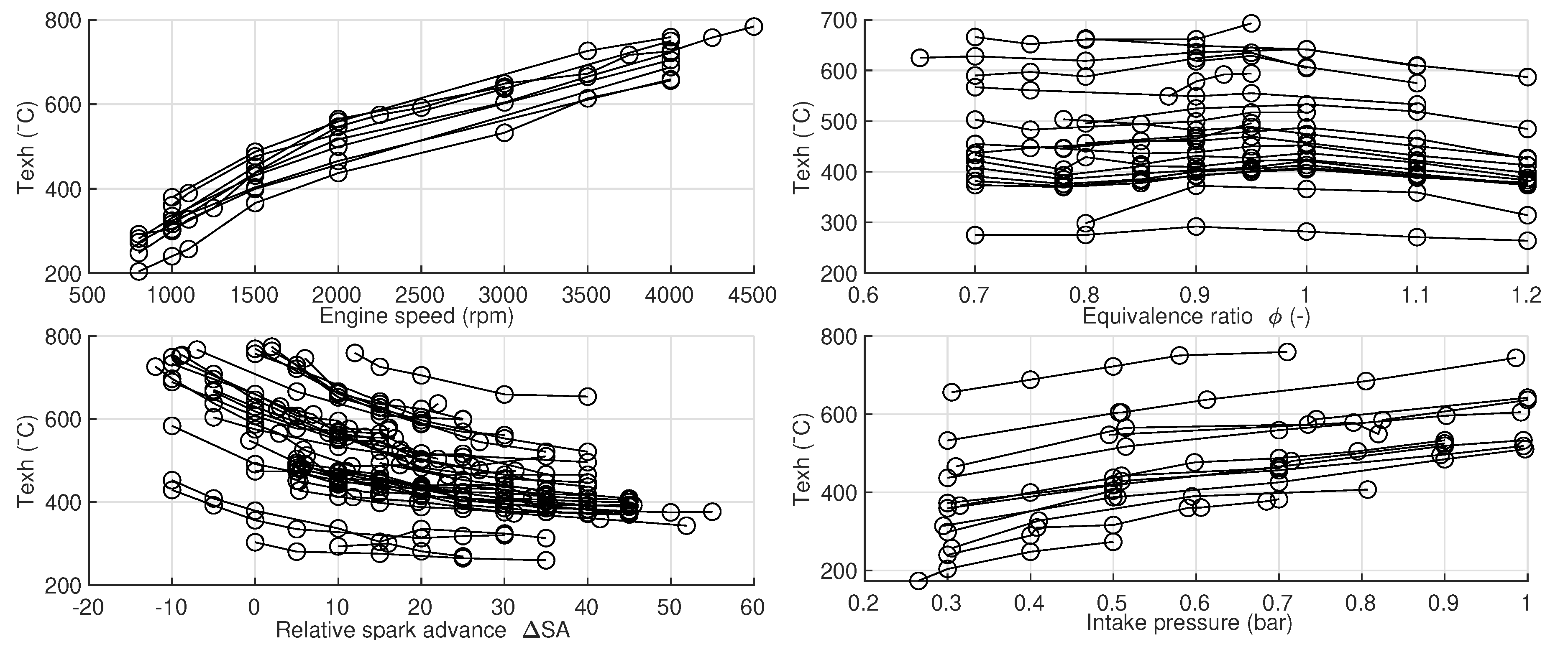
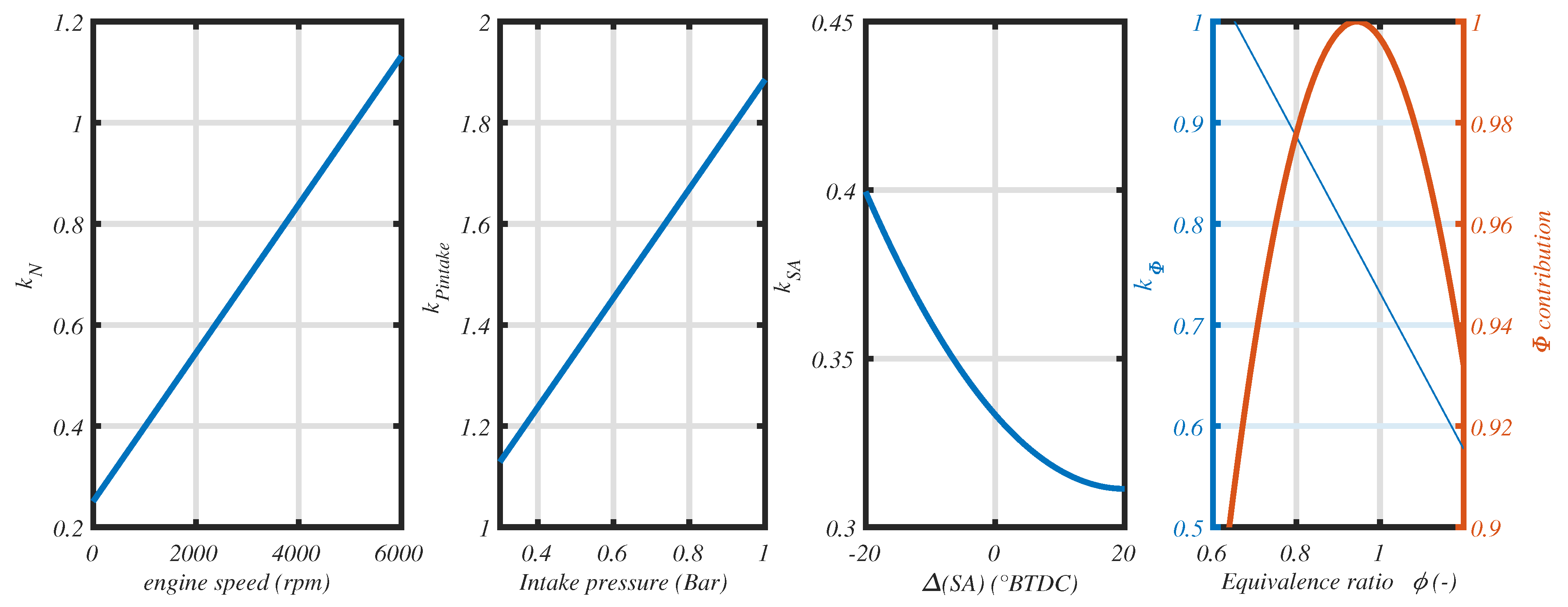
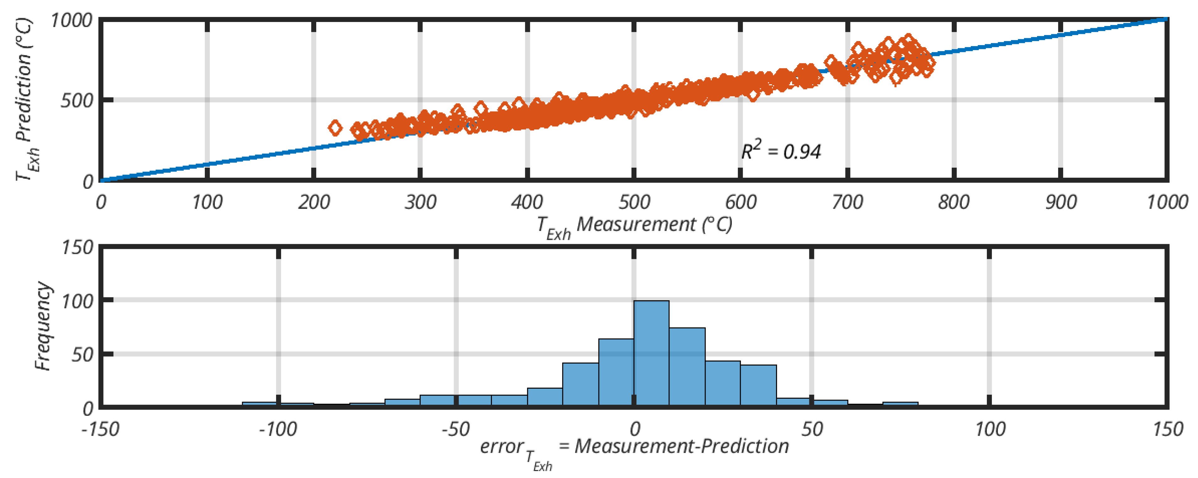
2.3.3. Exhaust Temperature

Last but not least exhaust temperature model has to be defined with regards to its action on catalytic converter behavior. Figure 16 represents the measurements. In the bottom left graphic, the exhaust temperature is described versus the relative spark advance. It should be noted that this was not the case for emissions plots presented above.

The temperature rise at the engine outlet depends on the proportion of energy involved in combustion that remains in the exhaust and the thermal capacity of the gases. The proportion of energy still present in the exhaust depends on the engine’s close control parameters. The exhaust temperature depends on the temperature rise and the intake temperature (Equation (15)). The latter is calculated using the same formula as for the flow model (Equation (8)).

$$T_{exh}=T_{intake}+\frac{k_{\varphi }·k_{SA}·k_N·k_{Pintake}·LHV}{C_{p,gaz}·(1+\frac{{(m_{air}/m_{fuel})}_{st}}{\varphi })}$$

(15)

Engine speed and intake pressure control the flow of gases into the engine. The higher the flow rate, the less time available for heat exchange with the walls relative to the quantities involved [5,12]. Heat losses at the walls decrease and the exhaust temperature increases. This behavior is apparent in Figure 16, and we have chosen to model the influence of these parameters with two linear functions (Equations (16) and (17)).

$$k_N=a_N+b_N·N$$

(16)

$$k_{Pintake}=a_{Pintake}+b_{Pintake}·P_{intake}$$

(17)

The influence of equivalence ratio on exhaust temperature is similar to its effect on maximum combustion temperature (see Section 2.2.3) [5]. Both excess fuel and excess air form an inert mass that lowers the temperature in the cylinder and at the exhaust. The latter has therefore a maximum around the stoichiometric air/fuel ratio as shown in Figure 16. As the temperature model already depends on the equivalence ratio by the multiplicative factor in the denominator, we have added a linear function of the equivalence ratio to the numerator (Equation (18)) which allows obtaiingn a parabolic shape for the global influence of this parameter.

$$k_{\varphi }=a_{\varphi }+b_{\varphi }·\varphi$$

(18)

Finally, the later the ignition occurs (negative relative spark advance, i.e., spark retard), the more the combustion shifts towards the opening of the exhaust valve and the more the temperature increases, as shown in Figure 16. We have chosen to model this effect with a parabola (Equation (19)).

$$k_{SA}=a_{SA}+b_{SA}·{({\mathsf{\Delta }}_{SA}-{\mathsf{\Delta }}_{SA,min})}^2$$

(19)

The 9 model fitting parameters were determined using the method of least squares (2 constants for speed, pressure and fuel/air ratio, and 3 for spark advance). The Figure 17 shows the shapes of the coefficients which express the portion of residual energy at the exhaust. The global contribution of the wealth (in orange) corresponds to the (scaled) ratio between $k_{\varphi }$ and the coefficient depending on $\varphi$ in the denominator. The model corresponds well to the measurements as can be seen in Figure 18, with a determination coefficient of 0.94 and a mean error of 5.6%.

2.4. Catalyst Model

The catalytic converter used in this study conforms to the EURO 6 emission standard. It is light and closely coupled to the engine for an accelerated light-off. The model (that is efficiency as a function of temperature and equivalence ratio, thermal behavior) has been widely described in reference [20] and the reader can refer to this article for further informations. Figure 19 shows the thermal validation on the WLTC (Worldwide harmonized light-duty vehicles test cycle).

2.5. Vehicle Dynamics

Vehicle dynamics and resulting power demand are modeled using a backward approach. The velocity as a function of time is known in advance and this driving cycle corresponds to a necessary torque at the wheels (${\mathsf{\Gamma }}_{wheel}$) to overcome the inertia of the vehicle as well as the resistive forces acting on it. The mechanical transmission components have constant efficiencies and the engine speed is saturated to its idle speed to model the clutch behavior.

$${\mathsf{\Gamma }}_{wheel}=F_{res}{R}_{tire}+\frac{J_{veh}}{R_{tire}}\frac{dv}{dt}$$

(20)

$$F_{res}=m_{veh}g{k}_{rol}+\frac{1}{2}\rho S_F{C}_x{v}^2$$

(21)

$$J_{veh}=m_{veh}{R}_{tire}^2+4J_{wheel}$$

(22)

$${\mathsf{\Gamma }}_{ICE}={\mathsf{\Gamma }}_{wheel}\frac{{\eta }_{DF}^e{\eta }_{GB}^e}{k_{DF}{k}_{BV}}+J_{ICE}{\dot{\omega }}_{ICE}$$

(23)

$$e=\left\{\begin{array}{cc}-1\hfill & {\mathsf{\Gamma }}_{wheel}>0\left(\mathrm{traction}\right)\hfill \\ 1\hfill & {\mathsf{\Gamma }}_{wheel}<0\left(\mathrm{brake}\right)\hfill \end{array}\right.$$

(24)

$${\omega }_{ICE}=max\left({\omega }_{idle},\frac{v}{R_{tire}}{k}_{DF}{k}_{GB}\right)$$

(25)

2.6. Problem Formulation and Discretization Values

Dynamic programming is based on Bellman’s principle of optimality. State variables are discretized temporally and on a scale of values. A graph whose vertices are defined by the value taken by the state variable at a given instant is thus constructed. The path from one vertex to another is associated with a value of the command and a cost from the point of view of the objective function. The path that minimizes the sum of the costs in the graph corresponds to the sequence of the optimal values of the command.

The associated optimal control problem is given by Equation (26), which is the weighted sum of pollutant emissions and fuel consumption.

$$J=\sum _{cycle}\left(\frac{{\dot{m}}_{fuel}}{{\dot{m}}_{fuel,ref}}\delta t+\frac{\alpha }{3}\left(\frac{{\dot{m}}_{CO}}{{\dot{m}}_{CO,ref}}+\frac{{\dot{m}}_{HC}}{{\dot{m}}_{HC,ref}}+\frac{{\dot{m}}_{NO}}{{\dot{m}}_{NO,ref}}\right)\delta t\right)$$

(26)

Both fuel consumption and pollutant emissions show extremely different orders of magnitude. To normalize them we consider the simulation of the reference vehicle for which mixture is stoichiometric and spark advance is optimal.

There are three control variables in the optimal control problem, intake pressure, relative spark advance and fuel/air equivalence ratio. By mixing Equations (5) and (9), we calculate the necessary intake pressure that satisfies Equation (23) and the required engine torque at each time step, thus reducing the problem complexity with two control variables only.

The state variable is the catalyst temperature as it drives the catalyst overall efficiency and the associated emitted pollutants. The problem is subject to its first-order dynamics expressed in discrete form. It can vary freely during the driving cycle, its initial temperature is ambient temperature and its final value is unconstrained.

The catalyst monolith temperature varies continuously despite the discrete control variables. To obtain a temperature mesh, it is rounded as expressed by Equation (27). The impact of the mesh precision will be discussed in the following section.

$$\mathsf{\Delta }{T}_{cata}=\mathrm{round}\left(\frac{\delta t}{m_{cata}{C}_p}({\dot{Q}}_{amb}+{\dot{Q}}_{gaz}+{\dot{Q}}_{reac})·\frac{1}{\delta T}\right)\delta T$$

(27)

Table 2. Discretization step size used in this paper.

Variable	Steps	Min. Value	Max. Value
catalyst temperature	0.1 K	not bounded
Fuel/air eq. ratio	0.01	0.7	1.1
Relative spark advance	2°	−30°	10°
Step time	1 s	NA

summarizes the discretization steps for the state and the control parameters.

3. Results

The reference vehicle used in the present study is a conventional one whose characteristics are given in

Table 3. Main vehicle characteristics and types of model used in this study.

Component	Size	Type of Model
Internal combustion engine	1.8 L	Mean Value Engine Model
Three way catalytic converter	EURO 6 compliant	0D model
Chassis (Peugeot 308 SW-2009)	1470 kg	longitudinal forces

. The numerical parameters are given in

Table A4. Parameters value for the vehicle model.

${\mathit{\eta }}_{\mathit{D}\mathit{F}}$	0.97	${\mathit{k}}_{\mathit{r}\mathit{o}\mathit{l}}$	0.008
${\eta }_{GB}$	0.95	$S_F$	0.728
$\rho$	1.1841
$k_{DF}$	4.7647	$C_x$	1
$k_{GB}$	[3.4545 1.8667 1.2903 0.9512 0.7447]	$m_{veh}$	1499.3
$J_{wheel}$	0.7
$R_{wheel}$	0.3069	${\omega }_{idle}$	78.53

. Figure 20 represents the vehicle speed and gearbox ratio during the NEDC cycle that was used to obtain the first results. The value of the weighting factor $\alpha$ between pollutant emissions and fuel consumption allows the definition of several scenarios. In the first part of this section, we present a pollution centered scenario which is compared to the reference strategy where nominal parameters are retrieved (i.e., equivalence ratio equals to 1 and optimal spark advance).

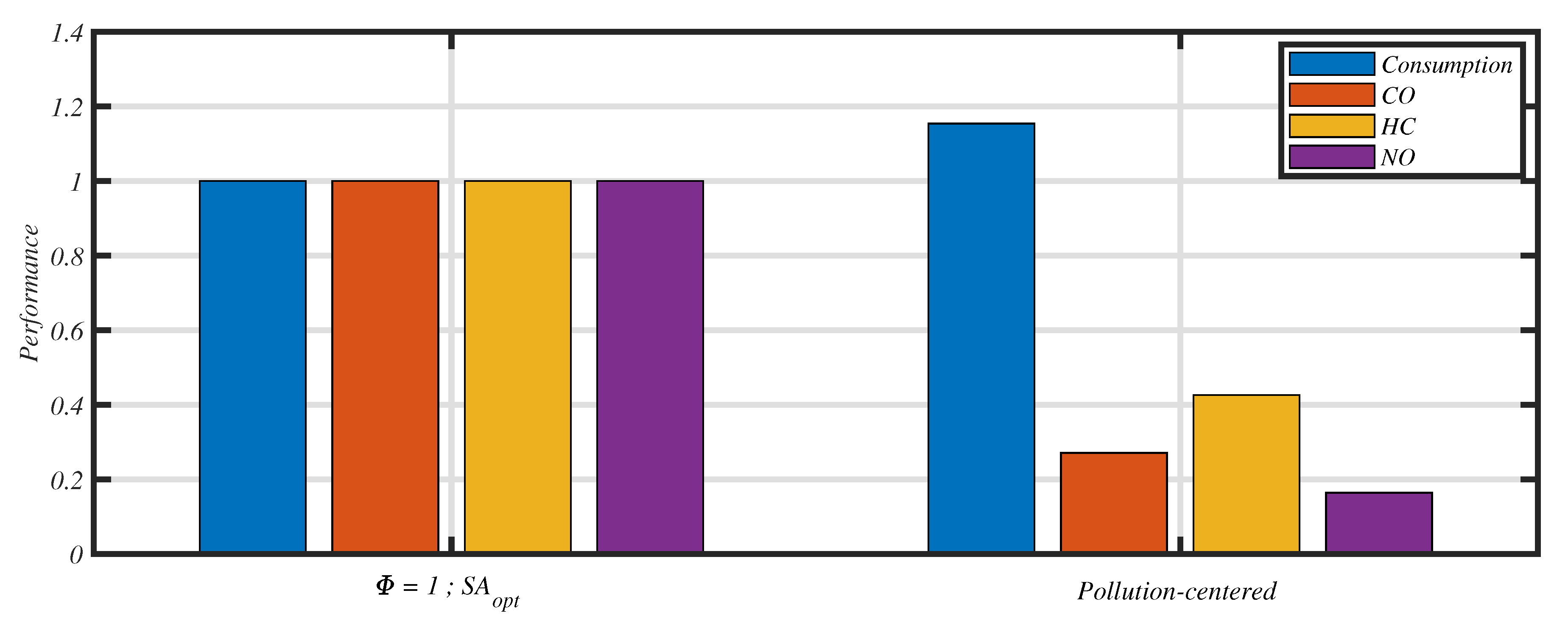
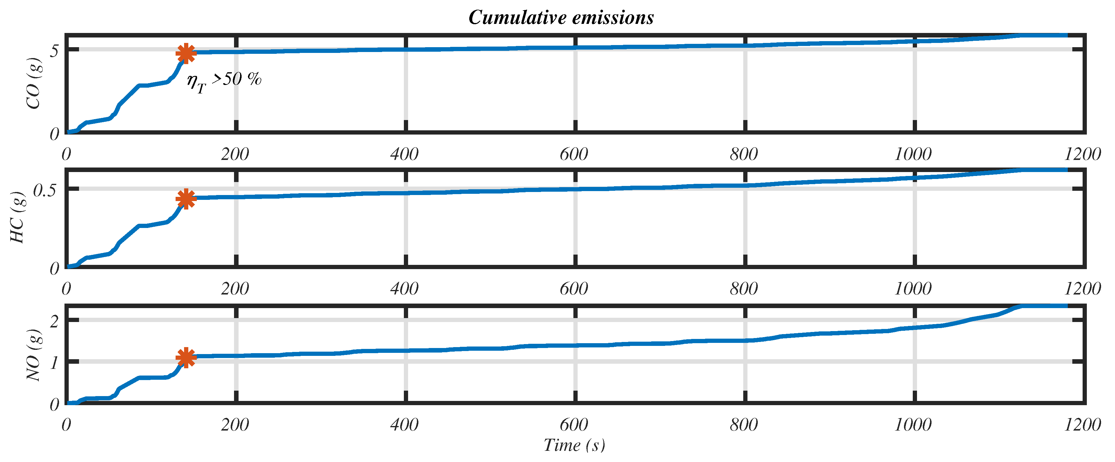
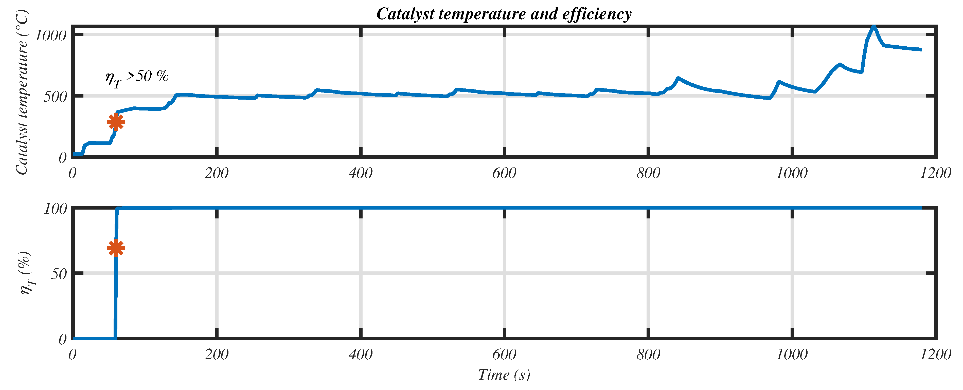
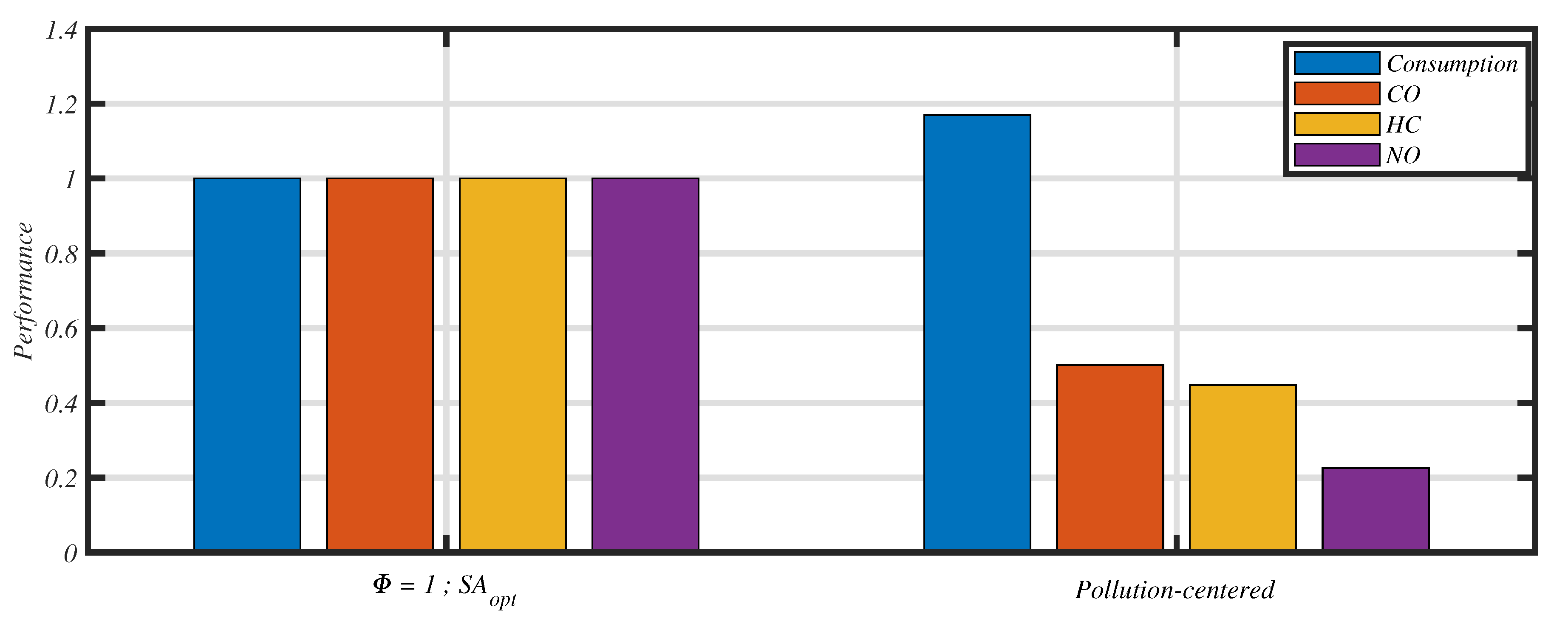
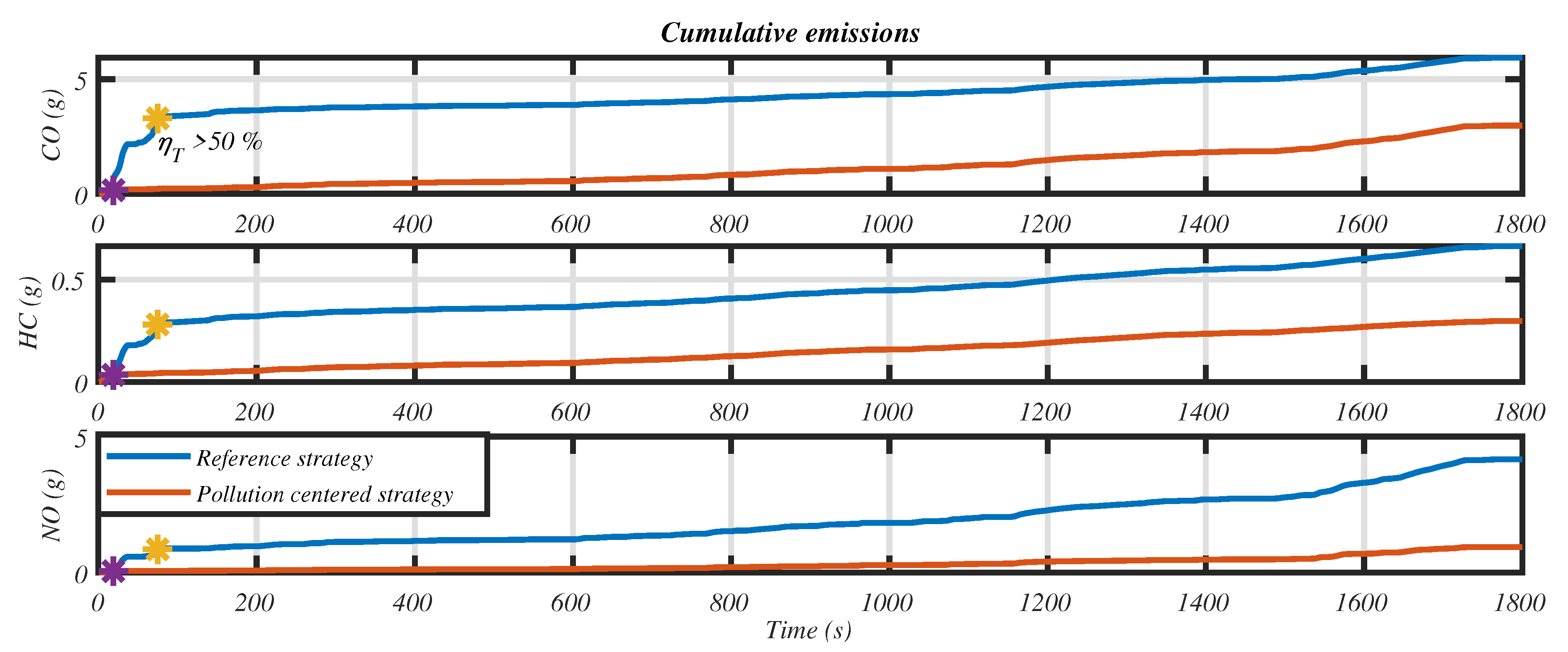
3.1. Pollution Centered Scenario

One can see the performance of the pollution centered scenario in Figure 21 (in this case, the weighting parameter, $\alpha$, is equal to 5) compared to the reference strategy. Fuel consumption increases by 15%, but we observe a great reduction in pollutant emissions: 73% for CO, 57% for HC and 84% for NO. Numerical results are presented in

Table 4. Performance of the pollution centered scenarios compared to the reference strategy (NEDC).

	Ref. Strategy ${\mathit{SA}}_{\mathit{opti}}$ $\mathit{\varphi }=1.0$	$\mathit{\alpha }=5$ $\mathit{SA}\mathit{var}$ $\mathit{\varphi }\mathit{var}$	Relative Variation
Consumption (L/100 km)	6.57	7.59	+15%
CO (g/km)	0.53	0.144	−73%
HC (g/km)	0.056	0.024	−57%
NO (g/km)	0.212	0.035	−84%

.

As it can be seen in Figure 22 and Figure 23, the catalyst light-off (instant where catalyst efficiency reaches 50% which corresponds to a temperature of 280 °C) is reached at 140 s. At this time, more than 80% of total CO have already been emitted, while almost 70% of total HC are produced. 50% of total tailpipe NO have already been dispersed in the environment.

The behavior of the engine is far different with the pollution centered scenario (see Figure 24): the light-off of the catalyst is quicker, as it happens after only 60 s. Furthermore, a very small amount of pollutant is emitted during this period as illustrated in Figure 25: CO are reduced by a factor of 15, HC by 4, and NO_x emissions before light-off are 11 times lower than in the nominal configuration.

Figure 26 shows the positions of the actuators during the pollution centered scenario: We can distinguish between two different behaviors:

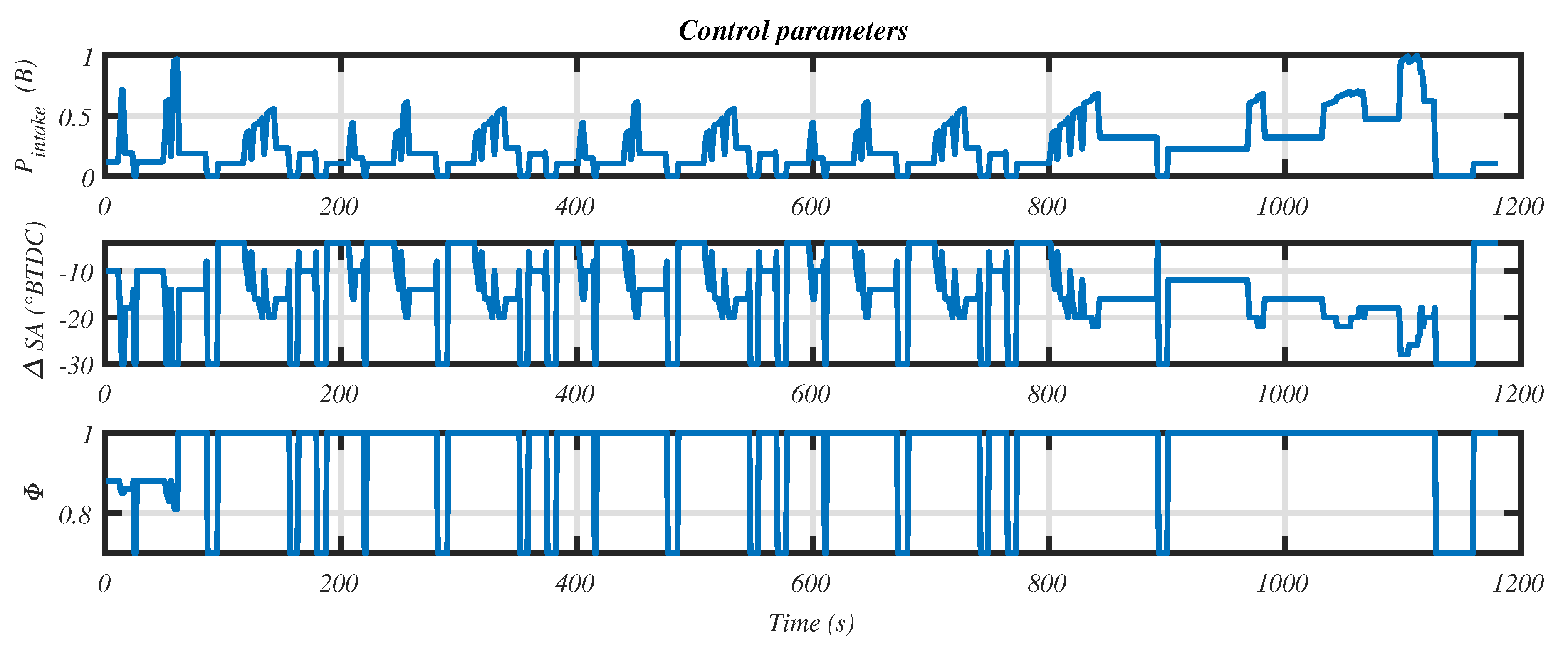
• Catalyst light-off: during this period, we observe a late spark advance (10 to 15° compared to optimal ignition). This is combined with a lean mixture, $\mathsf{\Phi }=0.9$. These two parameters increase the exhaust gas temperature. For constant engine torque, the reduced fuel conversion efficiency associated with late combustion requires greater fuel and air flow rate (see intake pressure in Figure 26). As a consequence, exhaust enthalpy and convective effects are high. This shortens the period where catalyst efficiency is low.
• warm catalyst period: the strategy adopts a stoichiometric combustion which represents a good compromise to oxidize CO and HC while reducing NO_x. In the same time, we observe a relative delay in spark advance to lower exhaust gas temperature and reduce NO (and HC to a lesser extent) formation. The emission of CO depends only on the fuel/air ratio (see Equation (1)) of the mixture, and stoechiometry is a good compromise for this pollutant. This delay increases with the brake power as it can be seen in the extra urban part of the NEDC cycle, again to lower NO emissions.

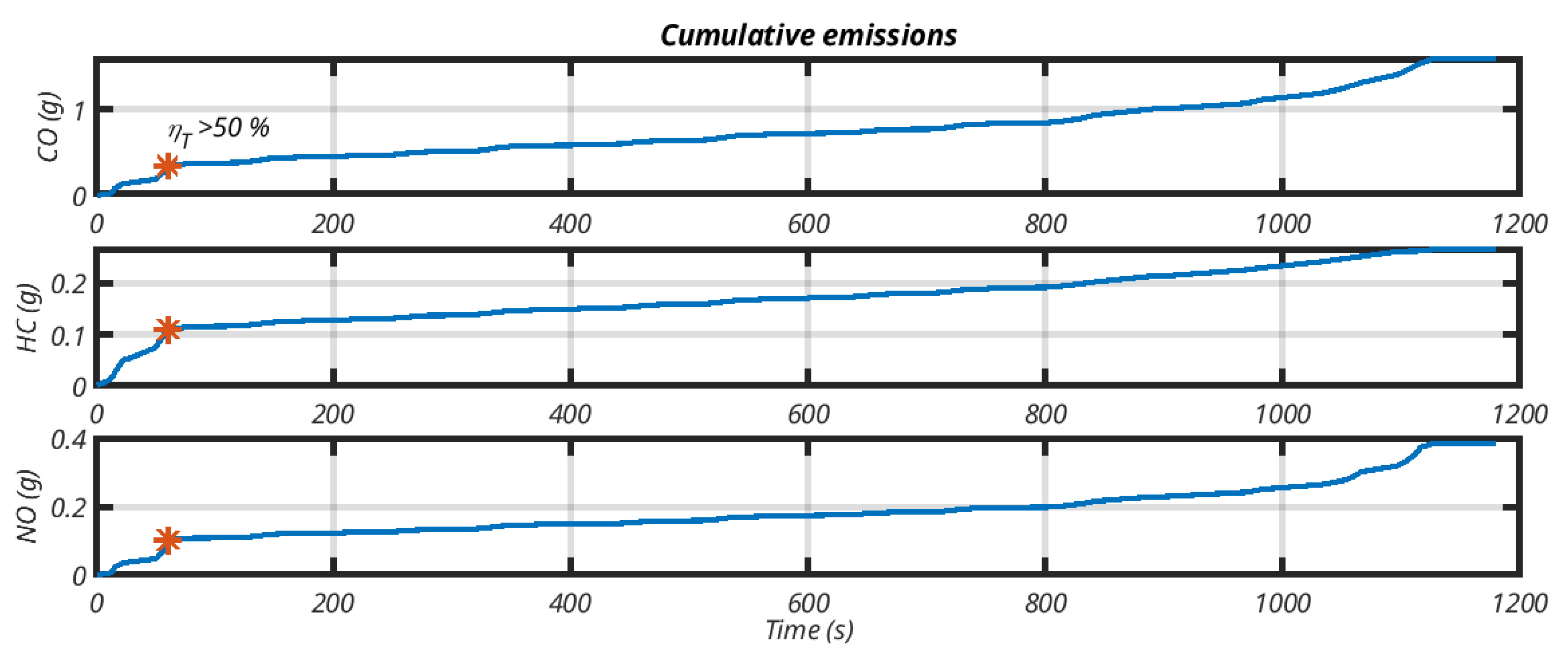
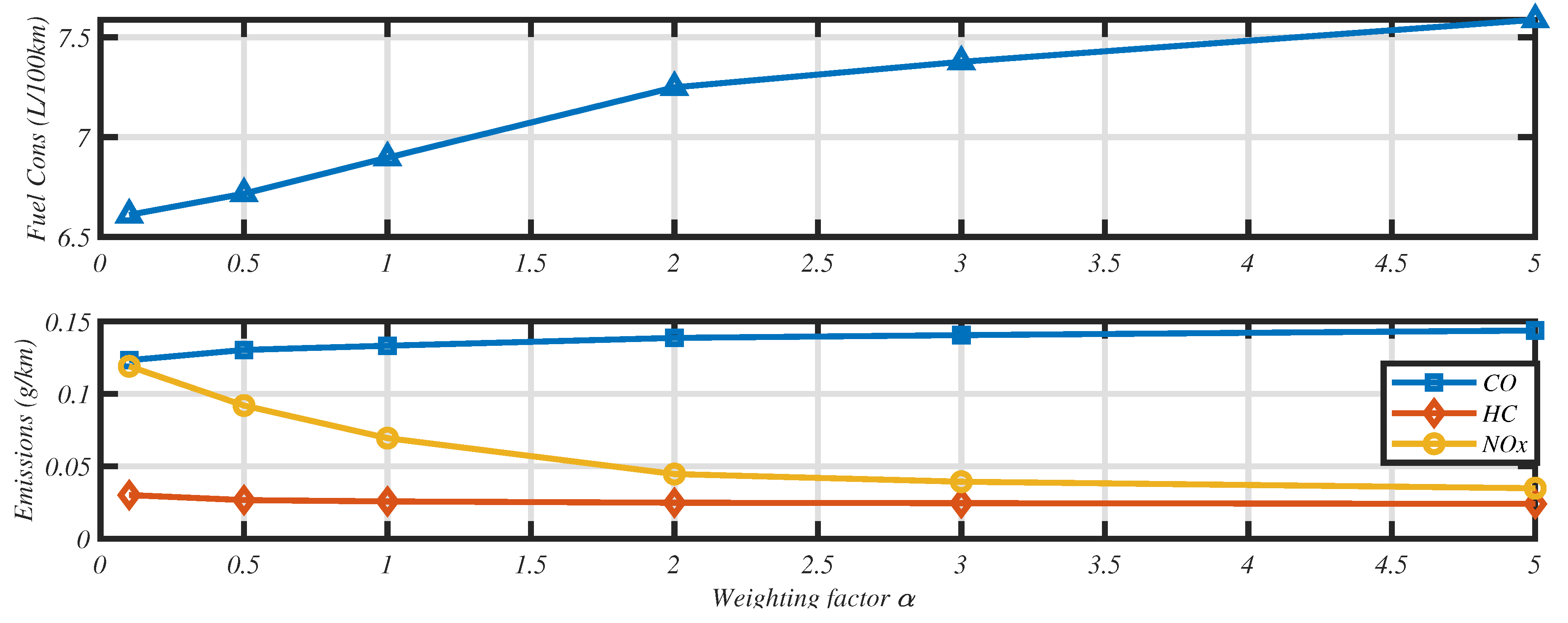
3.2. Trade-off between Fuel Consumption and Pollutant Emissions

In the previous section, we presented a pollution centered scenario where the weighting parameter $\alpha$ gives priority to pollutant emissions. In this section, we made several runs with different values of $\alpha$. This balances the fuel economy compared to pollutant emissions. Results are presented in Figure 27.

First, it can be noticed that a low weighting parameter ($\alpha =0.1$) of the objective function makes it possible to reduce pollutant emissions to a large extent without altering fuel consumption. In this case, the heating strategy of the catalyst is already implemented. With a hot catalyst, combustion is stoichiometric and a slight delay is observed compared to optimal spark advance (2° in this particular case).

When the value of $\alpha$ increases, NO emission can be further reduced by lowering exhaust gas temperature. As we can see in Figure 27, a good trade-off can be obtained by choosing a value of $\alpha$ between 1 and 2.

3.3. Worldwide Harmonized Light-Duty Vehicles Test Cycle

Figure 28 shows the vehicle speed and gearbox ratio during the WLTC that was used to validate the results on a more realistic and dynamic driving cycle.

Table 5. Performance of the pollution centered scenarios compared to the reference strategy (WLTC).

	Ref. Strategy ${\mathit{SA}}_{\mathit{opti}}$ $\mathit{\varphi }=1.0$	$\mathit{\alpha }=5$ $\mathit{SA}\mathit{var}$ $\mathit{\varphi }\mathit{var}$	Relative Variation
Consumption (L/100 km)	6.86	8.02	+17%
CO (g/km)	0.2554	0.128	−50%
HC (g/km)	0.029	0.013	−55%
NO (g/km)	0.179	0.040	−77%

and Figure 29 show a big improvement obtained with an appropriate strategy (gains ranging from 50 to almost 80% depending on the pollutant) while maintaining a good performance in fuel economy (17% increase in fuel consumption). Of course, here again, several trade-off between fuel consumption and emissions can be adopted.

First we notice in Figure 30 that both strategies present short light-off time: 75 s for the reference simulation, and only 19 s for the pollution centered scenario. These short times are the consequence of the more agressive dynamics of the drive cycle compared to NEDC. The strategy for the pollution centered scenario remains the same: significant deterioration of the spark advance (20 to 30° BTDC compared to optimal SA), and lean combustion ($\mathsf{\Phi }=0.9$). Throttle is full open. This induces an important exhaust flow at a high temperature.

When the catalyst is initiated, here again the strategies are similar to what happened during NEDC cycle: stoichiometric combustion, and slight delay of spark ignition in order to lower CO and NO concentrations.

4. Discussion

4.1. Originality of the Work

There is a great number of publications about catalyst behavior to satisfy more and more stringent emissions targets. Some authors focus on the three way catalyst model ([6,34,35,36]). Other authors work on minimizing one species during the cold start period ([37,38]). However, there is little literature that proposes trade-off between fuel consumption and pollutant emission during a whole drive cycle, without any empirical assumption of the duration of the cold start period nor arbitrary values for spark advance or lean/rich combustion.

Engine calibration is a critical step in the vehicle development process. Castagné et al. [4] make a comprehensive survey of different methods used to tune all calibration parameters. Every method is quite intensive and not completely satisfying. Most of the existing experimentally derived maps have not been optimized to be used for real-world applications. The model-based development appears to be a good process since it allows reducing the number of experiments with an intensive use of simulations. Developing engine and vehicle models that can be mathematically assisted with optimization methods can bring a solution to calibrate parameters. Moreover, rule-based maps can only represent the features of a specific engine, and hence, by a slight change in the ICE’s configuration, tedious design-of-experiment efforts should be repeated to revise the previous cold-start engine input maps. In this paper, we present a methodology that can be applied to every vehicle configuration.

In this sense, the tool presented in this paper can participate to the calibration task in two ways:

• defining the maps to be used by real time control strategies for both hot and cold catalyst
• serving as reference values for comparison with online methods

4.2. Discussion of the Method

An optimal control method allows calculating the best strategy, regarding the weighting parameter, with a steady-state formulation of the problem. This is an important fact since the optimization is made possible at the cost of simplifications such as neglecting certain state variables and their dynamics: we can cite the temperature rise of the cylinder head, which can induce high emissions of HC during a cold start period. We also neglect the wall wetting phenomena, typical in port fuel injection engines [39,40]. Certain portion of the fuel droplet would condense on the wall of the intake manifold, forming the fuel puddle, which has a significant impact on the mixture. Detrimental air to fuel ratio excursion could occur, giving rise to catalyst efficiency problems, particularly during transients.

Another important simplification is that all measurements have been made under steady-state operating conditions to feed the control model. However, any drive cycle includes transients during which steady-state engine behavior is not reached, leading to spikes in Lambda value. One can argue that part of these deviations can be partially mitigated by ${\mathrm{O}}_2$ storage in the catalyst [41].

4.3. Challenges and Limitations

The driving cycle has to be known in advance to establish the optimal energy management strategy with dynamic programming, which cannot be implemented in real vehicle. Other work focuses on the prediction of real-life driving cycle in order to adapt dynamic programming solutions to real-time control strategies [42]. Other approaches such as minimum Pontryaguin principle could be investigated and adapted in real time. However, one purpose of this algorithm is to ascertain the potential of reduction of pollutant emissions for conventional vehicles. It provides a reference of comparison to evaluate other sub optimal real-time strategies.

The generic functions developed in this paper have been derived from a specific data set from a particular engine. Nevertheless, for similar engine architectures, one can expect trends to be the same, although quantitatively there may be variations. The general optimization methodology and results presented here should therefore apply for SI engines with equivalent features. The units considered for pollutant models are concentrations, so an increase in the mass flow will naturally result in pollutants increase. Engine models introduce a displacement volume parameter, which can be used for scaling purposes. Next project will include the latest technologies for direct injection spark ignition engines (DISI) and corresponding control parameters in the optimization process (turbo charging, variable valve lifting, …). The models will be evolving with these new technologies.

A new objective will consist of adapting the algorithm to hybrid vehicles. Indeed, one can wonder if the additional degree of freedom brought by hybridization would change the engine management. From this perspective, a new state variable that represents the battery state of charge has to be introduced in the algorithm. We get three dimensions for the states (time, state of charge and catalyst temperature) and three dimensions for the control variables (intake pressure, spark advance and equivalence ratio). This is very challenging regarding to the use of computer’s memory and calculation time.

5. Conclusions

The original hypothesis of this work is that optimal control theory can provide information on how to drive the actuators of an internal combustion engine both during cold start and warmed catalyst. Indeed, the simulation results show that some trade-off can be found between fuel consumption and pollutant emissions. This is achieved in two ways: retarding the spark advance combined with a lean mixture to enhance catalyst ligth-off; keeping a slightly late ignition with a stoichiometric combustion as soon as catalyst is hot.

These findings are determined using two-dimensional dynamic programming with a weighted objective function. The entire model comprises eight sub-models and 35 tuning parameters. Each sub-model is based on semi-empirical assumptions. We take into account the thermal dynamics of the catalyst monolith, simple models for consumption, emissions and exhaust temperature. This decreases the computational burden while retaining the associated physical trends.

References

- European Environment Agency. Emissions of Air Pollutants from Transport; Technical Report; European Environment Agency: København, Denmark, 2019.
- Crippa, M.; Oreggioni, G.; Guizzardi, D.; Muntean, M.; Schaaf, E.; Lo Vullo, E.; Solazzo, E.; Monforti-Ferrario, F.; Olivier, J.; Vignati, E. Fossil CO2 and GHG Emissions of All World Countries: 2019 Report; Publications Office of the European Union: Luxembourg, 2019. [Google Scholar] [CrossRef]
- EU Commission Regulation. Framework Directive 2007/46/EC; Technical Report; European Union: Maastricht, The Netherlands, 2007.
- Castagné, M.; Bentolila, Y.; Chaudoye, F.; Hallé, A.; Nicolas, F.; Sinoquet, D. Comparison of Engine Calibration Methods Based on Design of Experiments (DoE). Oil Gas Sci. Technol. 2008, 63, 563–582. [Google Scholar] [CrossRef]
- Heywood, J.B. Internal Combustion Engine Fundamentals; McGraw-Hill Education: New York, NY, USA, 1988. [Google Scholar]
- Pandey, V.; Jeanneret, B.; Gillet, S.; Keromnes, A.; Le Moyne, L. A simplified thermal model for the three way catalytic converter. In Proceedings of the TAP 2016—21st International Transport and Air Pollution Conference, Lyon, France, 24–26 May 2016. [Google Scholar]
- Scordia, J.; Trigui, R.; Desbois-Renaudin, M.; Jeanneret, B.; Badin, F. Global Approach for Hybrid Vehicle Optimal Control. J. Asian Electr. Veh. 2009, 7, 1221–1230. [Google Scholar] [CrossRef]
- Vinot, E.; Scordia, J.; Trigui, R.; Jeanneret, B.; Badin, F. Model simulation, validation and case study of the 2004 THS of Toyota Prius. Int. J. Veh. Syst. Model. Test. 2008, 3, 139–167. [Google Scholar] [CrossRef]
- Lavoie, G.A.; Heywood, J.B.; Keck, J.C. Experimental and Theoretical Study of Nitric Oxide Formation in Internal Combustion Engines. Combust. Sci. Technol. 1970, 1, 313–326. [Google Scholar] [CrossRef]
- Kwon, H.; Choi, H.; Kim, J.; Min, K. Combustion and emission modelling of a direct-injection spark-ignition engine by combining flamelet models for premixed and diffusion flames. Combust. Theory Model. 2012, 16, 1089–1108. [Google Scholar] [CrossRef]
- Karvountzis-Kontakiotis, A.; Ntziachristos, L. Improvement of NO and CO predictions for a homogeneous combustion SI engine using a novel emissions model. Appl. Energy 2016, 162, 172–182. [Google Scholar] [CrossRef]
- Guzzella, L.; Onder, C.H. Introduction to Modeling and Control of Internal Combustion Engine Systems; Springer: Berlin/Heidelberg, Germany, 2010. [Google Scholar] [CrossRef]
- Abida, J.; Claude, D. Spark ignition engines and pollution emission: New approaches in modelling and control. Int. J. Veh. Des. 1994, 15, 494–508. [Google Scholar] [CrossRef]
- Sayin, C.; Ertunc, H.M.; Hosoz, M.; Kilicaslan, I.; Canakci, M. Performance and exhaust emissions of a gasoline engine using artificial neural network. Appl. Therm. Eng. 2007, 27, 46–54. [Google Scholar] [CrossRef]
- Nikzadfar, K.; Shamekhi, A.H. An extended mean value model (EMVM) for control-oriented modeling of diesel engines transient performance and emissions. Fuel 2015, 154, 275–292. [Google Scholar] [CrossRef]
- Andrianov, D.I.; Brear, M.J.; Manzie, C. A Physics-Based Integrated Model of a Spark Ignition Engine and a Three-Way Catalyst. Combust. Sci. Technol. 2012, 184, 1269–1301. [Google Scholar] [CrossRef]
- Shayler, P.J.; Chick, J.; Darnton, N.J.; Eade, D. Generic functions for fuel consumption and engine-out emissions of HC, CO and NOx of spark-ignition engines. Proc. Inst. Mech. Eng. Part D J. Automob. Eng. 1999, 213, 365–378. [Google Scholar] [CrossRef]
- Horrein, L.; Bouscayrol, A.; Delarue, P.; Verhille, J.; Mayet, C. Forward and Backward simulations of a power propulsion system. IFAC Proc. 2012, 45, 441–446. [Google Scholar] [CrossRef]
- Asus, Z.; Chrenko, D.; Aglzim, E.; Kéromnès, A.; Le Moyne, L. Simple method of estimating consumption of internal combustion engine for hybrid application. In Proceedings of the 2012 IEEE Transportation Electrification Conference and Expo (ITEC), Dearborn, MI, USA, 18–20 June 2012; pp. 1–6. [Google Scholar] [CrossRef]
- Guille des Buttes, A.; Jeanneret, B.; Kéromnès, A.; Le Moyne, L.; Pélissier, S. Energy management strategy to reduce pollutant emissions during the catalyst light-off of parallel hybrid vehicles. Appl. Energy 2020, 266, 114866. [Google Scholar] [CrossRef]
- Bowman, C.T. Kinetics of pollutant formation and destruction in combustion. Prog. Energy Combust. Sci. 1975, 1, 33–45. [Google Scholar] [CrossRef]
- Lakshminarayanan, P.A.; Aghav, Y.V. Hydrocarbon Emissions from Spark Ignition Engines. In Modelling Diesel Combustion; Springer Netherlands: Dordrecht, The Netherlands, 2010; pp. 147–166. [Google Scholar] [CrossRef]
- Zhao, L.; Yu, X.; Qian, D.C. The effects of EGR and ignition timing on emissions of GDI engine. Sci. China Technol. Sci. 2013, 56, 3144–3150. [Google Scholar] [CrossRef]
- Kaiser, E.; Siegl, W.; Brehob, D.; Haghgooie, M. Engine-Out Emissions from a Direct-Injection Spark-Ignition (DISI) Engine. SAE Trans. 1999, 108, 1155–1165. [Google Scholar]
- Raine, R.; Stone, C.; Gould, J. Modeling of nitric oxide formation in spark ignition engines with a multizone burned gas. Combust. Flame 1995, 102, 241–255. [Google Scholar] [CrossRef]
- Fenimore, C. Formation of nitric oxide in premixed hydrocarbon flames. Symp. (Int.) Combust. 1971, 13, 373–380. [Google Scholar] [CrossRef]
- Raimbault, V. Benefit of Air Intake Optimization for New Turbocharged Gasoline Engine. Ph.D. Thesis, Ecole Centrale de Nantes (ECN), Nantes, France, 2019. [Google Scholar]
- Yang, C.S.; Park, Y.J.; Cho, Y.; Kim, D.S. Variation of Exhaust Gas Temperature with the Change of Spark Timing and Exhaust Valve Timing During Cold Start Operation of an SI Engine. Trans. Korean Soc. Mech. Eng. B 2005, 29, 384–389. [Google Scholar] [CrossRef]
- Bordjane, M. Modélisation et Caractérisation Dynamique des Circuits d’admission et d’échappement des Moteurs à Combustion Interne. Ph.D. Thesis, Université des Sciences et de la Technologie Mohamed Boudiaf d’Oran, Oran, Maroc, 2013. [Google Scholar]
- Malkhede, D.N.; Khalane, H. Maximizing Volumetric Efficiency of IC Engine through Intake Manifold Tuning. In SAE 2015 World Congress and Exhibition; SAE International: Detroit, MI, USA, 23 April 2015. [Google Scholar] [CrossRef]
- Borman, G.; Nishiwaki, K. Internal-combustion engine heat transfer. Prog. Energy Combust. Sci. 1987, 13, 1–46. [Google Scholar] [CrossRef]
- Liu, F.; Akram, M.Z.; Wu, H. Hydrogen effect on lean flammability limits and burning characteristics of an isooctane–air mixture. Fuel 2020, 266, 117144. [Google Scholar] [CrossRef]
- Lumsden, G. Characterizing Engine Emissions with Spark Efficiency Curves. In SAE Technical Paper; SAE International: Tampa, FL, USA, 2004. [Google Scholar] [CrossRef]
- Brandt, E.P.; Grizzle, J.W. Three-way catalyst diagnostics for advanced emissions control systems. In Proceedings of the 2001 American Control Conference. (Cat. No.01CH37148), Arlington, VA, USA, 25–27 June 2001; Volume 5, pp. 3305–3311. [Google Scholar] [CrossRef]
- Sanketi, P.R.; Hedrick, J.K.; Kaga, T. A simplified catalytic converter model for automotive coldstart control applications. In Proceedings of the ASME 2005 International Mechanical Engineering Congress and Exposition, Orlando, FL, USA, 5–11 November 2005. [Google Scholar] [CrossRef]
- Tomforde, M.; Drewelow, W.; Duenow, P.; Lampe, B.; Schultalbers, M. A Post-Catalyst Control Strategy Based on Oxygen Storage Dynamics. In Proceedings of the SAE 2013 World Congress & Exhibition, Detroit, MI, USA, 16–18 April 2013. [Google Scholar] [CrossRef]
- Shaw, B.T.; Fisher, G.D.; Hedrick, J.K. A simplified coldstart catalyst thermal model to reduce hydrocarbon emissions. IFAC 2002, 35, 307–312. [Google Scholar] [CrossRef]
- Mozaffari, A.; Azad, N.L.; Hedrick, J.K. A Nonlinear Model Predictive Controller With Multiagent Online Optimizer for Automotive Cold-Start Hydrocarbon Emission Reduction. IEEE Trans. Veh. Technol. 2016, 65, 4548–4563. [Google Scholar] [CrossRef]
- Yildiz, Y.; Annaswamy, A.M.; Yanakiev, D.; Kolmanovsky, I. Spark ignition engine fuel-to-air ratio control: An adaptative control approach. Control. Eng. Pract. 2010, 18, 1369–1378. [Google Scholar] [CrossRef]
- Ye, Z.; Mohamadian, H. Model predictive control on wall wetting effect using Markov Chain Monte Carlo. In Proceedings of the 2013 IEEE Latin-America Conference on Communications, Santiago, Chile, 24–26 November 2013; pp. 1–6. [Google Scholar] [CrossRef]
- Muske, R.; Peyton-Jones, C. Estimating the oxygen storage level of a three way automotive catalyst. In Proceedings of the American Control Conference, Boston, MA, USA, 30 June–2 July 2004; Volume 35, pp. 4060–4065. [Google Scholar] [CrossRef]
- Joud, L.; Da Silva, R.; Chrenko, D.; Kéromnès, A.; Le Moyne, L. Smart Energy Management for Series Hybrid Electric Vehicles Based on Driver Habits Recognition and Prediction. Energies 2020, 13, 2954. [Google Scholar] [CrossRef]