
Incorporating Similarity Measures to Optimize Graph Convolutional Neural Networks for Product Recommendation


Abstract
:1. Introduction
- We propose a GCNN model for product recommendation that is based on the similarity among different nodes.
- We use the item click probability of a user to find their similarity with other users.
- We perform neighborhood sampling based on the similarity scores calculated through the KL divergence probability distribution formulation.
- The GCNN model is simplified by using neighbor modeling as a preprocessing step. The same neighbor modeling and embeddings learned are propagated through all the layers rather than the recursive aggregation of the neighbor’s data.
- We conducted experiments on two different datasets and used other proposed models to verify our proposed GCNN model’s performance. The results show that the proposed model performs better than the existing GCNN models and some traditional recommendation systems.
2. Related Work
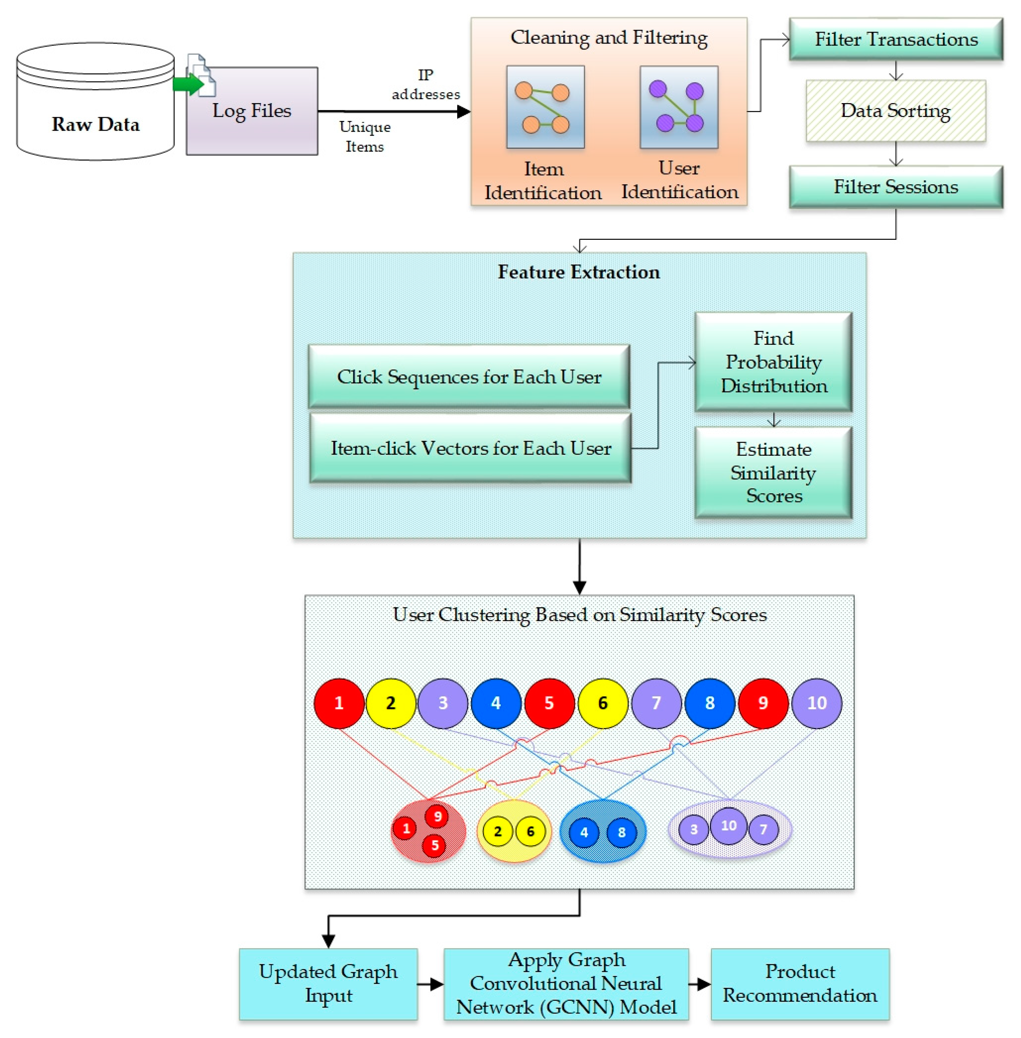
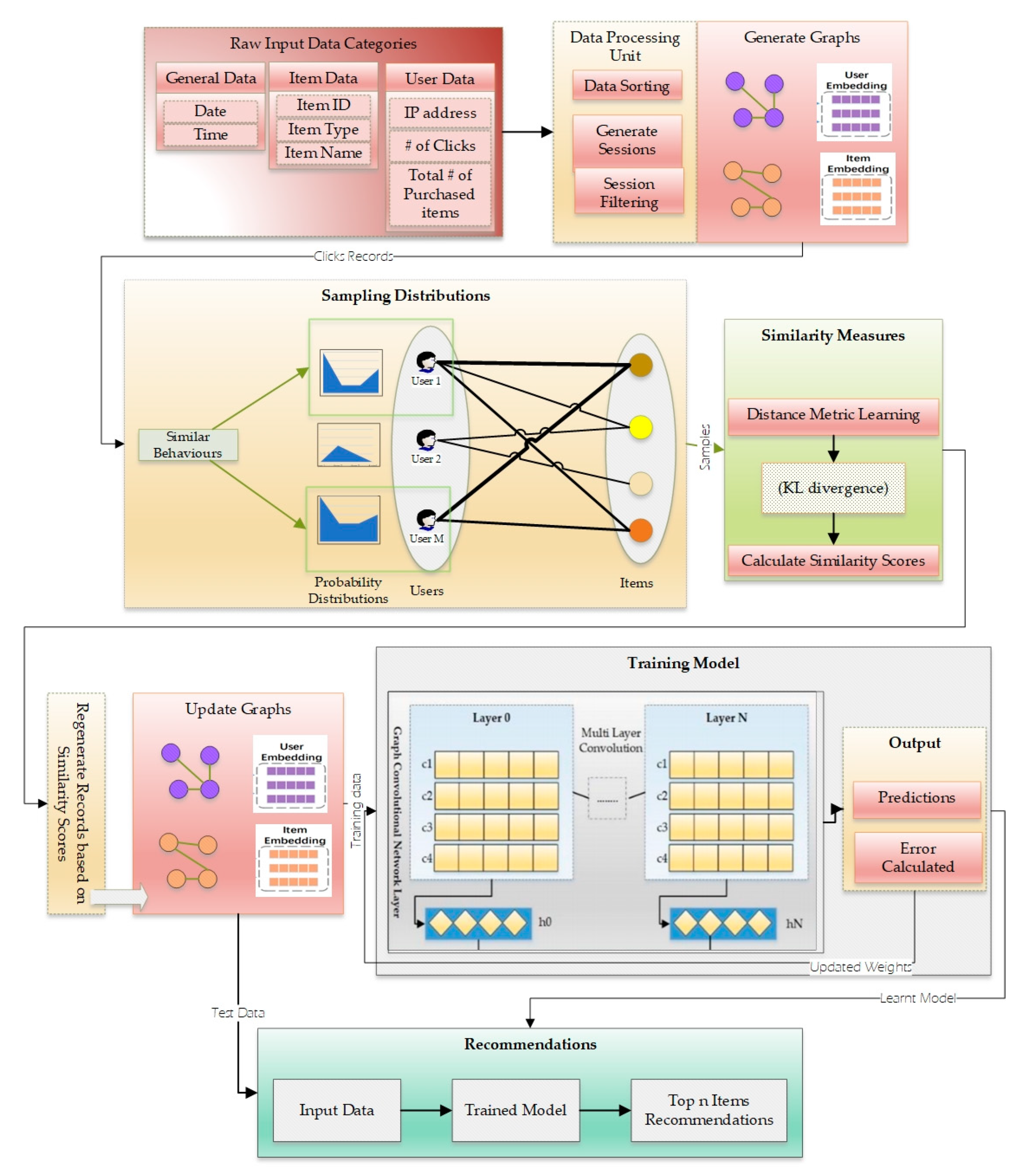
3. Proposed Model
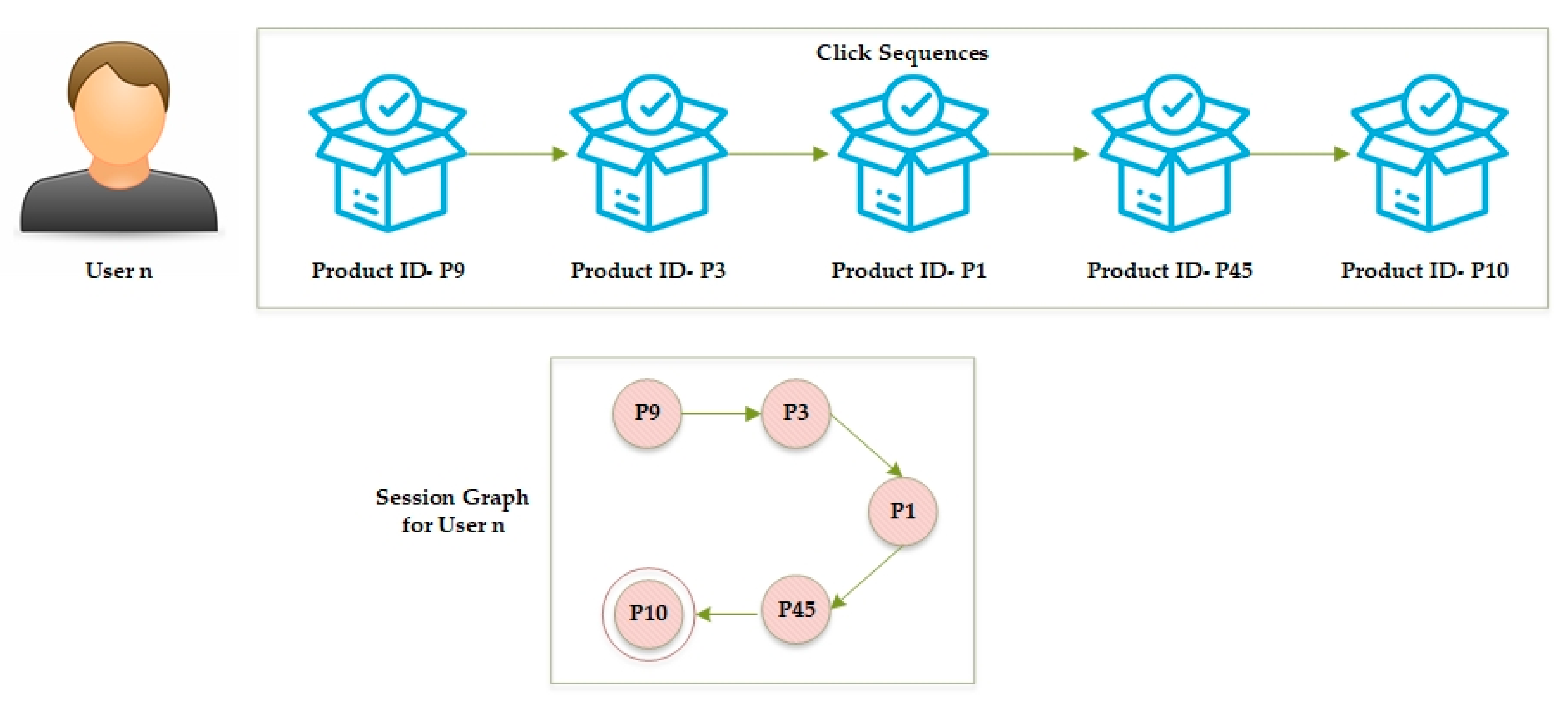
3.1. Problem Definition
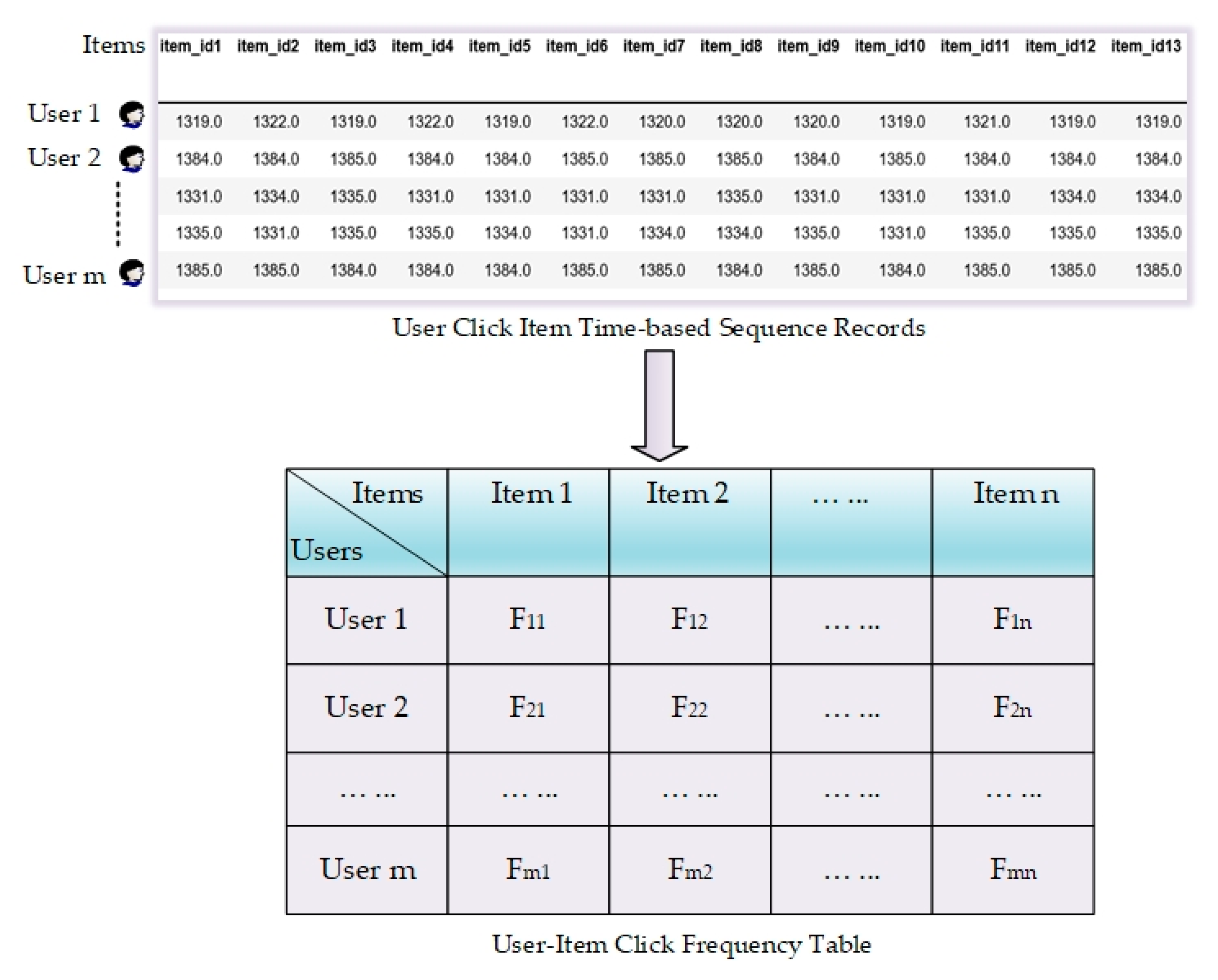
3.2. User–Item Click Frequency Table
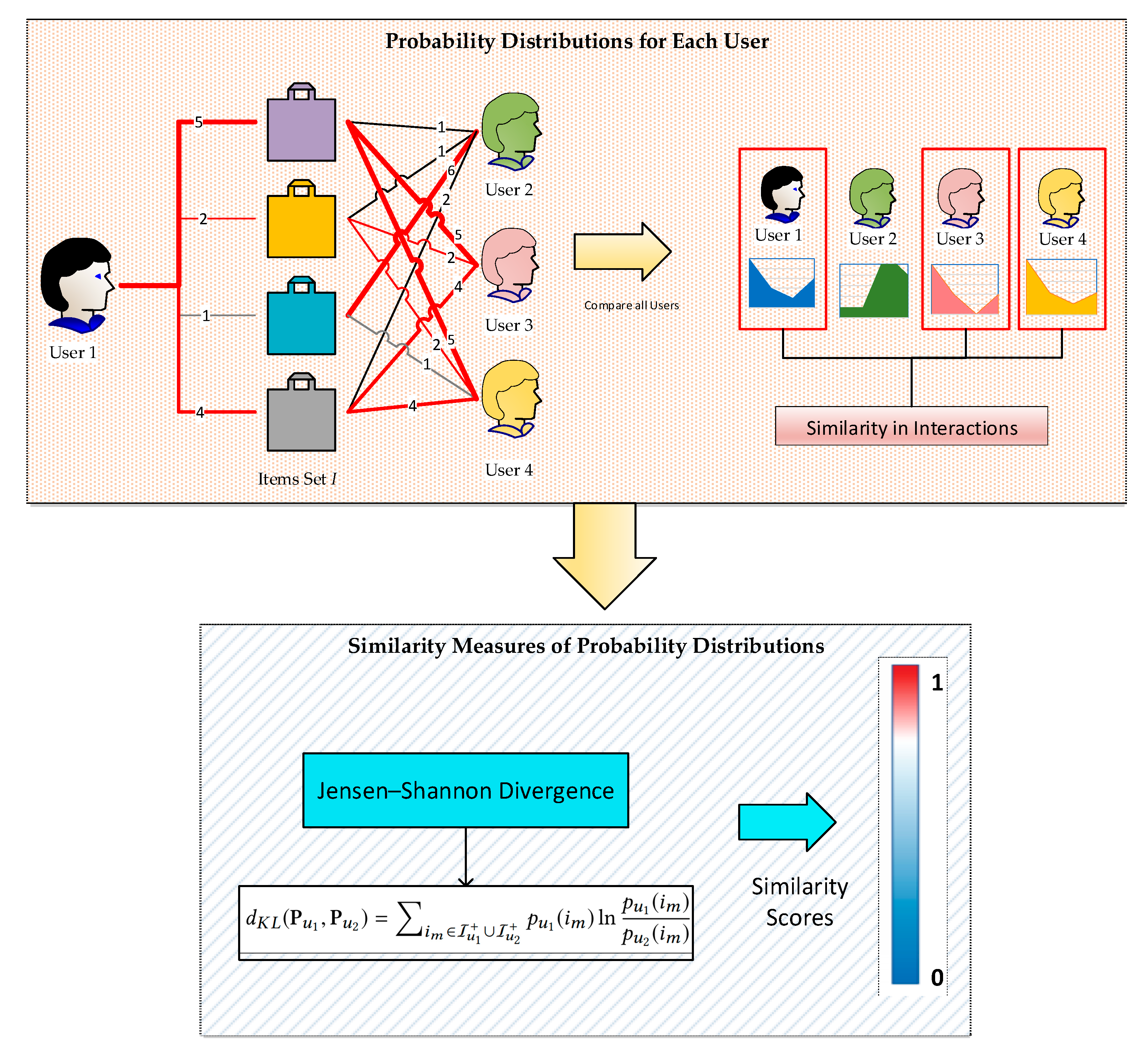
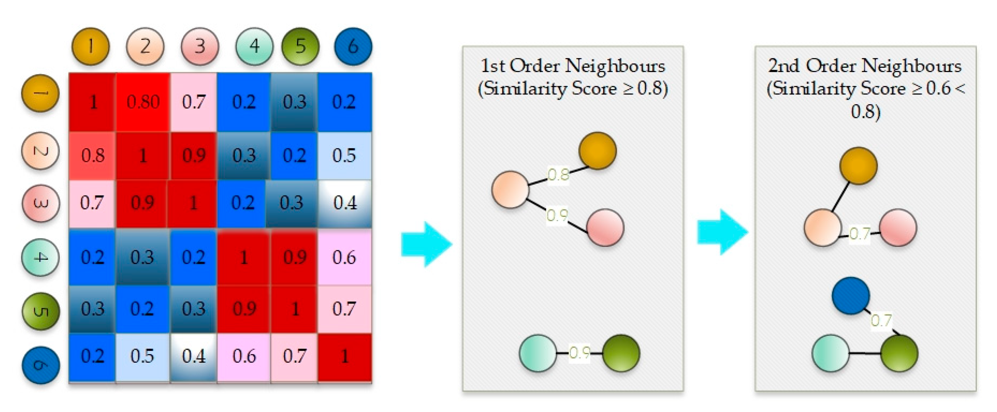
3.3. Measuring Similarity Based on Probability Distribution of User Interactions
3.4. GCNN-Based System Architecture
4. Data
4.1. Item Clicks of User
4.2. Customers’ Profile Data
4.3. Product Data
4.4. Experimental Data
5. Implementation and Experimental Setup
5.1. Experimental Setup
5.2. Evaluation Metrics
- Accuracy: the following formula was used to calculate the model’s accuracy, as shown in Equation (10).
- 2.
- Root Mean Square Error (RMSE): the RMSE was calculated using Equation (11).
- 3.
- Recall@20: This refers to the total number of correctly recommended items among the first 20 items, making this one of the essential evaluation metrics for building accurate recommendation systems.
- 4.
- F-Score: This analyzes the classification of a recommendation model and provides the model’s test accuracy computed from the precision and recall score.
- 5.
- MRR@20: This represents the mean reciprocal rank, and we computed the average reciprocal rank of the top 20 products. A higher value of MRR indicates that the model has higher accuracy for correctly recommending products.
- 6.
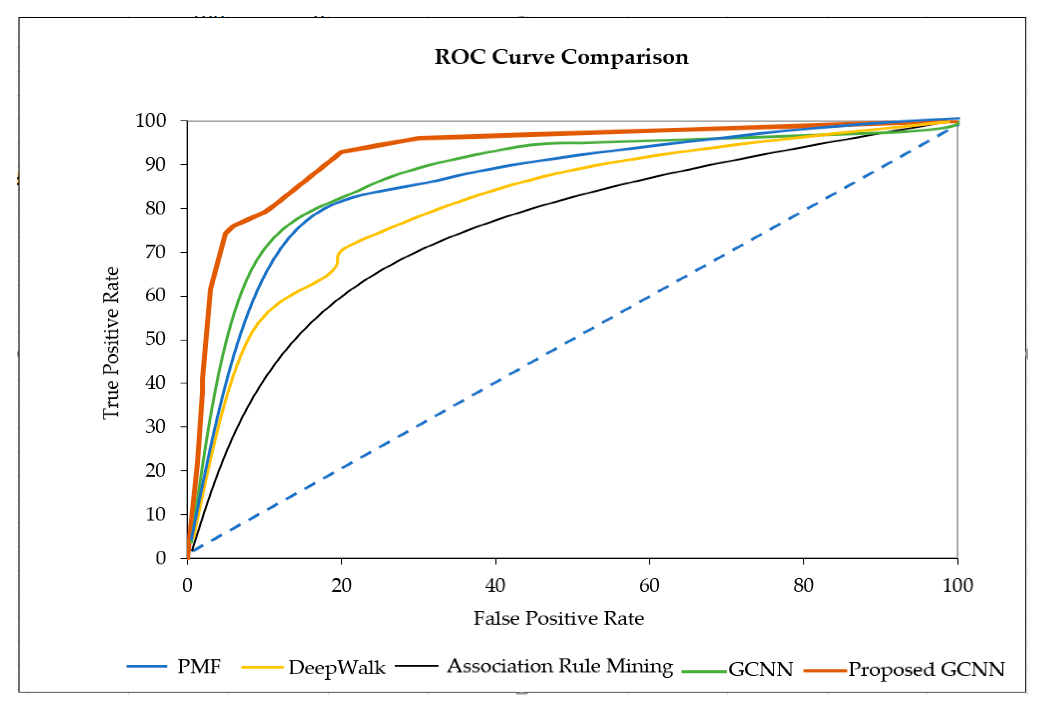
- ROC: The ROC curve (receiver operating characteristic curve) is a graph used to present the model’s classification performance. The two key parameters, known as the true-positive rate and false-positive rate, are plotted against each other. We used this performance metric to evaluate our model’s performance and compare it with a few traditional models.
6. Results
6.1. Comparison of Complexities and Convergence Rate
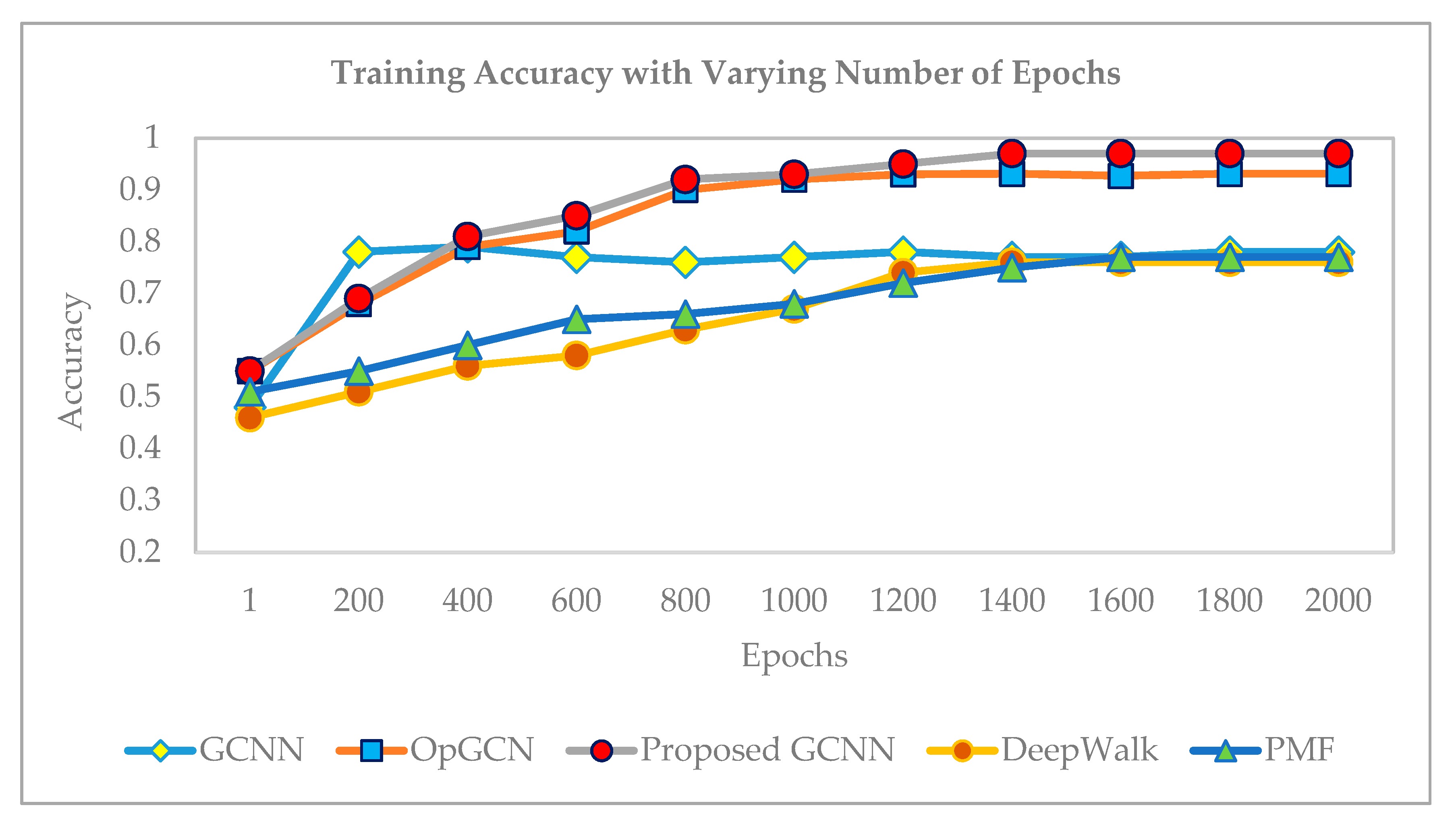
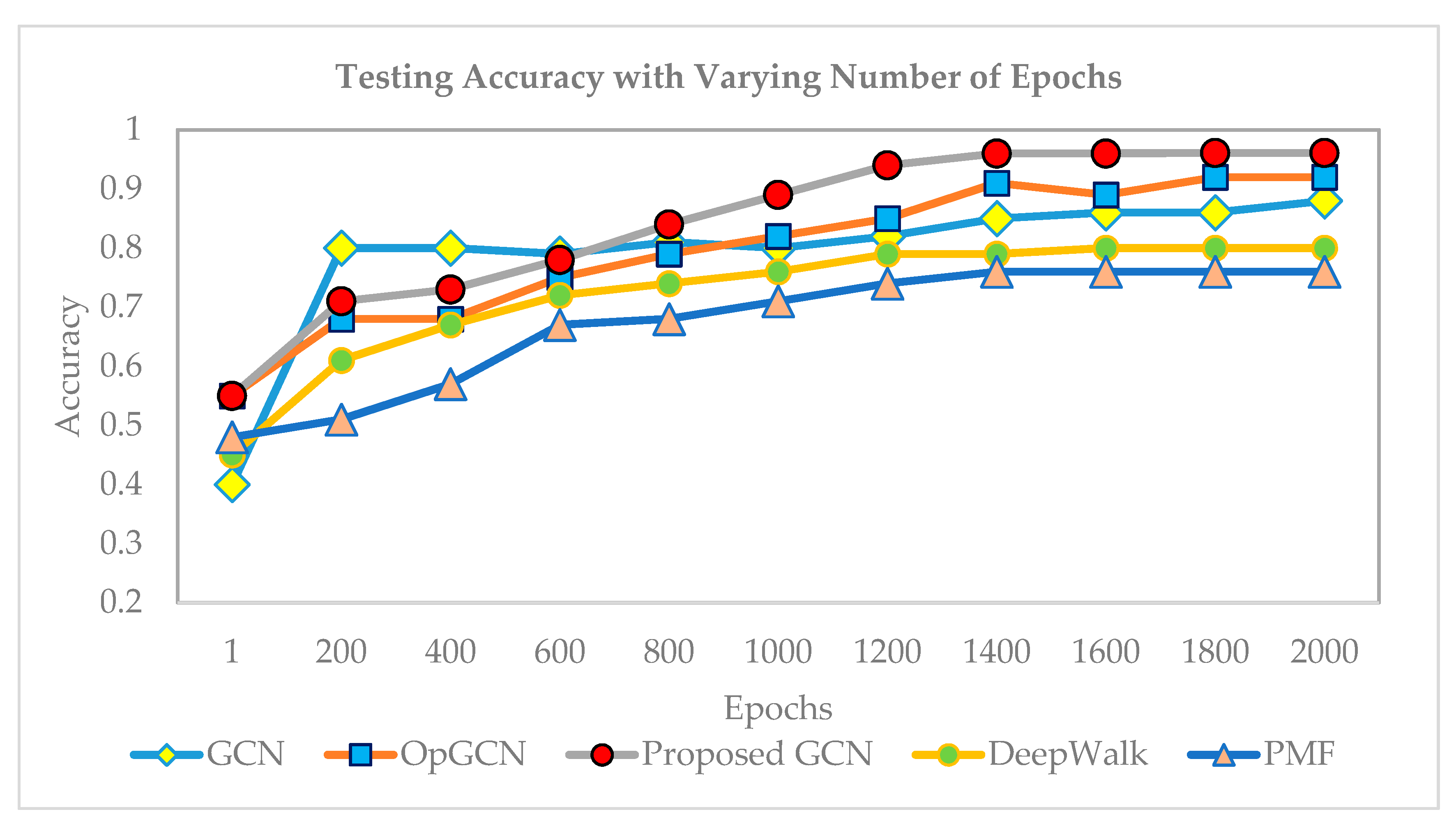
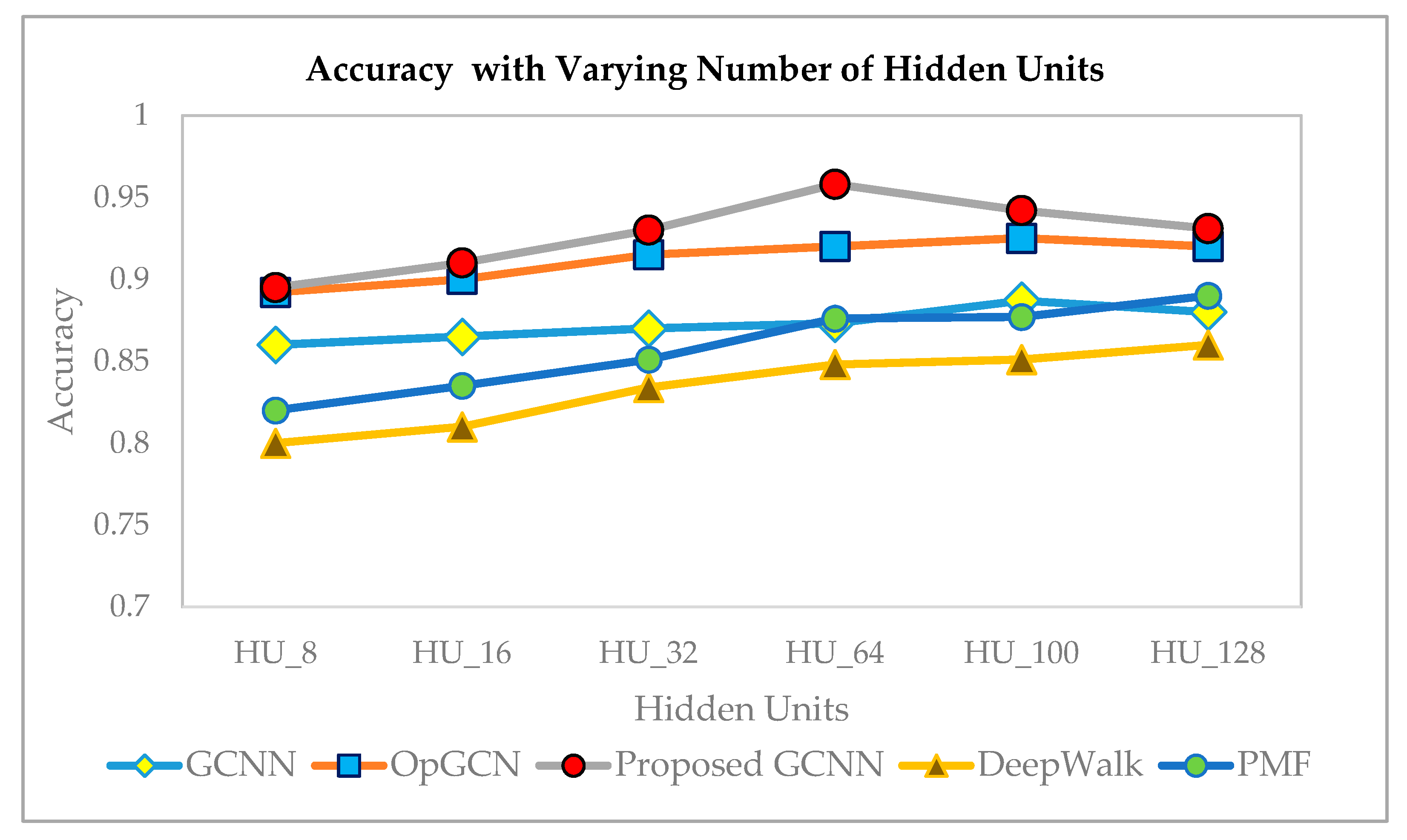
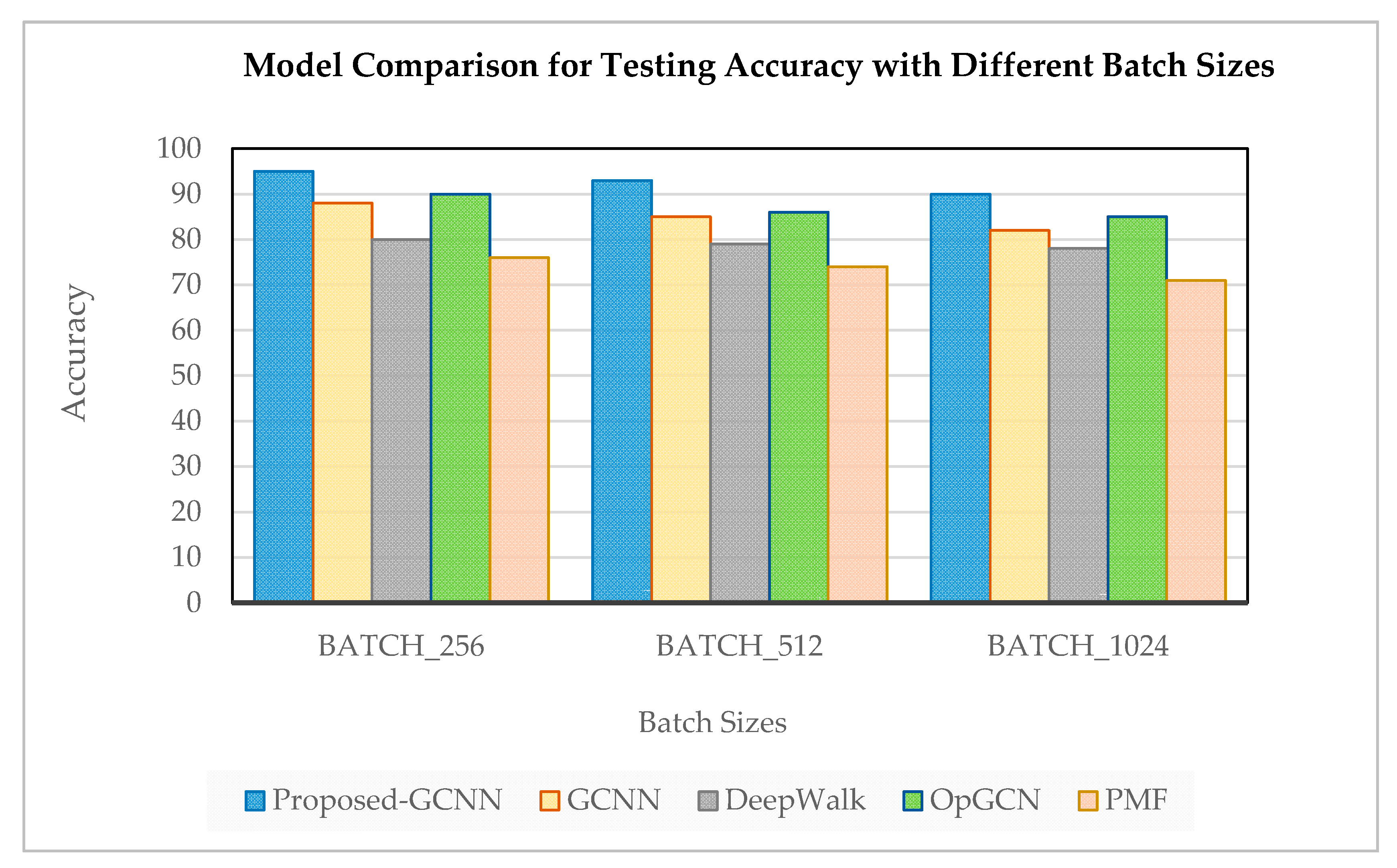
6.2. Training and Testing Accuracy
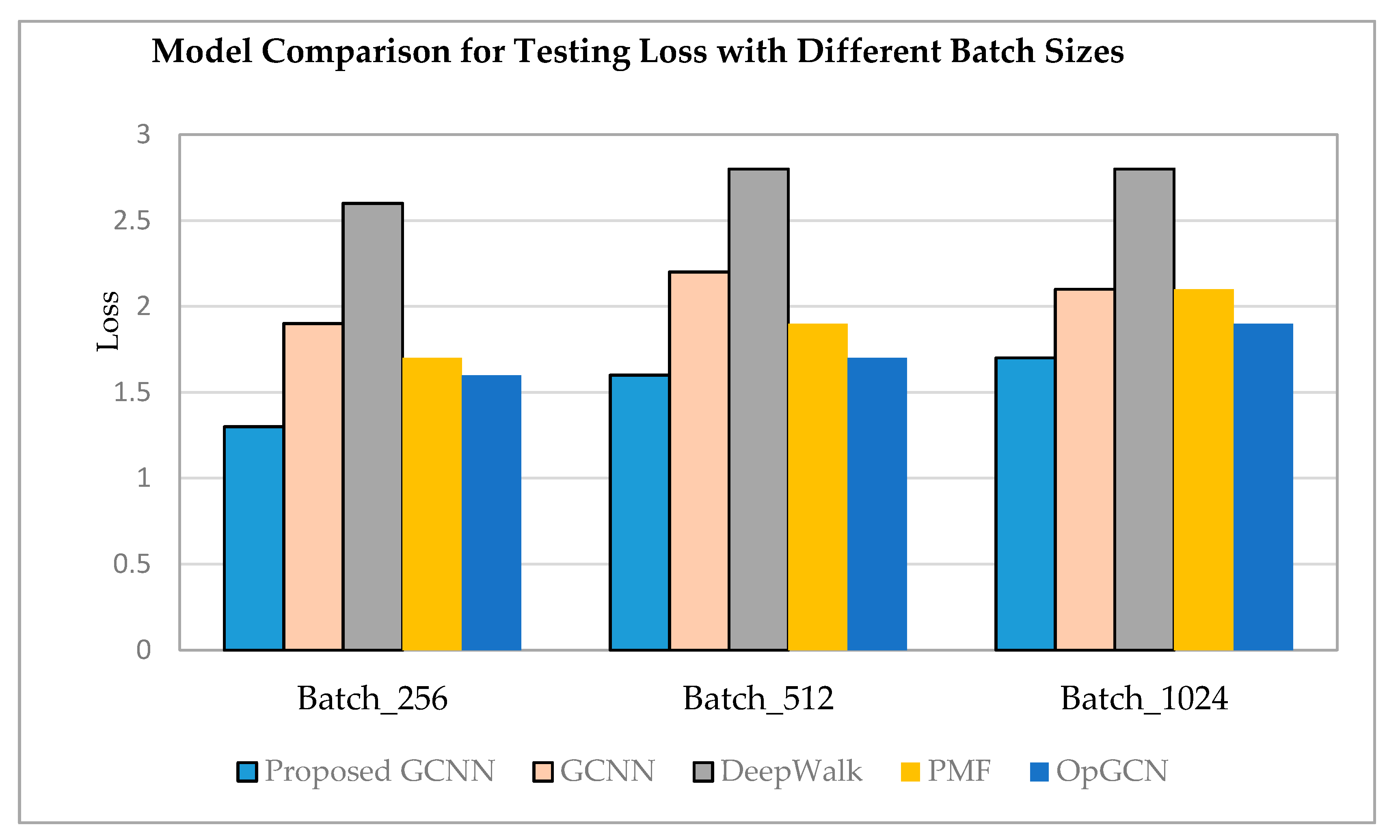
6.3. Loss for Training and Testing Model
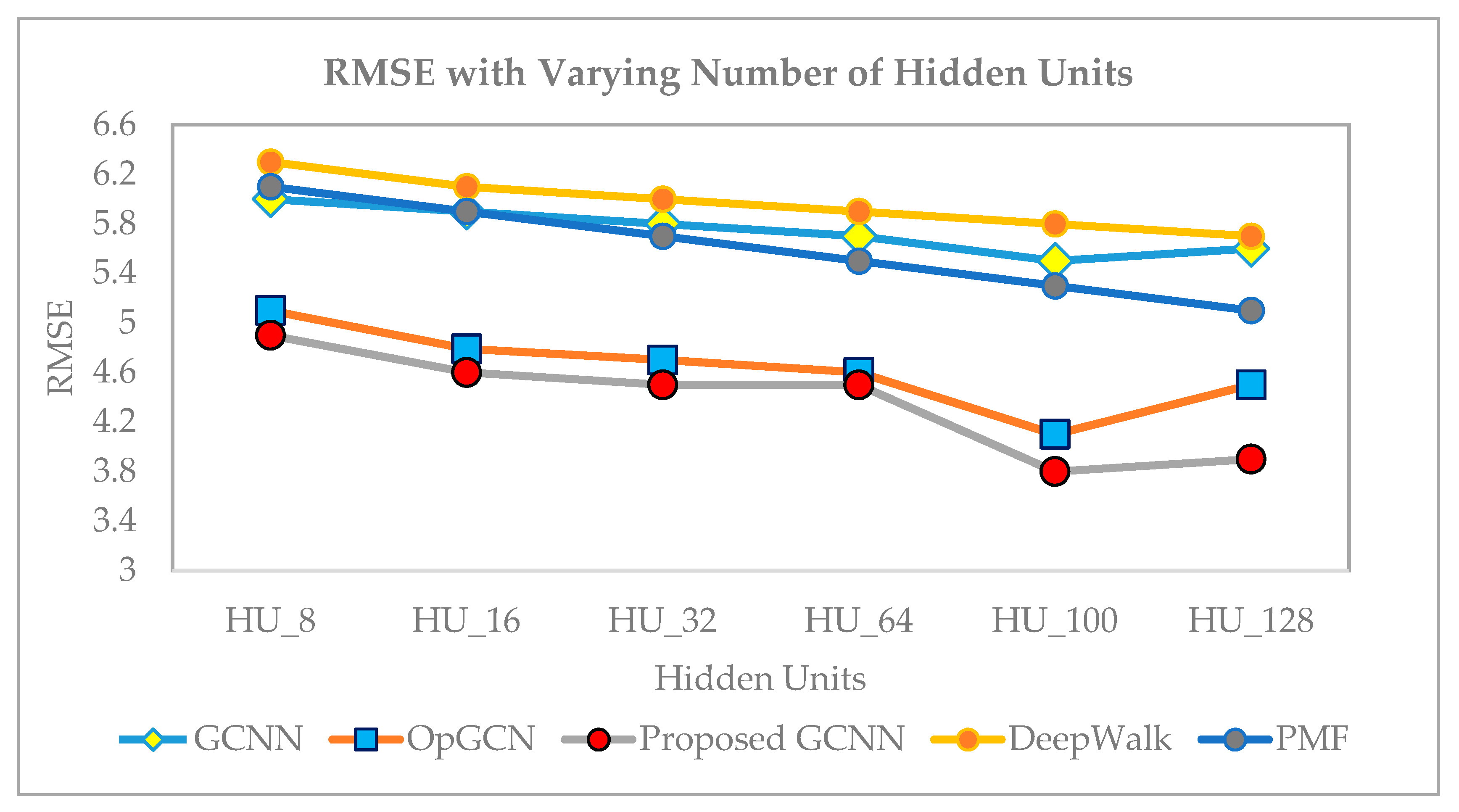
6.4. Error Score and ROC Comparisons
6.5. Performance Metric Comparisons of Different Models with Different Datasets
7. Conclusions
Author Contributions
Funding
Acknowledgments
Conflicts of Interest
References
- Alexander, J.E.; Tate, M.A. Web Wisdom: How to Evaluate and Create Web Page Quality; Erlbaum, L., Ed.; Associates Inc.: USA, 1999. [Google Scholar]
- Kräuter, S.G.; Kaluscha, E.A. Empirical research in on-line trust: A review and critical assessment. Int. J. Hum. Comput. Stud. 2003, 58, 783–812. [Google Scholar] [CrossRef]
- CROWDFUNDING MARKET-GROWTH, TRENDS, COVID-19 IMPACT, AND FORECASTS (2021–2026). Available online: https://www.mordorintelligence.com/industry-reports/crowdfunding-market (accessed on 2 December 2020).
- Crowdfunding. Available online: https://www.statista.com/outlook/335/100/crowdfunding/worldwide (accessed on 2 December 2020).
- Shih, Y.Y.; Liu, D.R. Product recommendation approaches: Collaborative filtering via customer lifetime value and customer demands. Expert Syst. Appl. 2008, 35, 350–360. [Google Scholar] [CrossRef]
- Liu, D.R.; Shih, Y.Y. Hybrid approaches to product recommendation based on customer lifetime value and purchase preferences. J. Syst. Softw. 2005, 77, 181–191. [Google Scholar] [CrossRef]
- Chen, H.; Yin, H.; Chen, T.; Nguyen, Q.V.H.; Peng, W.C.; Li, X. Exploiting Centrality Information with Graph Convolutions for Network Representation Learning. In Proceedings of the 2019 IEEE 35th International Conference on Data Engineering, Macau, China, 8–11 April 2019; pp. 590–601. [Google Scholar]
- He, X.; Deng, K.; Wang, X.; Li, Y.; Zhang, Y.D.; Wang, M. LightGCN: Simplifying and Powering Graph Convolution Network for Recommendation. arXiv 2020, arXiv:2002.02126. [Google Scholar]
- Wang, W.; Yin, H.; Huang, Z.; Wang, Q.; Du, X.; Nguyen, Q.V.H. Streaming Ranking Based Recommender Systems. In Proceedings of the 41st International ACM SIGIR Conference on Research & Development in Information Retrieval, Ann Arbor, MI, USA, 8–12 July 2018; pp. 525–534. [Google Scholar]
- Zhang, S.; Yao, L.; Sun, A.; Tay, Y. Deep learning based recommender system: A survey and new perspectives. ACM Comput. Surv. 2019, 5, 3285029. [Google Scholar] [CrossRef] [Green Version]
- Sedhain, S.; Menon, A.K.; Sanner, S.; Xie, L. Autorec: Autoencoders Meet Collaborative Filtering. In Proceedings of the 24th International Conference on World Wide Web 2015, Florence, Italy, 18–22 May 2015; pp. 111–112. [Google Scholar]
- Wu, Y.; DuBois, C.; Zheng, A.X.; Ester, M. Collaborative Denoising Auto-Encoders for Top-N Recommender Systems. In Proceedings of the Ninth ACM International Conference on Web Search and Data Mining CD-ROM, San Francisco, CA, USA, 22–25 February 2016; pp. 153–162. [Google Scholar]
- He, Q.; Pei, J.; Kifer, D.; Mitra, P.; Giles, L. Context-Aware Citation Recommendation. In Proceedings of the 19th International Conference on World Wide Web 2010, Raleigh, NC, USA, 26–30 April 2010; pp. 421–430. [Google Scholar]
- He, X.; Liao, L.; Zhang, H.; Nie, L.; Hu, X.; Chua, T.S. Neural collaborative filtering. World Wide Web Internet Web Inf. Syst. 2017, 173–182. [Google Scholar]
- Guo, H.; Tang, R.; Ye, Y.; Li, Z.; He, X. DeepFM: A factorization-machine based neural network for CTR prediction. IJCAI 2017, 1725–1731. [Google Scholar]
- Hsieh, C.K.; Yang, L.; Cui, Y.; Lin, T.Y.; Belongie, S.; Estrin, D. Collaborative Metric Learning. In Proceedings of the 26th International Conference on World Wide Web, Perth, Australia, 3–7 May 2017; pp. 193–201. [Google Scholar]
- Chen, J.; Xu, X.; Wu, Y.; Zheng, H. Gc-lstm: Graph convolution embedded lstm for dynamic link prediction. arXiv 2018, arXiv:1812.04206. [Google Scholar]
- Van den Berg, R.; Kipf, T.N.; Welling, M. Graph convolutional matrix completion. arXiv 2017, arXiv:1706.02263. [Google Scholar]
- Fan, W.; Ma, Y.; Li, Q.; He, Y.; Zhao, E.; Tang, J.; Yin, D. Graph Neural Networks for Social Recommendation. arXiv 2019, 1902, 07243. [Google Scholar]
- Ying, R.; He, R.; Chen, K.; Eksombatchai, P.; Hamilton, W.L.; Leskovec, J. Graph Convolutional Neural Networks for Web-Scale Recommender Systems. In Proceedings of the 24th ACM SIGKDD International Conference on Knowledge Discovery and Data Mining, London, UK, 19–23 August 2018; pp. 974–983. [Google Scholar]
- Chami, I.; Ying, Z.; Ré, C.; Leskovec, J. Hyperbolic Graph Convolutional Neural Networks. In Proceedings of the 2019 Conference on Neural Information Processing Systems, Vancouver, BC, Canada, 8–14 December 2019; pp. 4869–4880. [Google Scholar]
- Zhang, M.; Chen, Y. Link Prediction Based on Graph Neural Networks. In Proceedings of the 2018 Conference on Neural Information Processing Systems, Montreal, QC, Canada, 3–8 December 2018; pp. 5165–5175. [Google Scholar]
- Chen, J.; Ma, T.; Xiao, C. FastGCN: Fast Learning with Graph Convolutional Networks via Importance Sampling. In Proceedings of the 6th International Conference on Learning Representations, Vancouver, BC, Canada, 30 April–3 May 2018. [Google Scholar]
- Hamilton, W.; Ying, Z.; Leskovec, J. Inductive Representation Learning on Large Graphs. In Proceedings of the 2017 Conference on Neural Information Processing Systems, Long Beach, CA, USA, 4–9 December 2017; pp. 1024–1034. [Google Scholar]
- Veličković, P.; Cucurull, G.; Casanova, A.; Romero, A.; Lio, P.; Bengio, Y. Graph Attention Networks. In Proceedings of the 6th International Conference on Learning Representations, Vancouver, BC, Canada, 30 April–3 May 2018. [Google Scholar]
- Zhao, H.; Yao, Q.; Li, J.; Song, Y.; Lee, D.L. Metagraph Based Recommendation Fusion Over Heterogeneous Information Networks. In Proceedings of the 23rd ACM SIGKDD International Conference on Knowledge Discovery and Data Mining, Halifax, NS, Canada, 13–17 August 2017; pp. 635–644. [Google Scholar]
- Zhao, J.; Zhou, Z.; Guan, Z.; Zhao, W.; Ning, W.; Qiu, G.; He, X. IntentGC: A Scalable Graph Convolution Framework Fusing Heterogeneous Information for Recommendation. In Proceedings of the 25th ACM SIGKDD International Conference on Knowledge Discovery & Data Mining, Anchorage, AK, USA, 4–8 August 2019; pp. 2347–2357. [Google Scholar]
- Hu, B.; Shi, C.; Zhao, W.X.; Yu, P.S. Leveraging Meta-Path Based Context for Top-N Tecommendation with A Neural Co-Attention Model. In Proceedings of the 24th ACM SIGKDD International Conference on Knowledge Discovery & Data Mining, London, UK, 19–23 August 2018; pp. 1531–1540. [Google Scholar]
- Wu, Q.; Zhang, H.; Gao, X.; He, P.; Weng, P.; Gao, H.; Chen, G. Dual Graph Attention Networks for Deep Latent Representation of Multifaceted Social Effects in Recommender Systems. In Proceedings of the International World Wide Web Conferences, San Francisco, CA, USA, 13–17 May 2019; pp. 2091–2102. [Google Scholar]
- Shafqat, W.; Byun, C.Y. Enabling “Untact” Culture via Online Product Recommendations: An Optimized Graph-CNN based Approach. Appl. Sci. 2020, 10, 5445. [Google Scholar] [CrossRef]
- Wu, F.; Zhang, T.; de Souza, A.H., Jr.; Fifty, C.; Yu, T.; Weinberger, K.Q. Simplifying Graph Convolutional Networks. In Proceedings of the 2019 International Conference on Machine Learning, Long Beach, CA, USA, 10–15 June 2019. [Google Scholar]
- Budhiraja, A.; Hiranandani, G.; Yarrabelly, N.; Choure, A.; Koyejo, O.; Jain, P. Rich-Item Recommendations for Rich-Users via GCNN: Exploiting Dynamic and Static Side Information. arXiv 2020, arXiv:2001.10495. [Google Scholar]
- Jianing, S.; Zhang, Y.; Ma, C.; Coates, M.; Guo, H.; Tang, R.; He, X. Multi-Graph Convolution Collaborative Filtering. In Proceedings of the 2019 IEEE International Conference on Data Mining, Beijing, China, 8–11 November 2019; pp. 1306–1311. [Google Scholar]
- Zhiwei, L.; Wan, M.; Guo, S.; Achan, K.; Yu, P.S. BasConv: Aggregating Heterogeneous Interactions for Basket Recommendation with Graph Convolutional Neural Network. In Proceedings of the 2020 SIAM International Conference on Data Mining, Cincinnati, OH, USA, 7–9 May 2020; pp. 64–72. [Google Scholar]
- Tong, Z.; Cui, B.; Cui, Z.; Huang, H.; Yang, J.; Deng, H.; Zheng, B. Cross-Graph Convolution Learning for Large-Scale Text-Picture Shopping Guide in E-Commerce Search. In Proceedings of the 2020 IEEE 36th International Conference on Data Engineering (ICDE), Dallas, TX, USA, 20–24 April 2020; pp. 1657–1666. [Google Scholar]
- Lee, H.; Lee, J. Scalable deep learning-based recommendation systems. ICT Express 2019, 5, 84–88. [Google Scholar] [CrossRef]
- Aminu, D.; Salim, N.; Rabiu, I.; Osman, A. Recommendation system exploiting aspect-based opinion mining with deep learning method. Inf. Sci. 2020, 512, 1279–1292. [Google Scholar]
- Kipf, T.N.; Welling, M. Semi-Supervised Classification with Graph Convolutional Networks. In Proceedings of the 5th International Conference on Learning Representations, Toulon, France, 24–26 April 2017. [Google Scholar]
- Schlichtkrull, M.S.; Kipf, T.N.; Bloem, P.; van den Berg, R.; Titov, I.; Welling, M. Modeling Relational Data with Graph Convolutional Networks. In Proceedings of the Semantic Web—15th International Conference, Heraklion, Crete, Greece, 3–7 June 2018; pp. 593–607. [Google Scholar]
- Hamilton, W.L.; Ying, Z.; Leskovec, J. Inductive Representation Learning on Large Graphs. In Advances in Neural Information Processing Systems 30, Proceedings of the Annual Conference on Neural Information Processing Systems 2017, Long Beach, CA, USA, 4–9 December 2017; Neural Information Processing Systems Foundation Inc.: La Jolla, CA, USA, 2017; pp. 1025–1035. [Google Scholar]
- Huang, W.B.; Zhang, T.; Rong, Y.; Huang, J. Adaptive Sampling towards Fast Graph Representation Learning. In Advances in Neural Information Processing Systems 31, Proceedings of the Annual Conference on Neural Information Processing Systems 2018, NeurIPS 2018, Montréal, QC, Canada, 3–8 December 2018; Neural Information Processing Systems Foundation Inc.: La Jolla, CA, USA, 2018; pp. 4563–4572. [Google Scholar]
- Chiang, W.L.; Liu, X.; Si, S.; Li, Y.; Bengio, S.; Hsieh, C.J. Cluster-gcn: An Efficient Algorithm for Training Deep and Large Graph Convolutional Networks. In Proceedings of the 25th ACM SIGKDD International Conference on Knowledge Discovery & Data Mining, Anchorage, AK, USA, 4–8 August 2019; pp. 257–266. [Google Scholar]
- Chen, J.; Zhu, J.; Song, L. Stochastic Training of Graph Convolutional Networks with Variance Reduction. In Proceedings of the 35th International Conference on Machine Learning, Stockholm, Sweden, 10–15 July 2018; pp. 941–949. [Google Scholar]
- Fan, S.; Zhu, J.; Han, X.; Shi, C.; Hu, L.; Ma, B.; Li, Y. Metapath-Guided Heterogeneous Graph Neural Network for Intent Recommendation. In Proceedings of the 25th ACM SIGKDD International Conference on Knowledge Discovery & Data Mining, Anchorage, AK, USA, 4–8 August 2019; pp. 2478–2486. [Google Scholar]
- Nielsen, F. On the Jensen–Shannon symmetrization of distances relying on abstract means. Entropy 2019, 21, 485. [Google Scholar] [CrossRef] [PubMed] [Green Version]
- Feng, L.; Wang, H.; Jin, B.; Li, H.; Xue, M.; Wang, L. Learning a distance metric by balancing kl-divergence for imbalanced datasets. IEEE Trans. Syst. Man Cybern. Syst. 2018, 49, 2384–2395. [Google Scholar] [CrossRef]
- Kaggle, RecSys Challenge 2015. Available online: https://www.kaggle.com/chadgostopp/recsys-challenge-2015 (accessed on 10 November 2020).
- CodaLab, CIKM Cup 2016 Track 2: Personalized E-Commerce Search Challenge. Available online: https://competitions.codalab.org/competitions/11161 (accessed on 10 November 2020).
- Perozzi, B.; Rfou, R.A.; Skiena, S. DeepWalk: Online learning of social representations. arXiv 2014, arXiv:1403.6652. [Google Scholar]
- Wang, H.; Zhao, M.; Xie, X.; Li, W.; Guo, M. Knowledge Graph Convolutional Networks for Recommender Systems. In Proceedings of the World Wide Web Conference 2019, San Francisco, CA, USA, 13–17 May 2019; pp. 3307–3313. [Google Scholar]
- Mnih, A.; Salakhutdinov, R.R. Probabilistic Matrix Factorization. In Advances in Neural Information Processing Systems; MIT Press: Vancouver, BC, Canada, 2007; Volume 20, pp. 1257–1264. [Google Scholar]
- Sandvig, J.J.; Mobasher, B.; Burke, R. Robustness of Collaborative Recommendation Based on Association Rule Mining. In Proceedings of the 2007 ACM Conference on Recommender Systems, Minneapolis, MN, USA, 19–20 October 2007; pp. 105–112. [Google Scholar]
- Koren, Y. Factorization Meets the Neighborhood: A Multifaceted Collaborative Filtering Model. In Proceedings of the 14th ACM SIGKDD International Conference on Knowledge Discovery and Data Mining, Las Vegas, NV, USA, 24–27 August 2008; pp. 426–434. [Google Scholar]


| Notations | Definitions |
|---|---|
| U | Set of all users |
| I | Set of all products |
| () | Click probability of user m for item i |
| (I) | Click probability of user m for all items I |
| The similarity between two users u1 and u2 | |
| Set of user ui’s clicked items | |
| Union set of all the items in any of two users from U consisting of clicked items |
| Data | Definition |
|---|---|
| User IP address | |
| The date when user accessed the website | |
| The time when the user accessed the website | |
| URL of the specific page accessed by the user | |
| The ID of the product clicked by the user | |
| Name of the product clicked by the user | |
| Type of the product clicked by the user |
| Data | Statistics |
|---|---|
| Total number of instances | ~300 K |
| Period of data | One Year (2019–2020) |
| Number of unique customers | ~50 K |
| Total purchased products | 7701 |
| Total number of unique clicks | 244,533 |
| Total number of visited item description pages | 42 K |
| Model | Time Complexity | Memory Complexity | Convergence Rate |
|---|---|---|---|
| DeepWalk | O (Lneh.log(n)) | O (Lnh + Lh2) | 2200 Epochs |
| KGCN-Neighbour | O (Leh + Lnh2 + rLnh2) | O (Lnh + Lh2) | 2100 Epochs |
| GCNN | O (Leh + Lnh2) | O (Lnh + Lh2) | 1800 Epochs |
| OpGCN | O (Lrnh2) | O (Lbrh + Lh2) | 1650 Epochs |
| Proposed GCNN | O (Leh + Lnh2) | O (Lbh + Lh2) | 1400 Epochs |
| Data | Metrics | SVD | KGCN-Neighbor | DeepWalk | Association Rule Mining | GCNN | OpGCN | Proposed GCNN |
|---|---|---|---|---|---|---|---|---|
| YOOCHOOSE | Recall@20 | 17.19 | 28.31 | 45.16 | 31.19 | 50.64 | 69.48 | 70.18 |
| F-Score | 0.617 | 0.669 | 0.712 | 0.613 | 0.718 | 0.841 | 0.892 | |
| MRR@20 | 8.11 | 19.21 | 17.59 | 27.83 | 37.15 | 38.12 | 40.55 | |
| Testing Accuracy | 0.65 | 0.69 | 0.71 | 0.61 | 0.77 | 0.76 | 0.81 | |
| DIGINETICA | Recall@20 | 20.13 | 27.44 | 46.98 | 31.26 | 48.13 | 65.42 | 69.87 |
| F-Score | 0.691 | 0.627 | 0.698 | 0.713 | 0.785 | 0.794 | 0.847 | |
| MRR@20 | 9.19 | 20.18 | 17.11 | 25.56 | 34.13 | 37.40 | 39.98 | |
| Testing Accuracy | 0.68 | 0.72 | 0.77 | 0.74 | 0.82 | 0.86 | 0.93 | |
| Our Data | Recall@20 | 20.21 | 29.82 | 45.38 | 38.56 | 50.18 | 69.34 | 78.91 |
| F-Score | 0.647 | 0.624 | 0.791 | 0.792 | 0.869 | 0.856 | 0.914 | |
| MRR@20 | 8.02 | 19.34 | 20.45 | 28.01 | 39.11 | 37.14 | 39.17 | |
| Testing Accuracy | 0.61 | 0.72 | 0.75 | 0.75 | 0.81 | 0.88 | 0.97 |
Publisher’s Note: MDPI stays neutral with regard to jurisdictional claims in published maps and institutional affiliations. |
© 2021 by the authors. Licensee MDPI, Basel, Switzerland. This article is an open access article distributed under the terms and conditions of the Creative Commons Attribution (CC BY) license (http://creativecommons.org/licenses/by/4.0/).
Share and Cite
Shafqat, W.; Byun, Y.-C. Incorporating Similarity Measures to Optimize Graph Convolutional Neural Networks for Product Recommendation. Appl. Sci. 2021, 11, 1366. https://doi.org/10.3390/app11041366
Shafqat W, Byun Y-C. Incorporating Similarity Measures to Optimize Graph Convolutional Neural Networks for Product Recommendation. Applied Sciences. 2021; 11(4):1366. https://doi.org/10.3390/app11041366
Chicago/Turabian StyleShafqat, Wafa, and Yung-Cheol Byun. 2021. "Incorporating Similarity Measures to Optimize Graph Convolutional Neural Networks for Product Recommendation" Applied Sciences 11, no. 4: 1366. https://doi.org/10.3390/app11041366