Underwater Acoustic Target Recognition with a Residual Network and the Optimized Feature Extraction Method


Abstract
1. Introduction
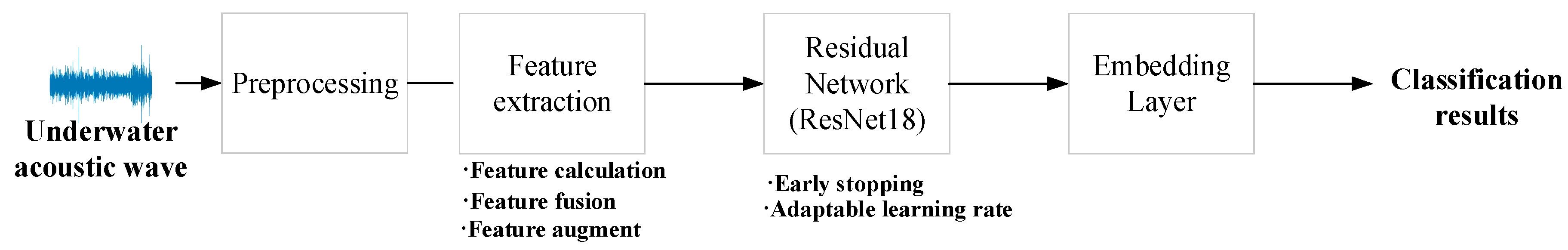
2. Description of the Classification Method
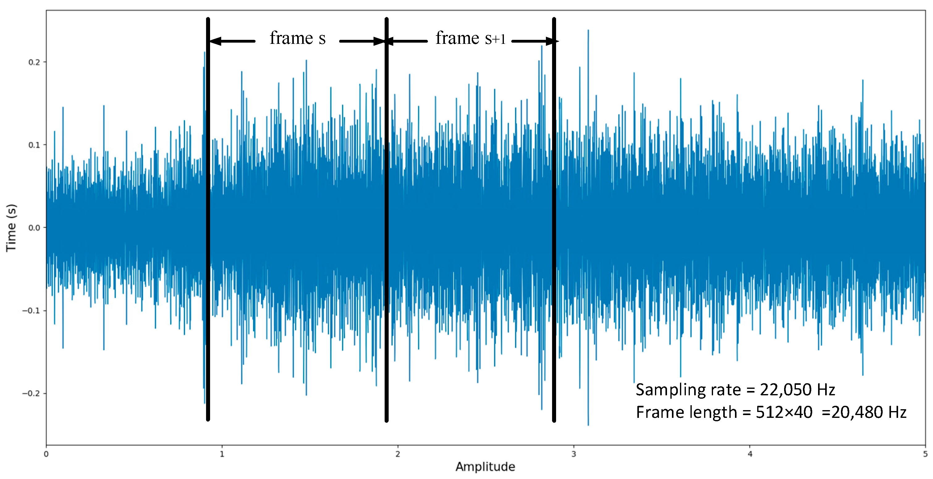
2.1. Preprocessing
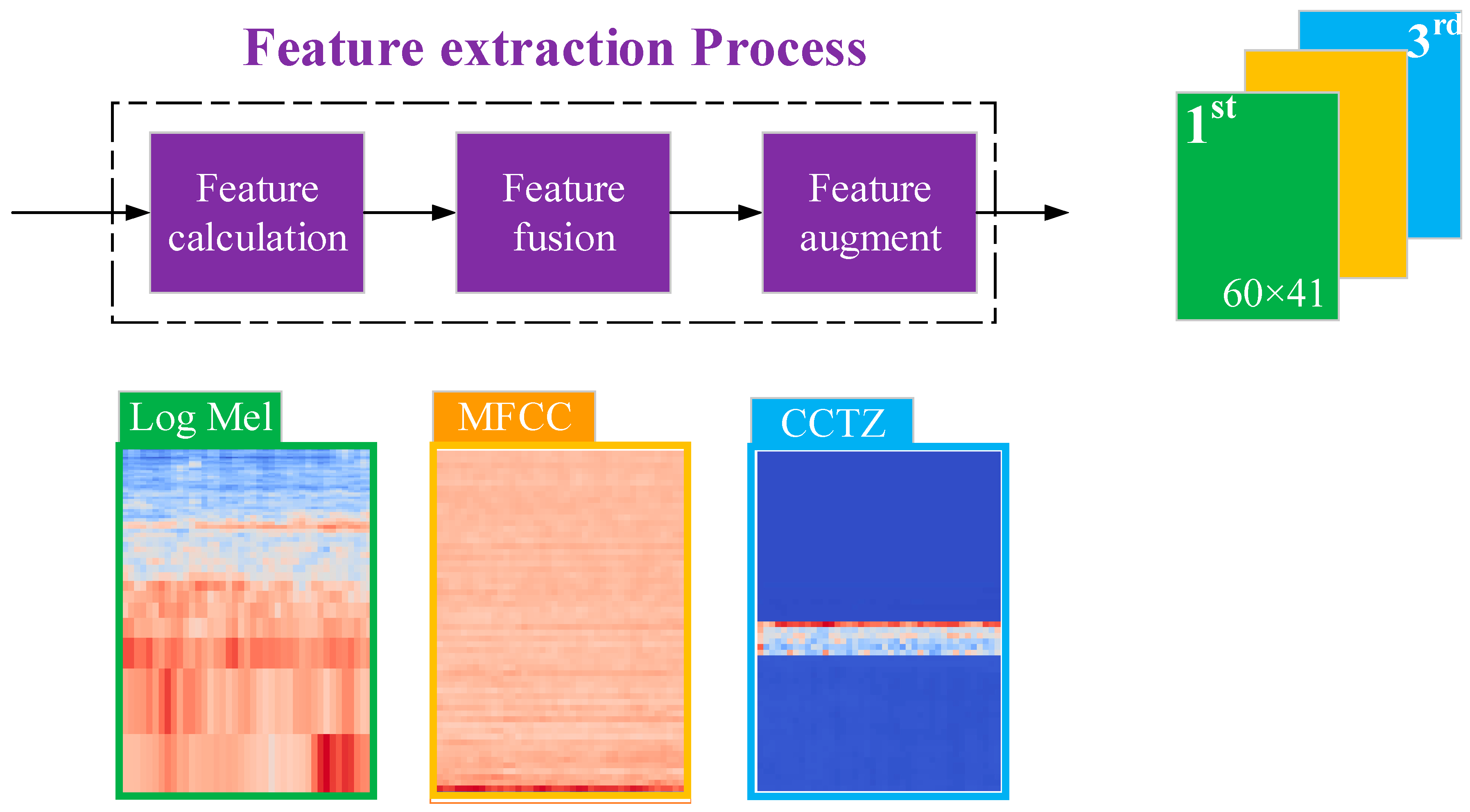
2.2. Feature Extraction Process
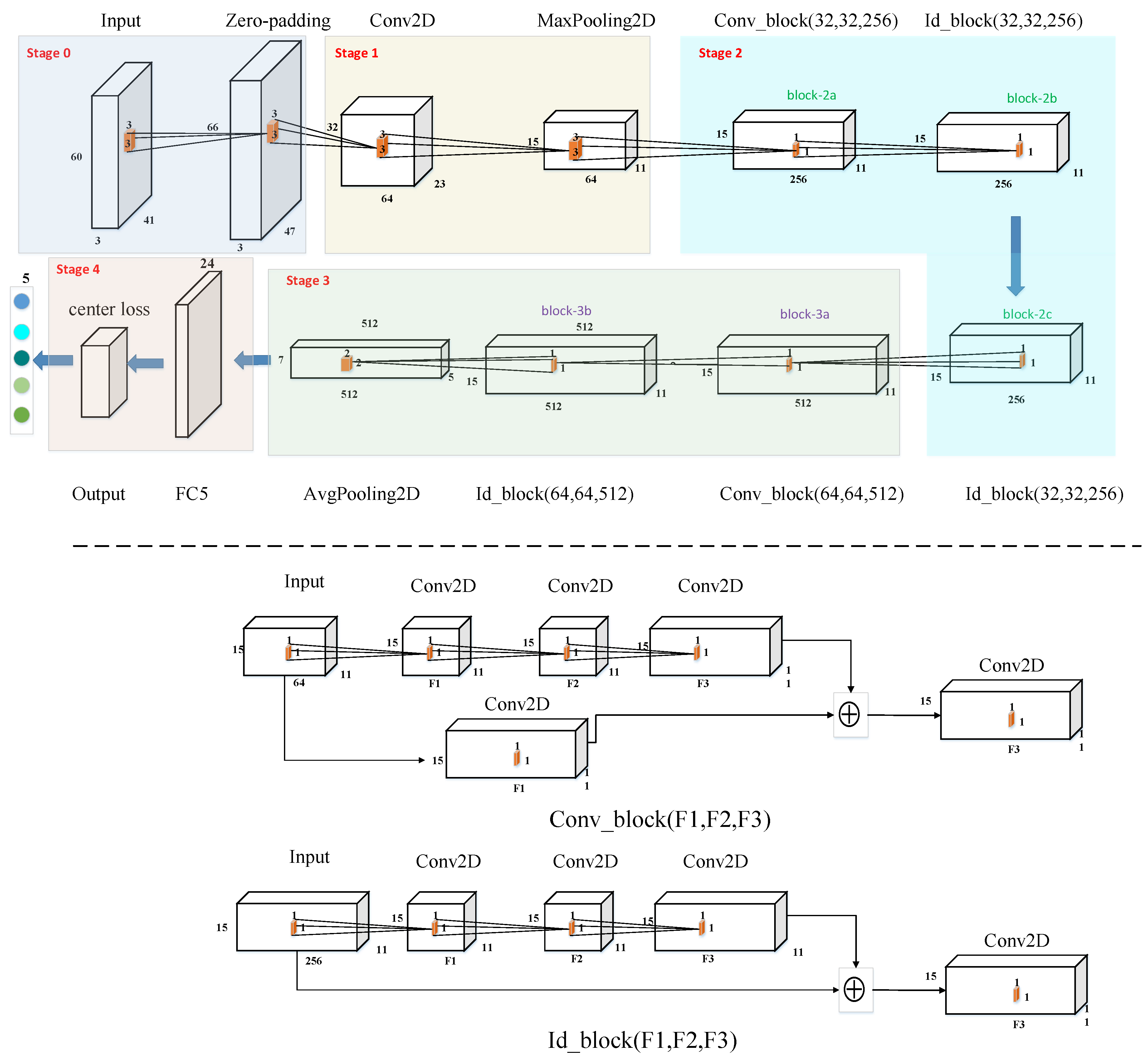
2.3. Structure of the ResNet18
- Stage 0: The input layer is zero-paddled of 3 × 3. After the processing, the shape changes from 60 × 41 × 3 to 66 × 47 × 3.
- Stage 1: The first stage consists of a convolutional layer of 64 filters of the rectangular shape of 3 × 3 and stride of 2 × 2. The batch-normalization is applied, followed by a Rectified Linear Unit (ReLU) as the activation function and max-pooling of 3 × 3 and a stride of 2 × 2.
- Stage 2: The second stage consists of a convolutional block named “block-2a,” an identity block named “block-2b,” and an identity block named “block-2c.” The structure of the convolutional block and the identity block is shown as Conv_block and Id_block in Figure 4, respectively.
- Stage 3: The third stage consists of a convolutional block named “block-3a,” an identity block named “block-3b,” and the average pooling layer of 2 × 2. After processing, the shape of the output of the flatten layer changes from 15 × 11 × 512 to 7 × 5 × 512.
- Stage 4: The stage contains the flatten layer and the designed module of center loss. The number of hidden units of the first fully connected layer is 17,920. As for the designed module of center loss, the second fully connected layer with 24 hidden units connects to the first layer, followed by the Parametric Rectified Linear Unit (PReLU) as the activation function. The last fully connected is with 5 hidden units.
2.4. The Embedding Layer with the Center Loss Function and Softmax
3. Experiments and Analysis
3.1. Dataset Description and Preparation
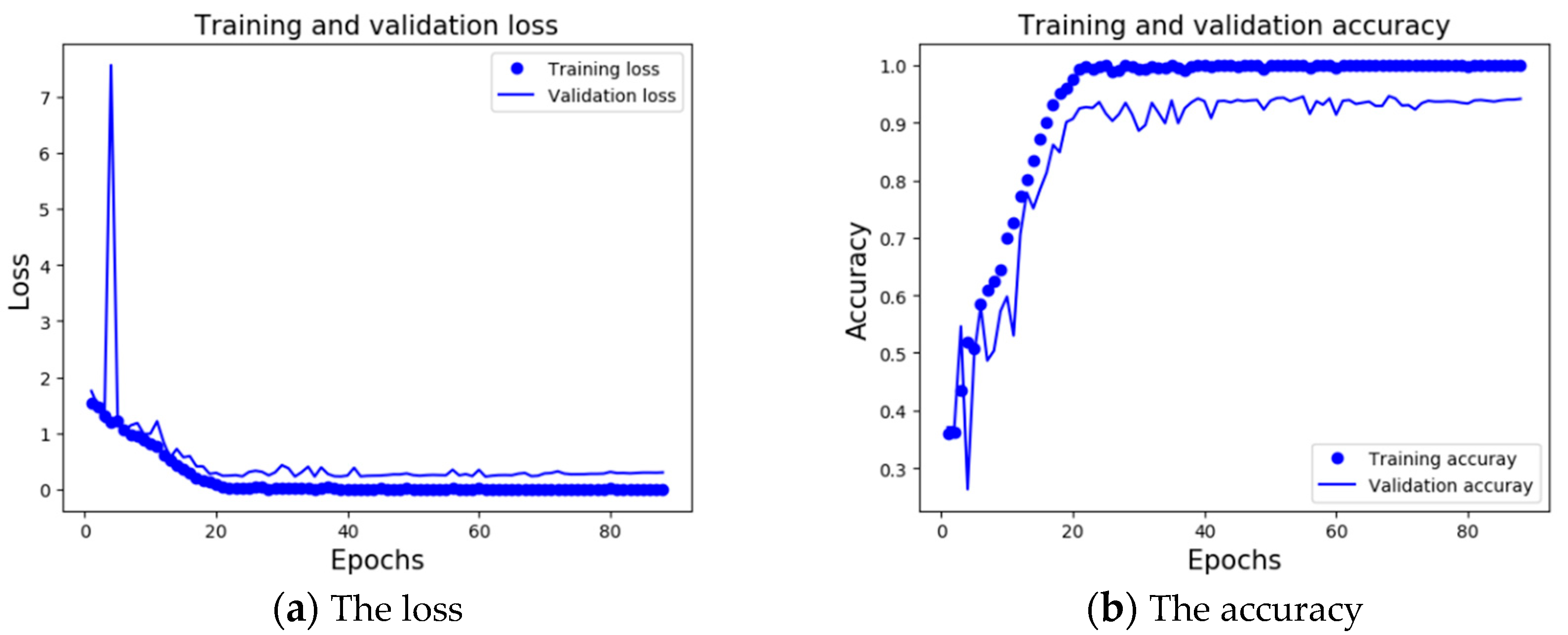
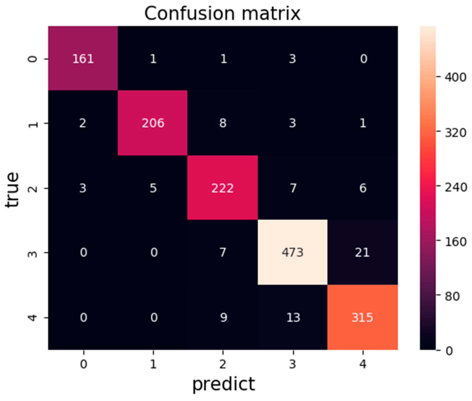
3.2. Experimental Result
3.3. Experimental Analysis
3.3.1. Experiment A: The Advantage of the Feature Extraction Method
3.3.2. Experiment B: The Advantage of the ResNet18 Model
3.3.3. Experiment C: The Contribution of the Embedding Layer with the Center Loss Function and Softmax
4. Conclusions
Author Contributions
Funding
Institutional Review Board Statement
Informed Consent Statement
Data Availability Statement
Conflicts of Interest
References
- Chen, C.; Fu, J. Recognition method of underwater target radiated noise based on convolutional neural network. Acoust. Technol. 2019, 38, 424. [Google Scholar]
- Pezeshki, A.; Azimi-Sadjadi, M.R.; Scharf, L.L.; Robinson, M. Underwater target classification using canonical correlations. In Proceedings of the Oceans Celebrating Past Teaming Toward Future, San Diego, CA, USA, 22–26 September 2003; pp. 1906–1911. [Google Scholar]
- Pezeshki, A.; Azimi-Sadjadi, M.R.; Scharf, L.L. Undersea target classification using canonical correlation analysis. IEEE J. Ocean. Eng. 2007, 32, 948–955. [Google Scholar] [CrossRef][Green Version]
- Ke, X.; Yuan, F.; Cheng, E. Underwater Acoustic Target Recognition Based on Supervised Feature-Separation Algorithm. Sensors 2018, 18, 4318. [Google Scholar] [CrossRef] [PubMed]
- Li, C.; Liu, Z.; Ren, J.; Wang, W.; Xu, J. A Feature Optimization Approach Based on Inter-Class and Intra-Class Distance for Ship Type Classification. Sensors 2020, 20, 5429. [Google Scholar] [CrossRef] [PubMed]
- Meng, Q.; Yang, S.; Piao, S. The classification of underwater acoustic target signals based on wave structure and support vector machine. J. Acoust. Soc. Am. 2014, 136, 2265. [Google Scholar] [CrossRef]
- Jian, L.; Yang, H.; Zhong, L.; Ying, X. Underwater target recognition based on line spectrum and support vector machine. In Proceedings of the International Conference on Mechatronics, Control and Electronic Engineering (MCE2014), Shenyang, China, 29–31 August 2014; Atlantis Press: Paris, France, 2014; pp. 79–84. [Google Scholar]
- Zhang, L.; Wu, D.; Han, X.; Zhu, Z. Feature extraction of underwater target signal using Mel frequency cepstrum coefficients based on acoustic vector sensor. J. Sens. 2016, 2016, 7864213. [Google Scholar] [CrossRef]
- Zhang, Z.; Xu, S.; Cao, S.; Zhang, S. Deep Convolutional Neural Network with Mixup for Environmental Sound Classification. arXiv 2018, arXiv:1808.08405. [Google Scholar]
- Li, J.; Dai, W.; Metze, F.; Qu, S.; Das, S. A comparison of deep learning methods for environmental sound detection. In Proceedings of the 2017 IEEE International Conference on Acoustics, Speech and Signal Processing (ICASSP), New Orleans, LA, USA, 5–9 March 2017; pp. 126–130. [Google Scholar]
- Su, Y.; Zhang, K.; Wang, J.; Madani, K. Environment Sound Classification Using a Two-Stream CNN Based on Decision-Level Fusion. Sensors 2019, 19, 1733. [Google Scholar] [CrossRef] [PubMed]
- Hu, G.; Wang, K.; Peng, Y.; Qiu, M.; Shi, J.; Liu, L. Deep learning methods for underwater target feature extraction and recognition. Comput. Intell. Neurosci. 2018, 2018, 1214301. [Google Scholar] [CrossRef] [PubMed]
- Testolin, A.; Diamant, R. Combining Denoising Autoencoders and Dynamic Programming for Acoustic Detection and Tracking of Underwater Moving Targets. Sensors 2020, 20, 2945. [Google Scholar] [CrossRef] [PubMed]
- Testolin, A.; Kipnis, D.; Diamant, R. Detecting Submerged Objects Using Active Acoustics and Deep Neural Networks: A Test Case for Pelagic Fish. IEEE Trans. Mob. Comput. 2020. [Google Scholar] [CrossRef]
- Shen, S.; Yang, H.; Li, J.; Xu, G.; Sheng, M. Auditory Inspired Convolutional Neural Networks for Ship Type Classification with Raw Hydrophone Data. Entropy 2018, 20, 990. [Google Scholar] [CrossRef] [PubMed]
- Santos-Domínguez, D.; Torres-Guijarro, S.; Cardenal-López, A.; Pena-Gimenez, A. ShipsEar: An underwater vessel noise database. Appl. Acoust. 2016, 113, 64–69. [Google Scholar] [CrossRef]
- Yang, H.; Shen, S.; Yao, X.; Sheng, M.; Wang, C. Competitive deep-belief networks for underwater acoustic target recognition. Sensors 2018, 18, 952. [Google Scholar] [CrossRef] [PubMed]
- Luo, X.; Feng, Y. An Underwater Acoustic Target Recognition Method Based on Restricted Boltzmann Machine. Sensors 2020, 20, 5399. [Google Scholar] [CrossRef] [PubMed]
- Abdoli, S.; Cardinal, P.; Lameiras Koerich, A. End-to-end environmental sound classification using a 1D convolutional neural network. Expert Syst. Appl. 2019, 136, 252–263. [Google Scholar] [CrossRef]
- Park, D.S.; Chan, W.; Zhang, Y.; Chiu, C.C.; Zoph, B.; Cubuk, E.D.; Le, Q.V. SpecAugment: A Simple Data Augmentation Method for Automatic Speech Recognition. arXiv 2019, arXiv:1904.08779. [Google Scholar]
- He, K.; Zhang, X.; Ren, S. Deep Residual Learning for Image Recognition. In Proceedings of the IEEE Conference on Computer Vision & Pattern Recognition, Las Vegas, NV, USA, 27–30 June 2016. [Google Scholar]
- Wen, Y.; Zhang, K.; Li, Z.; Qiao, Y. A discriminative feature learning approach for deep face recognition. In ECCV; Springer: Cham, Switzerland, 2016; pp. 499–515. [Google Scholar]


| Class A | Class B | Class C | Class D | Class E |
|---|---|---|---|---|
| Background noise | Fishing boats, trawlers, mussel boats, tugboats, and the dredger | Motorboats, pilot boats, and sailboats | Passenger ferries | Ocean liners and ro-ro vessels |
| Precision | Recall | F1-Score | Support | |
|---|---|---|---|---|
| Class A | 0.970 | 0.958 | 0.964 | 166 |
| Class B | 0.958 | 0.936 | 0.947 | 220 |
| Class C | 0.917 | 0.914 | 0.915 | 243 |
| Class D | 0.945 | 0.956 | 0.950 | 501 |
| Class E | 0.935 | 0.941 | 0.938 | 337 |
| Average | 0.943 | 0.943 | 0.943 | 1467 |
| MFCC | MFCC + Δ + Δ2 | LM | LM + MFCC | LM + MFCC + CTZZ | |
|---|---|---|---|---|---|
| Class A | 0.955 | 0.982 | 0.966 | 0.967 | 0.964 |
| Class B | 0.821 | 0.844 | 0.914 | 0.899 | 0.947 |
| Class C | 0.792 | 0.821 | 0.851 | 0.840 | 0.915 |
| Class D | 0.924 | 0.919 | 0.913 | 0.934 | 0.950 |
| Class E | 0.898 | 0.845 | 0.900 | 0.907 | 0.938 |
| Average | 0.884 | 0.882 | 0.906 | 0.911 | 0.943 |
| Model | CNN-1 | CNN-2 | LSTM | CRNN | ResNet18 |
|---|---|---|---|---|---|
| Feature | MFCC | LM + MFCC + CCTZ | LM | LM + MFCC + CCTZ | LM + MFCC + CCTZ |
| Class A | 0.926 | 0.973 | 0.831 | 0.936 | 0.964 |
| Class B | 0.806 | 0.902 | 0.805 | 0.867 | 0.947 |
| Class C | 0.744 | 0.853 | 0.869 | 0.832 | 0.915 |
| Class D | 0.881 | 0.919 | 0.862 | 0.908 | 0.950 |
| Class E | 0.832 | 0.897 | 0.875 | 0.876 | 0.938 |
| Average | 0.845 | 0.906 | 0.852 | 0.885 | 0.943 |
| Model | Accuracy |
|---|---|
| Baseline [15] | 0.754 |
| RBM + BP [14] | 0.932 |
| RSSD [4] | 0.933 |
| ResNet18 + 3D | 0.943 |
| Model | ResNet18 | ResNet18 | ResNet18 |
|---|---|---|---|
| Feature | LM + MFCC + CCTZ | LM + MFCC + CCTZ | LM + MFCC + CCTZ |
| Loss function | Softmax | Uniform loss | Center loss |
| Class A | 0.967 | 0.979 | 0.964 |
| Class B | 0.892 | 0.938 | 0.947 |
| Class C | 0.874 | 0.894 | 0.915 |
| Class D | 0.922 | 0.945 | 0.950 |
| Class E | 0.923 | 0.924 | 0.938 |
| Average | 0.910 | 0.934 | 0.943 |
Publisher’s Note: MDPI stays neutral with regard to jurisdictional claims in published maps and institutional affiliations. |
© 2021 by the authors. Licensee MDPI, Basel, Switzerland. This article is an open access article distributed under the terms and conditions of the Creative Commons Attribution (CC BY) license (http://creativecommons.org/licenses/by/4.0/).
Share and Cite
Hong, F.; Liu, C.; Guo, L.; Chen, F.; Feng, H. Underwater Acoustic Target Recognition with a Residual Network and the Optimized Feature Extraction Method. Appl. Sci. 2021, 11, 1442. https://doi.org/10.3390/app11041442
Hong F, Liu C, Guo L, Chen F, Feng H. Underwater Acoustic Target Recognition with a Residual Network and the Optimized Feature Extraction Method. Applied Sciences. 2021; 11(4):1442. https://doi.org/10.3390/app11041442
Chicago/Turabian StyleHong, Feng, Chengwei Liu, Lijuan Guo, Feng Chen, and Haihong Feng. 2021. "Underwater Acoustic Target Recognition with a Residual Network and the Optimized Feature Extraction Method" Applied Sciences 11, no. 4: 1442. https://doi.org/10.3390/app11041442
APA StyleHong, F., Liu, C., Guo, L., Chen, F., & Feng, H. (2021). Underwater Acoustic Target Recognition with a Residual Network and the Optimized Feature Extraction Method. Applied Sciences, 11(4), 1442. https://doi.org/10.3390/app11041442