Abstract
The measurement of reverberation time is an essential procedure for the characterization of the acoustic performance of rooms. The values returned by these measurements allow us to predict how the sound will be transformed by the walls and furnishings of the rooms. The measurement of the reverberation time is not an easy procedure to carry out and requires the use of a space in an exclusive way. In fact, it is necessary to use instruments that reproduce a sound source and instruments for recording the response of the space. In this work, an automatic procedure for estimating the reverberation time based on the use of artificial neural networks was developed. Previously selected sounds were played, and joint sound recordings were made. The recorded sounds were processed with the extraction of characteristics, then they were labeled by associating to each sound the value of the reverberation time in octave bands of that specific room. The obtained dataset was used as input for the training of an algorithm based on artificial neural networks. The results returned by the predictive model suggest using this methodology to estimate the reverberation time of any closed space, using simple audio recordings without having to perform standard measurements or calculate the integration explicitly.
1. Introduction
The sound field in a physically confined environment differs from that of an open space due to the presence, next to the direct sound waves between source and receiver, of sound waves reflected in various ways from the surrounding surfaces. The elements present inside an enclosed space, be they walls, furniture and people, influence the acoustic propagation by absorbing a part of the incident sound energy. The first wave front emitted by any source that reaches the receiver is called direct sound: it has not undergone absorption or reflection. The successive wave fronts constitute the reverberant field and are due to the complex of interactions that the sound wave undergoes due to the surfaces that delimit the space or to the objects it contains. Direct sound prevails near the source, while reverberant sounds prevail at a distance [1,2].
The direct wave behaves in a similar way to the propagation of sound in a free field, it decays by simple geometric divergence, with an acoustic intensity inversely proportional to the square of the distance from the source. This wave is simultaneously integrated by the first reflections coming from the surrounding surfaces. For the reverberated sound, the first reflections are distinguished, which reach the listener within a few tens of milliseconds after the direct sound from subsequent reflections which are masking. The total sound field is therefore given by the combination of the direct sound field and the reverberant field. The optimal combination of the two fields varies according to the type of sound signal to be transmitted in the room [3,4].
To address these issues, different methodologies can be used. The simpler approach, called geometric acoustics, is based on the study of the path of the sound rays that are gradually reflected by the surfaces delimiting the space, in the simplified hypothesis of specular reflection. A more rigorous approach, on the other hand, analyzes the propagation of sounds from the wave point of view, considering the space as a complex system where many standing waves of different wavelengths, called vibration modes, can coexist. In general, when the dimensions of the space are comparable to the wavelengths of sound waves, a rigorous analysis cannot be ignored [5,6].
The acoustic quality of confined spaces has been the subject of considerable attention for years, even if a single procedure for their design has not yet been reached. Investigations carried out by statistically elaborating subjective judgments of many listeners have shown that, beyond the subjective evaluations, there are some objective parameters of the acoustic field capable of acoustically characterizing the spaces. Over the years, numerous scholars have proposed various methods of determining these parameters, assigning each of them a different weight [7,8,9,10,11].
The first example in this sense was given by Sabine [12], at the beginning of the last century, that identified the reverberation time as a fundamental parameter, and studied its optimal values for the various types of music and provided a simple relationship for its calculation. The reverberation time was the main, if not the only, physical descriptor used as an objective parameter for evaluating the acoustic behavior of a room until the 1950s. A single value, for each frequency band, can be representative of the sound field of the entire room only if this is sufficiently reverberant (where the average absorption coefficient is less of 0.25 [13]) and if it is homogeneously so, otherwise a value should be calculated at each listening point. The reverberation time indicates the time, in seconds, required so that, in a defined position, in a confined space, the sound level is reduced by a defined amount compared to what it had in the instant prior to the interruption of the sound source [14].
The measurement of the reverberation time is not an easy procedure to carry out and requires the use of a space in an exclusive way. In fact, it is necessary to use instruments that reproduce a sound source and instruments for recording the response of the space. In this work, an automatic procedure for estimating the reverberation time based on the use of artificial neural networks was developed. Section 2 presents the methodologies used to measure the reverberation times of the rooms under analysis, as well as the procedures for selecting and recording the sample sounds. The architecture of the algorithm based on the artificial neural networks used is also presented. In Section 3 the results obtained in this study are presented and adequately discussed. Finally, Section 4 summarizes the objectives of this study and the results obtained.
2. Materials and Methods
2.1. Reverberation Time
Reverberation time is a key parameter when it comes to acoustics in confined spaces. This is the decay of the sound following the switching off of a source and due to the sound reflections, that continue to travel in the space. The sound energy that affects a surface S is divided into three components: a part is reflected by the surface, a part is absorbed, and a part transmitted beyond the material [15,16,17].
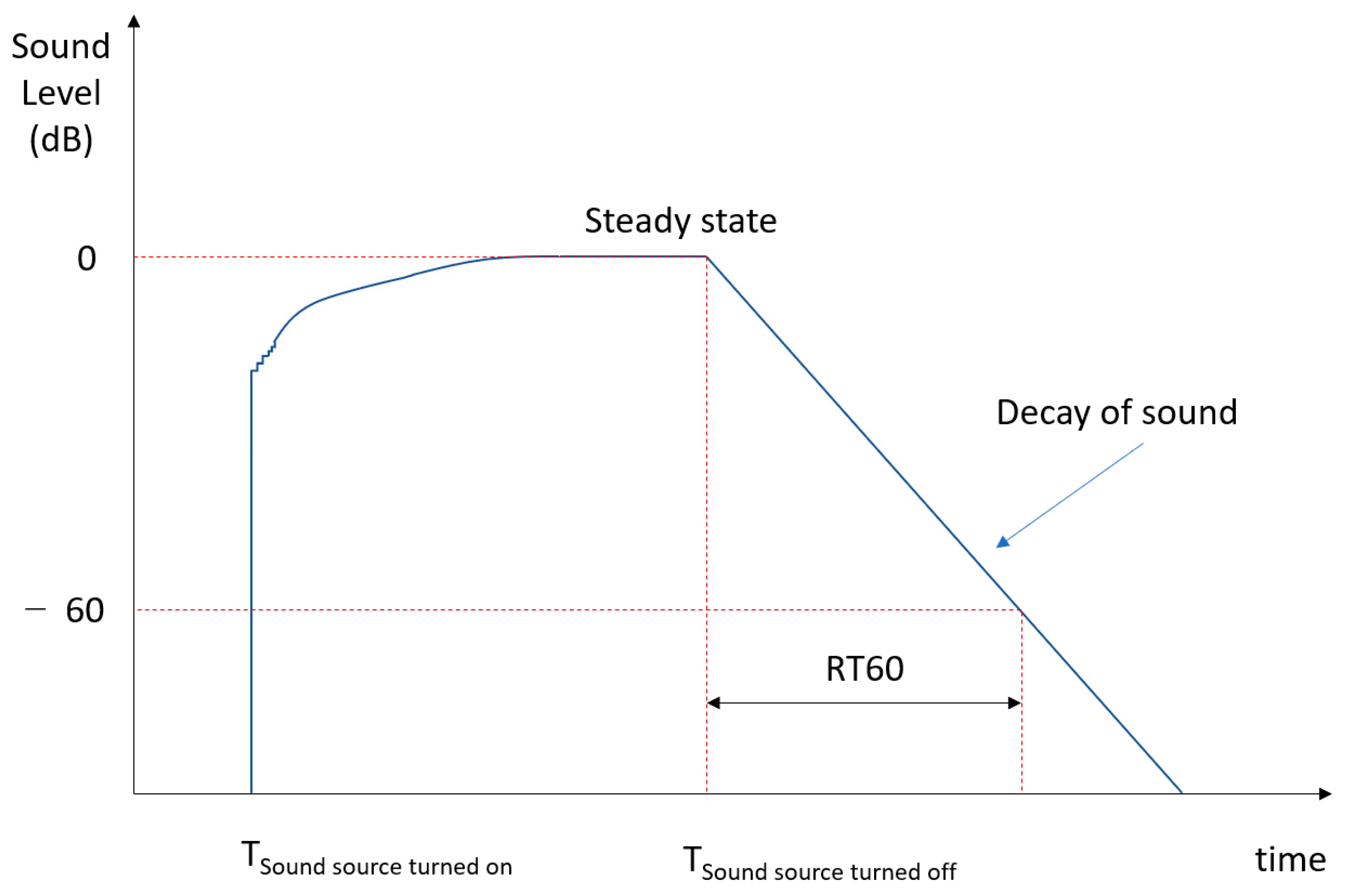
Before the sound emitted from a generic source reaches the receiver, a time, called the sound wave propagation time, passes, equal to the ratio between the distance of the source from the receiver and the speed of sound. The receiver will receive various contributions deriving from the source, those related to direct sound and those due to reflections. Clement W. Sabine defined this parameter at the end of the 1800s as: given an interrupted stationary source, the reverberation time is the time between the instant in which the direct sound ends and the instant in which the sound level has dropped by 60 dB [18], as shown in Figure 1. In a room, the longer the reverberation time, the greater the contribution of the components of the reflected sound compared to the direct one. The absorption of the materials changes with the frequency, so the reverberation time also varies at the different frequencies considered. In architectural acoustics the frequencies in the octave bands from 125 to 4000 Hz are considered. Frequencies above 4000 Hz are not considered because sound absorption by air prevails. Frequencies below 125 Hz are not considered because the human ear has a reduced sensitivity at low frequencies.
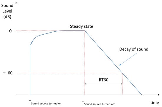
Figure 1.
Diagram for the evaluation of the reverberation time (RT60) using the natural decay curve of a sound signal. Reverberation time is the time between the instant in which the direct sound ends and the instant in which the sound level has dropped by 60 dB.
Sabine, through a series of experiments, found that the value of this parameter (RT60) depended on the volume of the space and the total absorption of its internal surfaces. With the same shape of the confined space, the reverberation time increases linearly as the size increases. According to Sabine, the reverberation time value is a function of the room volume and the total sound absorption of its internal surfaces [18] as descripted in the following equation:
Here:
- T60 is the time in seconds required for a sound to decay 60 dB
- 0.161 is a dimensioned factor (s/m)
- V is the volume of the room in m3
- is the i-th sound absorption coefficient
- Si is the i-th surface in m2 with a
The sound absorption coefficient is a number that varies between 0 and 1:0 indicates absence of absorption, that is the surface is totally reflective, while 1 indicates total absorption without reflection. The sound absorption coefficient is used to evaluate the sound absorption efficiency of the materials. It is defined as the ratio of absorbed energy to incident energy. The measurement techniques of this parameter are essentially two for normal and random incidence. The measurement of the sound absorption coefficient for normal incidence is performed in a Kundt tube in accordance with ISO 10534 [19] to know the percentage of sound absorbed by a material. It is the only test in which there is no margin of discretion in the setup phase, since it is a sample of material inserted into a tube and hit by a direct wave. The measurement of the sound absorption coefficient for random incidence is performed in a reverberation room in accordance with ISO 354 [20] to calculate the percentage of sound absorbed by a product hit by waves from various directions, simulating a situation of real use. The test setup can affect the result since the absorption of a panel also depends on its position within a room such as the distance from rigid surfaces and the distance between panels.
The reverberation of a space has positive and negative aspects: in fact, if a certain value of the reverberation time helps to reinforce the direct sound it therefore improves listening; on the other hand, an excessive value of the sound tail compromises its quality [1,2]. For good reception, both in the case of speech and in the case of music, it is necessary to contain the decaying tail of reflected sound from a source and ensure a good spatial distribution of the sound field inside the room so that all listeners can perceive and appreciate the sound regardless of the space in which they are located [21].
An optimal reverberation time represents the right compromise between achieving a sufficient sound level in all parts of the space and reducing blending and overlap with reflected sounds caused by excess reverberation [22]. So, the optimal value of the reverberation time depends on the use to which the space is intended (Table 1). In Table 1 the parameters are defined as follows:

Table 1.
Optimal reverberation time values for different listening conditions [6].
- • T30 is a measure of reverberation time using a 30 dB interval with the evaluation starting after the sound level has dropped by 5 dB from steady state.
Since the absorption of the materials varies with the frequency, the reverberation time must also be calculated at the various frequencies. The measurement of the reverberation time can be performed according to the ISO 3382-2 [23]. The standard specifies the methods for measuring the reverberation time in rooms. In addition, it describes the measurement process, the equipment required, the coverage required and the method of evaluating the data and submitting the test report. The standard proposes two methods for measuring the reverberation time: the interrupted noise method and the integrated impulse response method. Both methods return comparable values, but the second requires more sophisticated tools [24,25].
In the interrupted noise method, a loudspeaker source must be used, and the input signal must be derived from random or pseudorandom broadband electrical noise. If a pseudo causal noise is used, it must randomly stop without using a repeat sequence. The sound source should be as omnidirectional as possible. The number of microphone stations used is determined by the coverage requested. Given the intrinsic randomness of the sound source, it is necessary to average over several measurements performed at each station to obtain an acceptable repeatability. Therefore, a minimum of three measurements should be made at each position and the results averaged.
The impulse response from a source position to a receiver position in an environment is a well-defined quantity that can be measured in many ways, using for example gunshots, firecrackers, or hand claps as signals. The pulse source must be able to produce a peak sound pressure level sufficient to ensure a decay curve that begins at least 45 dB greater than the background noise in the corresponding frequency band [26].
2.2. Acoustic Measurements
The acoustic measurements were carried out in empty rooms without people with an average internal temperature of about 20 °C and a relative humidity of 50%. There were no noisy activities in the vicinity, and the noise of vehicular traffic was negligible considering the distance from the nearest road. To further reduce the background noise, the measurements were carried out without any persons, so the impulse responses were all recorded under empty conditions. During the acoustic measurements, the background sound level was less than 35 dB.
To collect the data necessary for the training of the predicting model, acoustic measurements were carried out in the rooms chosen for this study. Two types of measurements were made: sound recordings of the room response to the reproduced sounds, and impulse response measurements for the evaluation of the reverberation time.
Sound recordings of the room’s response to the reproduced sounds were performed with a high-quality portable recorder Zoom H6 Handy Recorder (Zoom Corporation, Tokyo, Japan) with a X–Y microphone (Table 2). The sounds sampled for the measurement of the room response were reproduced with a Bluetooth speaker (Table 2).

Table 2.
Recording and reproducing sound instrument specifications.
To ensure an adequate ability to generalize to the prediction model, ten sounds of different types were selected. The choice of sounds was made to cover all the frequencies of the audible spectrum (20 Hz–20 kHz), favoring sounds with content in specific and diversified frequency ranges.
The measurement of the reverberation time of the rooms is simply aimed at obtaining the value necessary to label the data to be used as input to the prediction model. For the measurement of the reverberation time the integrated impulse response method [23] was adopted. Toy balloons inflated with air were used as the sound source to produce the impulsive sound. This impulsive source has already been used in previous studies [27], the burst of a balloon produces an impulse that excites the sound field, furthermore the background noise is very low as it is far from anthropogenic noises. The bursting of a balloon provides a sufficient SNR ratio. Signal-to-noise ratio (SNR) is a measure that compares the level of a desired signal to the level of background noise.
Ten equally distributed recording points were identified for the evaluation of the spatial average of the acoustic properties of the room, in each point the device for recording the response of the room was placed. The balloons were popped to a height of 1.6 m from the floor approximately equal to that of the speaker’s mouth, in the position where the speaker’s seat was. The recorder, on the other hand, was positioned in correspondence with the seats, at a height of 0.8 m, to simulate the position of the listeners as much as possible. The recorded impulse responses were subsequently processed with Dirac 4.0 software for the extraction of reverberation time (Schroeder’s backward integration).
2.3. Reverberation Time Prediction Methodology Based on Artificial Neural Network
To simplify the procedure for estimating the reverberation time of a room, a methodology based on the use of artificial neural networks was studied. Mathematically, the topology of an artificial neural network defines a space of hypothesis, also called the space of possibilities, in which useful representations of the data to be analyzed can be sought.
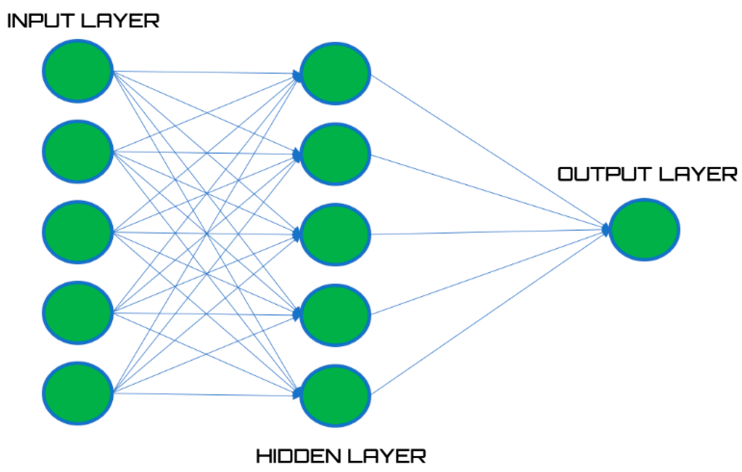
A generic multilayer network is represented by a succession of layers (Figure 2): the first layer is called the input layer, the outputs of which are supplied in input to the subsequent layers which are called hidden layers. The adjective “hidden” derives from the fact that, in these levels, the representation of the data is transitory, and as a result hidden from the outside world, therefore we cannot properly speak of output values for them. The last layer of the network is called the output layer and contains from 1 to N neurons whose task is to provide the real network output based on the required task [28].
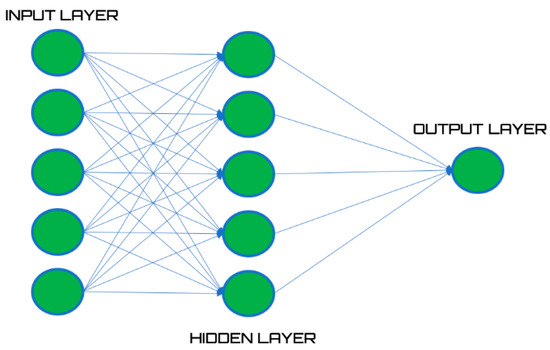
Figure 2.
Artificial neural network architecture.
Each layer is made up of a series of neurons. Information is stored inside each neuron and is transferred to those of the subsequent layers through a connection to which a weight is associated. Weights adjustment represents the real learning task of the entire process and takes place through an adaptation procedure based on an iterative optimization process [29].
Given a set of independent input variables x = (x1, ..., xn), we can define with W the weights matrix, in which each element wji represents the weight of the connection between the i-th node of the input layer and j-th node of the hidden layer. Each row of the weight matrix defines the weights for a single hidden layer node, so the association between the input vector and the output of each hidden node can be illustrated through the following equation:
In Equation (2) the terms are defined as follows:
- hj is the j-th output of the hidden layer
- f is the activation function
- is an element of the weight matrix
- xi is the i-th input
- b is the bias
An essential feature of this technology is the activation function: Its importance lies in the fact that a neural network without an activation function essentially behaves like a normal regression model whose purpose is to provide a function that best approximates the provided data input and that, at the same time, is flexible enough to allow a forecast of a possible output value. Initially, in the history of neural network-based algorithms implementation, the first network structures were designed to perform purely linear logical operations, the function that was to approximate the input points was therefore linear [30]. With the evolution of networks, this linear function represented the distribution of points in an imprecise way. For this reason, it was decided to introduce, within the networks, an element of non-linearity, hence the sigmoidal activation function.
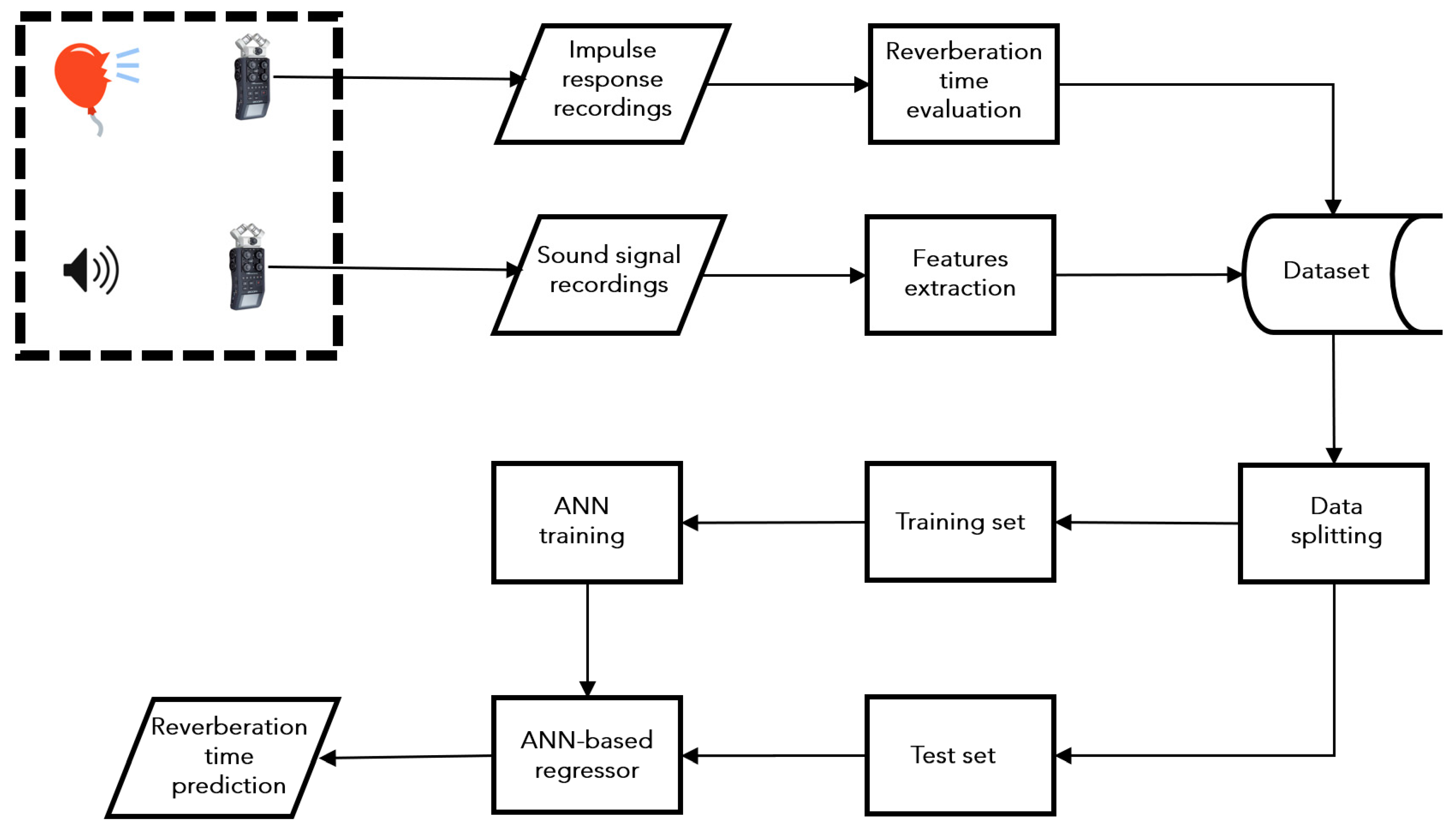
The developed methodology aims to predict the value of the reverberation time, based on recordings of the responses of a room to a series of signals. To train the network, recordings were made in a series of rooms characterized by different reverberation times. This methodology is based on the following steps (Figure 3):
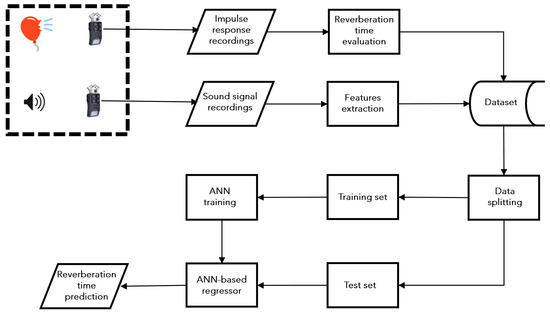
Figure 3.
Flow chart for the reverberation time prediction methodology based on artificial neural network. Two sound recordings are made: the first to record the impulse response of the room to calculate the reverberation time. This value will be used in the training phase to label values. The second recording will be used to estimate the reverberation time of the room using a method based on a supervised learning algorithm.
- Reverberation time measurement using the integrated impulse response method.
- Recordings of a series of signals.
- Features extraction of the recorded signals.
- Construction of a dataset containing the processed data.
- Training of a regression algorithm based on artificial neural networks.
- Regressor test.
Once the prediction system has been set up it will only be necessary to record a signal in a room to derive the reverberation time.
2.4. Feature Extraction
Sound signals are the result of processes occurring in the time domain; however, it is convenient to study them in the frequency domain, both in deterministic and stochastic cases, which is why it is necessary to obtain the power spectral density (PSD) function. The input signal is time-limited, non-stationary and has overlap noise, so PSD needs to be estimated from a record of a certain amount of data. The first methods for PSD estimation were based on the estimation of the Fourier transform (FT). An important step in modern spectral estimation was the work of Wiener [31,32], who established the theoretical basis for the treatment of stochastic processes. Khinchin showed that FT relates the autocorrelation function of a stationary process and its PSD [33]. It is generally called the Wiener–Khinchin theorem. Before the introduction of the fast Fourier transform (FFT) algorithm in 1965, the usual method for estimating PSD was the implementation of the Wiener–Khinchin theorem suggested by Blackman and Tukey [34].
According to this method, the autocorrelation coefficients are estimated using a sequence of event data. To obtain the PSD, the Fourier transform of this window correlation is performed. This method is often also called the indirect method. Since the introduction of the FFT, which implied the provision of a computationally efficient algorithm for the computation of the discrete Fourier transform (DFT), the direct approximation (periodogram) is used intensively, which is obtained as a square quantity of the obtained DFT by FFT and applied directly to the data.
The power spectrum (PS) is defined as the Fourier transform of the autocorrelation function, as in the following Equation (3):
In Equation (3) rxx is the autocorrelation function as defined in the Equation (4).
Here x is the signal. The power spectrum returns the power distribution of a signal over a range of frequencies. The power spectrum can be evaluated by applying the Fourier transform on the entire signal. However, the averaging of the spectra is used, particularly when the available waveform is only a sample of a longer signal. In this case we speak of a periodogram [35].
The periodogram is calculated by dividing the signal into several segments, possibly overlapping, and evaluating the Fourier transform on each of these segments: On two successive data segments a shift of a number of points equal to D is performed. Each segment is made up of N points, where the i-th sequence is given by the following expression:
The overlap between two consecutive segments xi(n) and xi + 1(n) is equal to N-D points. If a 50% overlap is allowed, as proposed by Welch [36], the number of sections K of the length L is calculated using the following equation:
Using Equation (6), the length of the sequence does not vary. Additionally, doubling the number of periodograms to be averaged reduces the variance. The final spectrum is obtained as the average of the different spectra obtained on the segments. The frequency resolution of the spectrum is approximately 1/N, where N is the number of samples per segment. Taking a small segment increases the number of segments to the mean and thus increases the smoothing in the estimated spectrum. At the same time the frequency resolution is reduced. The overlap associated with the periodogram calculated with the Welch method helps to significantly improve the correlation of the data, improving its statistical properties and therefore improving the reliability of the estimate [37].
For discrete-time systems, the Welch periodogram returns an estimate of the power spectral densities. This method segments the time signal into periods of a certain block size. For each period, the spectrum is calculated through an average estimate of the final spectral density. The block size affects the duration of the individual segments and the spectral resolution of the final estimate of the power density.
The PSD extracted from the recorded signals was subsequently used for the estimation of the magnitude-squared coherence. These values were then used as input for the ANN-based model.
To evaluate the differences between two signals, it is possible to use the concept of coherence which represents an ideal property of waves: It allows a stationary interference that is constant in time and space. Two wave sources are perfectly coherent if their frequency and waveform are identical and their phase difference is constant. More generally, coherence describes all the properties of the correlation between physical quantities of multiple waves. So, to evaluate the effects of the room on the sound field we can use the coherence between the recorded signals (using the Zoom H6 Handy Recorder (Zoom Corporation, Tokyo, Japan) equipped with a X–Y microphone) and the anechoic signal. Coherence is a function of the power spectral densities of the two signals, and of the cross power spectral density [38,39]. Cross-power spectral density is a statistical property of a pair of random sequences that indicates the likely distribution of power over different frequencies at any given time. The cross-power spectral density of a pair of X and Y signals is the Fourier transform of the cross correlation between the signals.
Given two signals a and b, the coherence function is defined by Equation (7):
Here,
- is the cross power spectral density for a and b signals
- is the power spectral density of a signal (coherent signal)
- is the power spectral density of b signal (no-coherent signal = signal modified by the reverberation of the room)
3. Results and Discussions
The first part of the study was used to collect several examples sufficient to train the algorithm effectively. Ten anechoic signals with different characteristics were used to excite the rooms in a different way, to record the response of the rooms to the different sound stresses. An anechoic signal is recorded in an anechoic chamber in which there are no reflections as the walls, the floor and the ceiling absorb all the incident waves. Different sounds with different characteristics were used to ensure an effective generalization capacity for the model.
The characteristics of the signals used are such as to cover all the frequencies of the audible spectrum (20 Hz–20 kHz). Table 3 reports the statistical descriptors of the anechoic signals used in this work [40]. Leq (equivalent continuous sound pressure level) is the constant noise level that would result in the same total sound energy being produced over a given period. Lmax (maximum level) is the noise with maximum energy content. Lmin (minimum level) is the noise with minimum energy content. StdDev is the standard deviation. L95, L90, L50, L10, L5 are the percentile sound levels. The percentile level represents the noise level exceeded for a percentage of the measurement time. For example, L95 represents the noise level exceeded for 95% of the measurement time.

Table 3.
Training signals descriptors in dB.
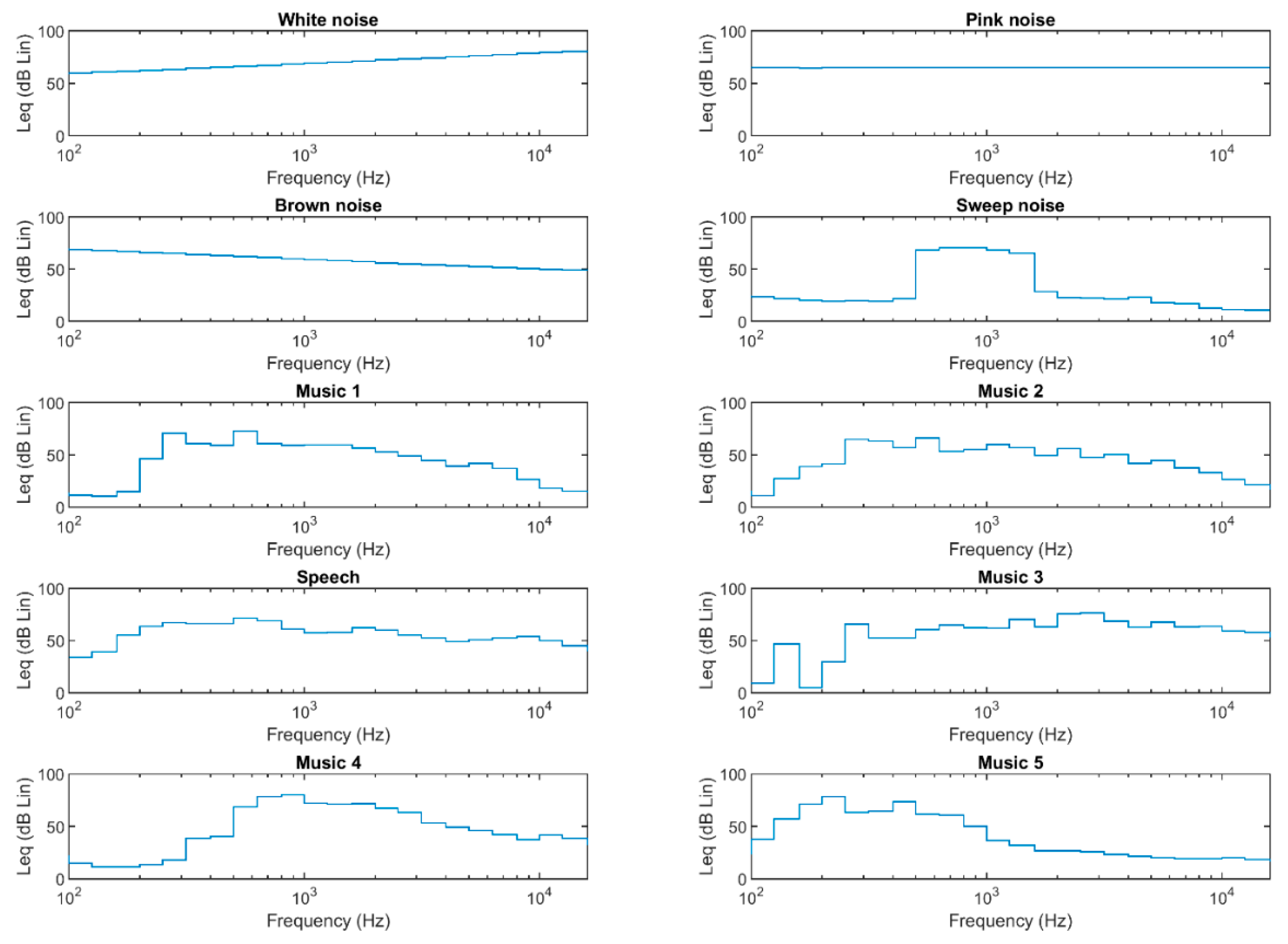
Figure 4 shows the average spectral levels in the one-third octave band between 100 Hz and 16 kHz (dB Lin) for the ten signals used to train and test the models. The first three signals (white noise, pink noise, brown noise) represent artificially generated noise with characteristics that cover the entire frequency spectrum. White noise is characterized by the absence of periodicity and by a constant amplitude that includes all the frequencies of the audible. Pink noise has low frequency components with higher power. Finally, brown noise has an even greater accentuation of the presence of low frequencies than pink noise. The intensity decreases, from one octave to the other, like the inverse of the square of the frequency with an attenuation, on a logarithmic scale, of 6 dB. Sweep noise is a signal composed of a pure tone whose frequency increases over time with a certain trend.
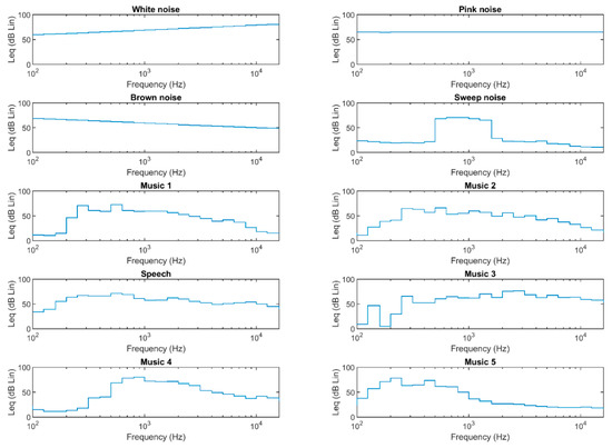
Figure 4.
Average spectral levels in the one-third octave band (dB Lin) between 100 Hz and 16 kHz (logarithm scale) for the ten signals used to train and test the models.
In addition, anechoic female speech and anechoic music signals were used, specifically the music signals concerned various musical instruments with contributions to both low and high frequencies. The diversification of the signals was a choice dictated by a strategy aimed at collecting records that contain the greatest number of information necessary to develop a model capable of generalizing the behavior of the system [41].
The elements present within an enclosed space (walls, furniture, people) affect the acoustic propagation with important effects on the acoustics of the environment itself as they absorb the sound energy that affects them to varying degrees. The acoustics of the room are also conditioned by the size of the room as well as by its geometry. To give the model its ability to generalize the behavior of the system, rooms with different characteristics have been selected both in terms of size, geometry, and furnishings. Twelve rooms with parallelepiped geometry were selected. The rooms are differentiated by volume, by type of flooring, by type of walls, and by type of furniture. Table 4 summarizes the main characteristics of the rooms.

Table 4.
Characteristics of the rooms covered by this study.
Figure 5 shows some of the rooms used in this study. The type of rooms used is diversified: We pass from rooms used as offices, to laboratories, conference rooms, mechanical workshops, and rooms in houses.
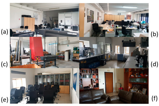
Figure 5.
Example images of some rooms used to record the response of the environment to the sounds played. The rooms have both geometric characteristics and different sizes. The volume of the rooms ranges from approximately 40 m3 to more than 4000 m3. (a) Room 2; (b) Room 1; (c) Room 3; (d) Room 5; (e) Room 4; (f) Room 12.
In each room the reverberation time was measured using the impulse response technique in accordance with ISO 3382 [23]. The rooms were characterized from an acoustic point of view with the values of reverberation time T30. Table 5 shows the octave band reverberation time measured in some of the rooms used in this study.

Table 5.
Reverberation time in the octave band measured in some of the rooms used in this study (s).
As anticipated, the measured reverberation times were used for the construction of the dataset to be used as the input of the prediction model. Using these values, the features extracted from the recordings were appropriately labeled.
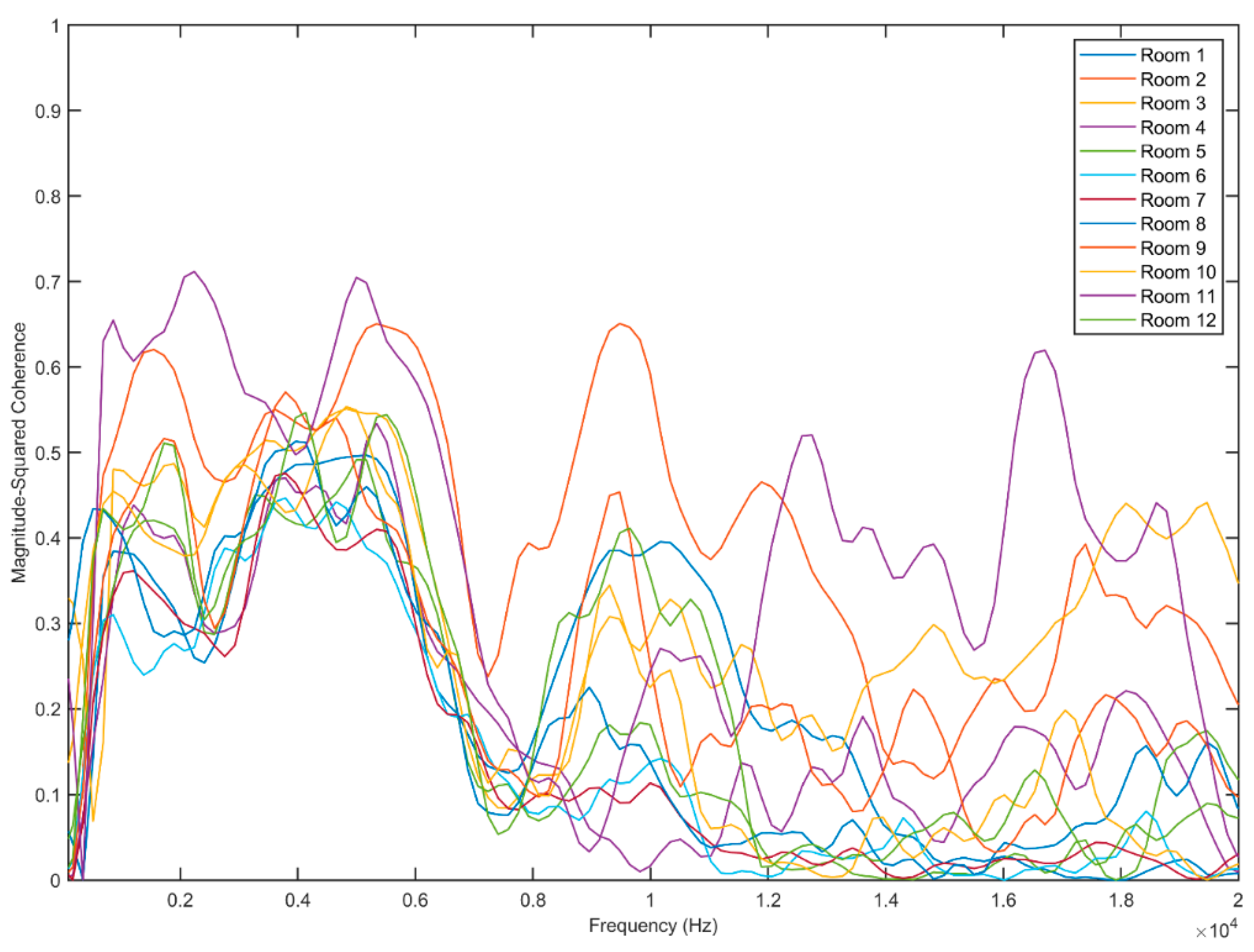
Figure 6 shows the magnitude-squared coherence estimation of the recorded signals in twelve rooms, evaluated using the Equation (7). For each estimation, the same source signal was used (white noise). We can note that the coherence function allows us to discriminate between the different curves and therefore represents an appropriate choice as a descriptor.
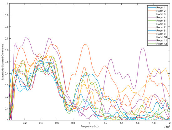
Figure 6.
Magnitude-squared coherence estimation for the signals recorded in twelve rooms. Each curve refers to the same reproduced signal (white noise) and is calculated as function of the power spectral densities, and the cross power spectral density, as reported in Equation (6).
The results returned by a simulation model strongly depends on the quality of the input data that is presented to the algorithm. This is the reason why to obtain a satisfactory result it is necessary to pay particular care and attention to the procedure of processing the input data. In Figure 3 we have presented a flow chart of the entire procedure, in it is possible to notice that the first part of the procedure is aimed at building the dataset that will be used for training the model and subsequently for its validation and testing. We decided to use the spatial coherence function as a characteristic; specifically, the magnitude-squared coherence function as defined in Equation (7) was evaluated. The signals were divided into 100 segments, each segment with a Hamming window of equal bandwidth, in addition a 50% overlap between segments was used. A total of 129 discrete Fourier transform (DFT) points were set, and a frequency range for the estimation of magnitude-squared coherence from 0 to Fs/2 (Fs = 44,100 Hz). Fs is the sampling frequency, that is the number of samples per second.
After calculating the coherence function for the signals recorded in the selected rooms, the records were labeled by associating each sequence with the value of the reverberation time in octave bands as reported in Table 3. At the end, a dataset with 720 observations and 131 features was obtained. The 720 observations refer to the signals recorded in the twelve rooms, while the 131 features represent the components at different frequencies of the magnitude-squared coherence. At this point, the processed dataset can be used to train an algorithm based on supervised learning.
The reverberation time prediction model developed is based on a multi-level artificial neural network, feed-forward type, with 1 hidden layer (with 10 neurons) and an output that represents the reverberation time. In feed-forward networks, information moves in one direction only, forward, from the input nodes, through the hidden nodes until it reaches the output nodes, without creating loops in the network. To provide the system with the ability to generalize, the data were divided into three groups, the selection was performed randomly [42,43]. This selection divides the data randomly into three subsets as follows:
- 70% of the available observations were used to create a training set. This subset is used by the network during training where the connection weights are adjusted according to the error made on the output production. This set contains 504 observations.
- 15% of the available observations are used to create a validation set. It is a set of examples used to optimize the parameters of a classifier to find the “optimal” number of hidden drives or to determine a checkpoint for the back-propagation algorithm. This set contains 108 observations.
- 15% of the available observations are used to create a test set. This is a set of examples used only to evaluate the performance of a fully trained classifier to estimate the error rate after choosing the final model. This set contains 108 observations.
The model was trained using the Levenberg–Marquardt algorithm (LM) [44,45]: This is a standard iterative regression technique for solving multivariable nonlinear problems. The algorithm is composed of a slow but converging gradient descent phase, followed by a faster Gauss–Newton solver. The algorithm tries to work on the strengths of the two approaches: gradient descent [46] and Gauss–Newton [47], to take advantage of both.
The back propagation algorithm bases the updating of the weights on the rules of the descending gradient [48,49]. The mean square error is indicated with E between the output produced by the network and the desired one and with wij the generic element of the weight matrix W, the descending gradient rule can be expressed as follows:
In the Equation (8) is the learning rate and regulates the speed with which the adopted algorithm learns. The algorithm works as follows:
- If the error increases with increasing weights, that is ∂E/∂wij > 0, then the algorithm predicts a decrease in weights and therefore Δwij < 0
- If the error decreases as the value of the synaptic weights increases then the opposite occurs and therefore Δwij > 0.
This algorithm has some limits, including a rather slow convergence and the risk of occurring in local minima. To overcome these drawbacks some variants have been proposed. Among these we remember the variant that provides for the addition of a memory term of the past update, or the presence of a learning rate coefficient that varies with time [50]. Newton’s algorithm predicts a faster convergence than the back propagation algorithm. In this case the weights are updated according to the following equation:
Here:
- W is the weight matrix.
- H is the Hessian matrix. The Hessian matrix of a function is the matrix containing the second derivatives of that function.
- g is the error gradient.
This algorithm requires a considerable computational capacity, since, during the training phase, it is necessary to calculate the Hessian matrix at each step, that is, the matrix of the second derivatives of the error with respect to the weights.
To overcome this drawback, we can use a class of algorithms known as quasi-Newton algorithms which are based on Newton’s algorithm, but do not require the calculation of the Hessian matrix. An example is the Levenberg–Marquardt algorithm [51]. It provides for the approximation of the Hessian matrix and the gradient of the error as follows:
Here:
- J is the Jacobian matrix whose elements are the first derivatives of the error with respect to the weights.
- e is the vector of errors.
With these approximations, the update rule of the weight matrix is transformed as follows:
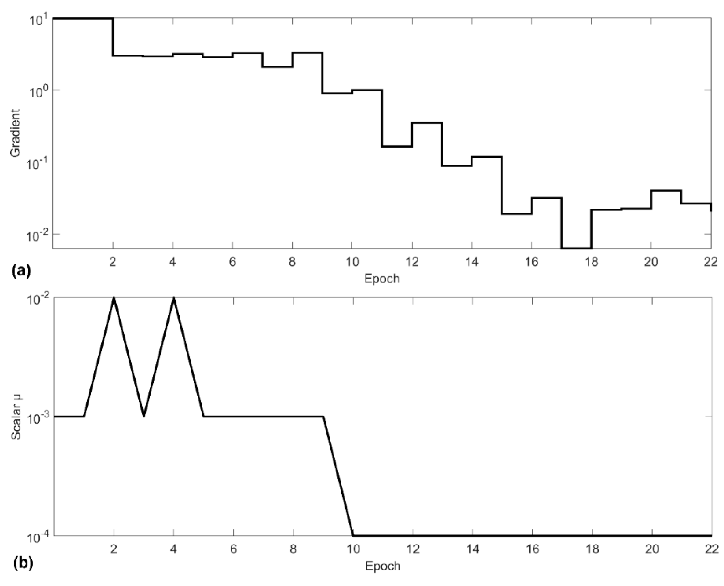
In Equation (11), is a scalar which balances the two contributions of the algorithm: Newton and gradient descent. When the scalar is zero, Equation (11) represents Newton’s method with an approximation of the Hessian matrix. With µ sufficiently large, Equation (11) represents the method of descending the gradient with a small step size. We know that Newton’s method is faster and more accurate when we are close to a minimum of error. So, our aim is to use Newton’s method as quickly as possible. Therefore, µ is decreased after each successful pass and is increased only when a temporary pass would increase the performance function [52]. Thus, the performance function is always reduced with each iteration of the algorithm. Figure 7 shows how these parameters change during the training phase.
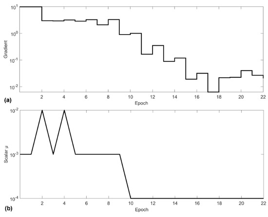
Figure 7.
Parameter changes during the training process. The term epoch refers to one cycle through the full training dataset. (a) Shows the variation of the gradient at each step performed by the algorithm for adjusting the weights of the connections, as described in Equation (7). (b) Shows how the scalar parameter µ was used to balance the two contributions of the algorithm Newton and gradient descent changes, as described in Equation (10).
To measure the performance returned by the prediction model, various metrics were adopted. A first check can be performed using a measure of the variability present between the real data and those returned by the model. Variability is the amount of dispersion present in the data. Two data sets can differ in both location and variability; or they can be characterized by the same variability, but by a different measure of position; or again, they may have the same position measure, but differ considerably in terms of variability. One measure that considers how observations are distributed or concentrated around a central trend measure is the root mean square error. The mean squared error (MSE) of an estimator with respect to the estimated parameter is defined as follows [53]:
Here,
- is the real value.
- is the predicted value.
- N is the number of the observation.
Another way to measure model performance is to use the correlation coefficient. Correlation is an index that measures the association between two variables, more specifically, it measures the degree to which two variables move together [54]. Regardless of the type of correlation index you intend to use, all indices have some common characteristics. The two sets of scores are associated with the same individuals or events, or with different subjects but associated with each other from a specific point of view. The value of the correlation index vary between −1 and +1; both extreme values represent perfect relationships between the variables, while 0 represents the absence of relationship. This at least if we consider linear relationships. A positive relationship means that individuals who get high values in one variable tend to get high values on the second variable. And vice versa is also true, that is, those who have low values on one variable tend to have low values on the second variable. A negative relationship indicates that low scores on one variable correspond to high scores on the other variable [55]. In Table 6 are shown the MSE and the correlation coefficient returned by the model.

Table 6.
MSE and R for the regression model.
The values in Table 6 tell us that the errors made in the prediction of the reverberation time are very low; specifically, there is a slight increase in the error passing from the training set to the test set. Consistent with this result, the correlation coefficient presents values very close to unity indicating a strong correlation between the real values and those predicted by the model. Additionally, in this case there is a slight decrease in R passing from the training set to the test set. These results tell us that the procedure proposed in this work can return the values of the reverberation time of a room using simple sound recordings.
4. Conclusions
Measurement of reverberation time is not an easy procedure to perform and requires the use of a space exclusively. It is in fact necessary to use instruments that reproduce a sound source and instruments to record the impulse response. In this work, an automatic procedure for estimating reverberation time based on the use of artificial neural networks was developed. At first some sounds were selected to be reproduced in the rooms, having the foresight to choose sounds that covered all the frequency ranges, with diversified characteristics. These sounds were reproduced, and joint recordings were made. The reverberation times of the rooms under observation were then measured using the integrated impulse response method. Toy balloons inflated with air were used as the sound source to produce the impulsive sound.
The recorded sounds were processed with the feature’s extraction, then they were labeled by associating to each sound the value of the reverberation time in octave bands of that specific room. The feature used was the magnitude-squared coherence estimation for the signals recorded in twelve rooms. The obtained dataset was used as input for the training of an algorithm based on artificial neural networks. Subsequently, previously unused observations were used for model validation and testing. The model returned excellent performance (R = 0.979), suggesting the use of the procedure for estimating the reverberation time of the rooms.
The evaluation of the reverberation time with the methodology described in this work is easy to carry out both in terms of instruments and in terms of people to use. On the other hand, it requires careful selection of where to place the sound source and where to place the recorder.
Author Contributions
Conceptualization, G.C. and G.I.; methodology, G.C.; investigation, G.C.; measurements, G.C. and G.I.; software, G.C.; post-processing data, G.C. and G.I.; data curation, G.C. and G.I.; writing—original draft preparation, G.C. and G.I.; writing—review and editing, G.C. and G.I.; visualization, G.C.; supervision, G.C. and G.I.; references study, G.C. and G.I. All authors have read and agreed to the published version of the manuscript.
Funding
This research received no external funding.
Institutional Review Board Statement
Not applicable.
Informed Consent Statement
Not applicable.
Data Availability Statement
Data available on request due to restrictions eg privacy or ethical.
Conflicts of Interest
The authors declare no conflict of interest.
References
- Kuttruff, H.; Schultz, T.J. Room Acoustics. Phys. Today 1974, 27, 51–52. [Google Scholar] [CrossRef]
- Cremer, L.; Müller, H.A.; Northwood, T.D. Principles and Applications of Room Acoustics. Phys. Today 1984, 37, 86–87. [Google Scholar] [CrossRef]
- Bradley, J. Review of objective room acoustics measures and future needs. Appl. Acoust. 2011, 72, 713–720. [Google Scholar] [CrossRef]
- Llorca, J.; Redondo, E.; Vorländer, M. Learning room acoustics by design: A project-based experience. Int. J. Eng. Educat. 2019, 35, 417–423. [Google Scholar]
- Vorländer, M. Computer simulations in room acoustics: Concepts and uncertainties. J. Acoust. Soc. Am. 2013, 133, 1203–1213. [Google Scholar] [CrossRef]
- Barron, M. Auditorium Acoustics and Architectural Design, 2nd ed.; Spon Press: London, UK, 2010. [Google Scholar]
- Iannace, G.; Ciaburro, G.; Trematerra, A. The acoustics of the holy family church in Salerno. Can. Acoust. 2020, 48. Available online: https://jcaa.caa-aca.ca/index.php/jcaa/article/view/3374 (accessed on 12 February 2021).
- Lundeby, A.; Vigran, T.E.; Bietz, H.; Vorländer, M. Uncertainties of measurements in room acoustics. Acta Acust. United Acust. 1995, 81, 344–355. [Google Scholar]
- Iannace, G.; Berardi, U.; De Rossi, F.; Mazza, S.; Trematerra, A.; Ciaburro, G. Acoustic Enhancement of a Modern Church. Build. 2019, 9, 83. [Google Scholar] [CrossRef]
- Sumarac-Pavlovic, D.; Mijic, M.; Kurtovic, H. A simple impulse sound source for measurements in room acoustics. Appl. Acoust. 2008, 69, 378–383. [Google Scholar] [CrossRef]
- Eaton, J.; Gaubitch, N.D.; Moore, A.H.; Naylor, P.A. Estimation of Room Acoustic Parameters: The ACE Challenge. IEEE/ACM Trans. Audio Speech Lang. Process. 2016, 24, 1681–1693. [Google Scholar] [CrossRef]
- Sabine, W.C. Architectural Acoustics. Proc. Am. Acad. Arts Sci. 1906, 42, 51. [Google Scholar] [CrossRef]
- Everest, F.A.; Pohlmann, K.C. Master Handbook of Acoustics; Copyright© 2021; McGraw-Hill Companies: New York, NY, USA, 2001. [Google Scholar]
- Puyana-Romero, V.; Núñez-Solano, D.; Molina, R.H.; Fernández-Zacarías, F.; Beira-Jiménez, J.L.; Garzón, C.; Jara-Muñoz, E. Reverberation time measurements of a neonatal incubator. Appl. Acoust. 2020, 167, 107374. [Google Scholar] [CrossRef]
- Funkhouser, T.; Tsingos, N.; Carlbom, I.; Elko, G.; Sondhi, M.; West, J. Modeling sound reflection and dif-fraction in architectural environments with beam tracing. In Proceedings of the Forum Acusticum, Sevilla, Spain, 16–20 September 2002; p. 8. [Google Scholar]
- Zotter, F.; Sontacchi, A.; Holdrich, R. Modeling a spherical loudspeaker system as multipole source. Fortschr. Akustik 2007, 33, 221. [Google Scholar]
- Yokota, T.; Sakamoto, S.; Tachibana, H. Visualization of sound propagation and scattering in rooms. Acoust. Sci. Technol. 2002, 23, 40–46. [Google Scholar] [CrossRef]
- Sabine, W.C. Collected Papers on Acoustics; Harvard University Press: Cambridge, UK, 1923. [Google Scholar]
- ISO 10534-2:1998. In Acoustics—Determination of Sound Absorption Coefficient and Impedance in Impedance Tubes—Part 2: Transfer-Function Method; International Organization for Standardization: Geneva, Switzerland, 2012.
- ISO 354:2003. In Acoustics—Measurement of Sound Absorption in a Reverberation Room; International Organization for Standardi-zation: Geneva, Switzerland, 2012.
- Abdullah, R.; Ismail, S.I.; Dzulkefli, N.N. Potential acoustic treatment analysis using sabine formula in unoccu-pied classroom. J. Phys. Conf. Ser. 2020, 1529, 022031. [Google Scholar] [CrossRef]
- Núñez-Solano, D.; Puyana-Romero, V.; Ordóñez-Andrade, C.; Bravo-Moncayo, L.; Garzón-Pico, C. Impulse re-sponse simulation of a small room and in situ measurements validation. In Audio Engineering Society Convention 147; Audio Engineering Society: New York, NY, USA, 2019. [Google Scholar]
- ISO 3382-2: 2012. In Acoustics—Measurement of Room Acoustic Param—Part 2: Reverberation Time in Ordinary Rooms; Interna-tional Organization for Standardization: Geneva, Switzerland, 2012.
- ISO 18233:2006. In Acoustics—Application of New Measurement Methods in Building and Room Acoustics; International Organiza-tion for Standardization: Geneva, Switzerland, 2012.
- Beranek, L.L. Audience and Seat Absorption in Large Halls. J. Acoust. Soc. Am. 1960, 32, 661–670. [Google Scholar] [CrossRef]
- Beranek, L.L. Concert Halls and Opera Houses: Music, Acoustics, and Architecture (Second Edition). J. Acoust. Soc. Am. 2005, 117, 987–988. [Google Scholar] [CrossRef]
- Ciaburro, G.; Berardi, U.; Iannace, G.; Trematerra, A.; Puyana-Romero, V. The acoustics of ancient catacombs in South-ern Italy. Building Acoust. 2020. [Google Scholar] [CrossRef]
- Van Gerven, M.; Bohte, S. Editorial: Artificial Neural Networks as Models of Neural Information Processing. Front. Comput. Neurosci. 2017, 11, 114. [Google Scholar] [CrossRef]
- Zador, A.M. A critique of pure learning and what artificial neural networks can learn from animal brains. Nat. Commun. 2019, 10, 1–7. [Google Scholar] [CrossRef]
- Glowacz, A. Acoustic fault analysis of three commutator motors. Mech. Syst. Signal Process. 2019, 133, 106226. [Google Scholar] [CrossRef]
- Wiener, N. Generalized harmonic analysis. Acta Math. 1930, 55, 117–258. [Google Scholar] [CrossRef]
- Champeney, D.C. Power spectra and Wiener’s theorems. In A Handbook of Fourier Theorems; Cambridge University Press: Cambridge, UK, 1987; p. 102. [Google Scholar]
- Khintchine, A. Korrelationstheorie der stationären stochastischen Prozesse. Math. Ann. 1934, 109, 604–615. [Google Scholar] [CrossRef]
- Blackman, R.B.; Tukey, J.W. The Measurement of Power Spectra from the Point of View of Communications Engineering—Part II. Bell Syst. Tech. J. 1958, 37, 485–569. [Google Scholar] [CrossRef]
- Bartlett, M.S. Periodogram analysis and continuous spectra. Biometrika 1950, 37, 1–16. [Google Scholar] [CrossRef]
- Welch, P. The use of fast Fourier transform for the estimation of power spectra: A method based on time averaging over short, modified periodograms. IEEE Trans. Audio Electroacoust. 1967, 15, 70–73. [Google Scholar] [CrossRef]
- Villwock, S.; Pacas, M. Application of the Welch-Method for the Identification of Two- and Three-Mass-Systems. IEEE Trans. Ind. Electron. 2008, 55, 457–466. [Google Scholar] [CrossRef]
- Jacobsen, F.; Roisin, T. The coherence of reverberant sound fields. J. Acoust. Soc. Am. 2000, 108, 204–210. [Google Scholar] [CrossRef]
- Chien, C.; Soroka, W. Spatial cross-correlation of acoustic pressures in steady and decaying reverberant sound fields. J. Sound Vib. 1976, 48, 235–242. [Google Scholar] [CrossRef]
- Crocker, M.J. Handbook of Acoustics; John Wiley & Sons: Hoboken, NJ, USA, 1998. [Google Scholar]
- Tronchin, L.; Bevilacqua, A. Evaluation of Acoustic Similarities in Two Italian Churches Honored to S. Dominic. Appl. Sci. 2020, 10, 7043. [Google Scholar] [CrossRef]
- Ciaburro, G.; Iannace, G.; Passaro, J.; Bifulco, A.; Marano, D.; Guida, M.; Marulo, F.; Branda, F. Artificial neural network-based models for predicting the sound absorption coefficient of electrospun poly(vinyl pyrrolidone)/silica composite. Appl. Acoust. 2020, 169, 107472. [Google Scholar] [CrossRef]
- Ciaburro, G.; Iannace, G.; Ali, M.; Alabdulkarem, A.; Nuhait, A. An artificial neural network approach to modelling absorbent asphalts acoustic properties. J. King Saud Univ. Eng. Sci. 2020. [Google Scholar] [CrossRef]
- Marquardt, D.W. An Algorithm for Least-Squares Estimation of Nonlinear Parameters. J. Soc. Ind. Appl. Math. 1963, 11, 431–441. [Google Scholar] [CrossRef]
- Hagan, M.; Menhaj, M. Training feedforward networks with the Marquardt algorithm. IEEE Trans. Neural Networks 1994, 5, 989–993. [Google Scholar] [CrossRef]
- Du, S.; Lee, J.; Li, H.; Wang, L.; Zhai, X. Gradient descent finds global minima of deep neural networks. In Proceedings of the International Conference on Machine Learning, Hualien, Taiwan, 19–22 May 2019; pp. 1675–1685, PMLR. [Google Scholar]
- Cai, T.; Gao, R.; Hou, J.; Chen, S.; Wang, D.; He, D.; Wang, L. Gram-Gauss-Newton Method: Learning Overparameterized Neural Networks for Regression Problems. arXiv 2019, arXiv:1905.11675. [Google Scholar]
- Yu, X.; Efe, M.; Kaynak, O. A general backpropagation algorithm for feedforward neural networks learning. IEEE Trans. Neural Netw. 2002, 13, 251–254. [Google Scholar] [CrossRef] [PubMed]
- Setti, S.; Wanto, A. Analysis of Backpropagation Algorithm in Predicting the Most Number of Internet Users in the World. J. Online Inform. 2019, 3, 110–115. [Google Scholar] [CrossRef]
- Lourakis, M.I. A brief description of the Levenberg-Marquardt algorithm implemented by levmar. Found. Res. Technol. 2005, 4, 1–6. [Google Scholar]
- Yu, H.; Wilamowski, B.M. Levenberg-marquardt training. Ind. Electron. Handb. 2011, 5, 1. [Google Scholar]
- Moré, J. The Levenberg-Marquardt algorithm: Implementation and theory. In Lecture Notes in Mathematicsl; Springer: Berlin/Heidelberg, Germany, 1978; Volume 630. [Google Scholar]
- Prasad, N.N.; Rao, J.N. The estimation of the mean squared error of small-area estimators. J. Am. Stat. Assoc. 1990, 85, 163–171. [Google Scholar] [CrossRef]
- Taylor, R. Interpretation of the Correlation Coefficient: A Basic Review. J. Diagn. Med Sonogr. 1990, 6, 35–39. [Google Scholar] [CrossRef]
- Benesty, J.; Chen, J.; Huang, Y.; Cohen, I. Pearson Correlation Coefficient. In Lecture Notes in Computer Science; Springer International Publishing: New York, NY, USA, 2009; pp. 1–4. [Google Scholar]
Publisher’s Note: MDPI stays neutral with regard to jurisdictional claims in published maps and institutional affiliations. |
© 2021 by the authors. Licensee MDPI, Basel, Switzerland. This article is an open access article distributed under the terms and conditions of the Creative Commons Attribution (CC BY) license (http://creativecommons.org/licenses/by/4.0/).

