Simulation of Scalability in Cloud-Based IoT Reactive Systems Leveraged on a WSAN Simulator and Cloud Computing Technologies ^†

Abstract

Implementing a wireless sensor and actuator network (WSAN) in Internet of Things (IoT) applications is a complex task. The need to establish the number of nodes, sensors, and actuators, and their location and characteristics, requires a tool that allows the preliminary determination of this information. Additionally, in IoT scenarios where a large number of sensors and actuators are present, such as in a smart city, it is necessary to analyze the scalability of these systems. Modeling and simulation can help to conduct an early study and reduce development and deployment times in environments such as a smart city. The design-time verification of the system through a network simulation tool is useful for the most complex and expensive part of the system formed by a WSAN. However, the use of real components for other parts of the IoT system is feasible by using cloud computing infrastructure. Although there are cloud computing simulators, the cloud layer is poorly developed for the requirements of IoT applications. Technologies around cloud computing can be used for the rapid deployment of some parts of the IoT application and software services using containers. With this framework, it is possible to accelerate the development of the real system, facilitate the rapid deployment of a prototype, and provide more realistic simulations. This article proposes an approach for the modeling and simulation of IoT systems and services in a smart city leveraged in a WSAN simulator and technologies of cloud computing. Our approach was verified through experiments with two use cases. (1) A model of sensor and actuator networks as an integral part of an IoT application to monitor and control parks in a city. Through this use case, we analyze the scalability of a system whose sensors constantly emit data. (2) A model for cloud-based IoT reactive parking lot systems for a city. Through our approach, we have created an IoT parking system simulation model. The model contains an M/M/c/N queuing system to simulate service requests from users. In this use case, the model replication through hierarchical modeling and scalability of a distributed parking reservation service were evaluated. This last use case showed how the simulation model could provide information to size the system through probability distribution variables related to the queuing system. The experimental results show that the use of simulation techniques for this type of application makes it possible to analyze scalability in a more realistic way.

1. Introduction

The paradigm of pervasive systems permits to connect devices that may have some intelligence capacity. These devices can send information about data of the physical world in real time: temperature, state of illumination, levels of CO₂, etc. In the health sector, pervasive systems can monitor patients’ vital signs in real time, or pervasive systems can establish control of important assets in a certain hospital, where they are and how they are used, and so on. In smart cities, the use of these technologies helps the control of pollution, street lighting, traffic management, etc. [1].

The possibility of implementing Internet of Things (IoT) applications with the deployment of large numbers wireless sensor and actuator networks (WSANs), where it could include scenarios with mobility, motivates preliminary analyses in which simulation can play a relevant role. The simulation of systems with heterogeneous and large-scale scenarios is a complex task. The evaluation of the parameters that involve this type of system needs tools that support the interaction between different scenarios.

Ptolemy II is an open-source software framework supporting experimentation with actor-oriented design [2]. A model is a hierarchical interconnection of actors, which execute concurrently and communicate through messages sent via interconnected ports. Each level of the hierarchy in a model can have its own director, and distinct directors can be composed hierarchically. System modeling through the design hierarchy provided by Ptolemy II helps extend the model to simulate the growth and expansion of WSANs over large areas such as a set of city parks.

Internet of Things (IoT) enables the connection of identifiable physical world objects with cyberspace through Internet communications. IoT uses radiofrequency identification (RFID), quick response (QR) codes, sensor, or wireless technology to enable intercommunication between devices. Additionally, the IoT ecosystem can consist of a set of components such as smart objects, intelligent devices, smartphones, and tablets [3]. In general, the IoT paradigm can help to design innovative services that involve the use of WSANs or smartphones as sensor technologies. These technologies can use the MQTT (message queue telemetry transport) protocol for the transfer of sensed data because it consumes very little bandwidth.

The systems development process for IoT applications in a smart city requires preliminary research on the components and the interaction between them to achieve the proofs of concept and obtain verified prototypes [4]. This process involves a series of components such as IoT sensors, communications elements, software services, and data repositories. Thus, building prototypes of an IoT system with some real sensor nodes for a smart city that meets certain needs could be impractical during experimental tests.

Modeling and simulation are alternative techniques that facilitate the analysis, design, and experimental testing of IoT applications. We find these techniques relevant to the construction of the sensor network model. Some advantages of using the simulation are the acceleration of the tests, the saving of costs, the minimization of risks, and the preliminary analysis of characteristics such as the performance of the system. In this way, it is possible to do a scalability analysis, define the variables handled, or know the types of sensors. Despite these advances, simulators for IoT applications that consider the functionality of end-to-end services are an open line of research [4]. Although we have followed some simulation methods and principles described in the literature [5,6], the complete validation of the simulation models is beyond the scope of this paper. However, we performed several simulation experiments to verify the models and achieve the research objectives.

In recent years, different technologies around modern cloud computing infrastructures have evolved allowing one to streamline development and operations tasks (Google Cloud Platform, Kubernetes (K8s), and Docker containers). These technologies allow a flexible development and integration process of the system components and facilitate monitoring and scalability [7]. Additionally, IoT software services can be modeled using microservices design patterns. Thus, it is possible to have simulation tests in a more realistic way using a cloud computing infrastructure and leaving aside the cloud computing simulation tools. Additionally, some of the concerns related to distributed application modeling can be addressed through the use of the principles of reactive manifesto. These principles can be applied to achieve reactive applications that use observable models, event streams, and stateful clients [8].

This article proposes an approach for the modeling and simulation of IoT systems and services in smart cities leveraged on a simulator of WSANs and technologies of cloud computing. The main objective is to facilitate the modeling of IoT systems for the design and experimental verification before the actual construction of this type of system. Focused on the use of microservices, we provide an approach that helps to model and simulate IoT reactive web services (using Finite State Machine (FSM) and other patterns) with the elements for real-time data collection, transfer, and storage based on the idea of using reactive components. Our approach was verified through experiments with two use cases.

The first use case was the construction of a WSAN model of an IoT system for the monitoring and control of a city park. This WSAN was used to simulate the data collection of certain physical variables. This model was extended by replication using Ptolemy’s hierarchical modeling capacity to model an IoT application for the control and monitoring of multiple parks in a city. Through this use case, we analyze the hierarchical modeling and scalability of the system whose sensors constantly emit data. This first verification of our approach was carried out with all the components of the system model locally [9]. Thus, we show the basic use of our approach when modeling a simple IoT application that does not require interactions with microservices in the cloud platform.

The second use case is related to the scenario of the parking reservation service of a city. We build a model of a cloud-based IoT reactive parking lot system. Additionally, the service request of the system users was simulated using an M/M/c/N queuing system. The data simulations were based on certain values generated through probability distribution variables. Additionally, our approach has considered the design-time verification of some aspects, such as the sensor network’s dimensioning, the delimitation of web services, and components’ performance.

Contribution. Our study makes the following contributions.

• Model of a wireless sensor network as part of a simple IoT application to monitor and control constantly the parks of a city.
• Model of a wireless sensor network as part of an IoT application that provides service to users with an M/M/c/N queuing system.
• Model of infrastructure for the support of reactive web services in the cloud platform to simulate IoT applications.

We show the potential use of our approach for the replication of simulation models (parameterizable and modifiable) for the scalability of simulation models. Additionally, the models help us evaluate the resizing and performance of IoT systems. The characteristics of our approach are valuable in the preliminary design and the construction of prototypes of applications of IoT in a smart city.

Organization. The remainder of this article is organized as follows. Section 2 discusses related works. Our modeling and simulation architecture to support the proposed approach is described in Section 3. The implementation of the use case on the IoT system for park monitoring and control is presented in Section 4. We detail the composition process to create a parking lot system model in Section 5. The results are presented and discussed in Section 6 through the use of our approach in simulating the scenarios of the analyzed use cases. Finally, Section 7 presents conclusions and future work.

Extended part. Based on our previously published work [9], our article includes new components to the architecture for the modeling, simulation, and study of the scalability of more complex IoT systems. Major extended parts are as follows. In Section 2, the related works was updated to compare our approach with other alternatives for simulating IoT systems. In Section 3, we expanded the modeling and simulation architecture to take advantage of the facilities offered by the cloud providers to rapidly deploy new components for the system architecture using containers. Additionally, an alternative for flexible microservices modeling was introduced through the use of Akka FSM. In Section 5, a new and more complex use case was introduced through the construction of the IoT parking lot system model that includes microservices modeling. The new results obtained from the study of the scalability of the IoT reactive parking lot system model were shown and discussed in Section 6

2. Related Works

An interesting survey [4] categorizes IoT simulators into three groups. In the first group, we had simulators with support for end-to-end simulations of IoT applications, the next category includes those simulators with IoT applications with big data treatment, and finally the last category groups the general network simulators.

In the first category, we could find DPWSim and iFogSim. DPWSim simulated IoT applications using web services on smart and resource-constrained devices, which was supported by the Organization for the Advancement of Structured Information Standards (OASIS). DPWSim is not compatible with other existing protocols [10]. iFogSim models and simulates fog and edge computing environments, but procedures for modeling IoT nodes are not addressed [11].

Among the big data processing simulators, we had IOTSim and SimIoT. IOTSim [12] uses the MapReduce model for big data processing of IoT applications but does not handle interactions with the sensor network or the stream processing paradigm. SimIoT [13] helps evaluate job processing times in a cloud-based system, but it does not have distributed processing capabilities, and sensor communication simulation techniques are essential.

There are many tools available such as general-purpose network simulators that can be commercial and open-source, such as OMNeT ++ [14], ns-3 [15], NetSim [16], and QualNet [17]. They help to simulate the behavior of wired networks or wireless networks by visualizing data flows, analyzing network performance, and obtaining the cost of network design [18]. However, support for IoT application-level standards protocols is not available. Additionally, commercial simulators have a very expensive license with limited use on certain platforms. For example, the NetSim version can only be used on Windows platforms and its price is quite high.

Table 1. Summary of tools to support Internet of Things (IoT) simulation. Y: Supported, N: Not Supported.

Simulator	Ref.	Category	Language	Modelling IoT Nodes	Cloud Layer	Application Layer
DPWSim	[10]	Full Stack Simulator	Java	N	N	Y
iFogSim	[11]	Full Stack Simulator	Java	N	Y	Y
IOTSim	[12]	Big Data Processing	Java	N	Y	Y
SimIoT	[13]	Big Data Processing	Java	N	Y	Y
OMNeT++	[14]	Network Simulator	C++, Java, C#	Y	N	N
ns-3	[15]	Network Simulator	C++, Python	Y	N	N
NetSim	[16]	Network Simulator	Java	Y	N	N
QualNet	[17]	Network Simulator	C/C++	Y	N	N
Our hybrid solution	[This]	An approach to Full Stack simulator	Java, JavaScipt, Scala & HTML5	Y	Y	Y

provides a comparison between the IoT simulators discussed above and our proposed approach.

3. The Modeling and Simulation Architecture

3.1. Work Environments

The simulation environment is divided into two parts. The first part contains all the elements used to simulate a WSAN, and the second part is made up of the components to be deployed in the cloud platform. Some of the concerns related to distributed application modeling can be addressed by using elements that follow the principles of reactive manifesto. These principles help to design reactive applications that use observable models, event streams, and stateful clients [8]. Figure 1 shows the architectural components and their interrelationships. This architecture has real-time features that are essential to meet some needs of IoT applications. The set of components deployed in the cloud platform can be used as a common architecture for data transfer of multiple applications and services in a smart city.

Through our approach, it is feasible to run several simulation files of the model of an IoT system. The simulation can scale through simulation files with a hierarchical structure of several IoT models on the same computer. Additionally, it is possible to scale the simulation further with other computers where the simulation XML files can be run.

3.2. Ptolemy II Modeling Tool: Building WSAN Models

We used Visual Sense for modeling and simulating the WSAN. Visual Sense is a framework for building models that include sophisticated elements from various aspects and is built on Ptolemy II. Visual Sense provides facilities for modeling communication channels, sensor channels, ad-hoc network protocols, media access control protocols, power consumption at sensor nodes, etc. [19,20].

A characteristic to highlight in the elaboration of a WSAN model is the use of “Accessors” of Ptolemy II [21]. Accessors extend the applicability of Ptolemy to modeling IoT systems, allowing models to communicate with the computer’s input and output interfaces. Our model uses the accessors for communication with an MQTT Message Broker: accessor-net/MQTT-Publisher and accessor-net/MQTT-Subscriber.

3.3. Component Infrastructure in the Cloud Platform

Some of the benefits of using the cloud platform are flexible system capacity, scalability adjustment, and elasticity. Cloud providers such as Amazon Web Services and Google Cloud Platform offer the use of virtual machines where we can deploy the components of the architecture. They also provide Kubernetes as a portable, extensible, open-source platform for managing containerized workloads and services [22]. Thus, we use images of containerized system components by using Docker technology to deploy our architecture [23].

The main component that makes possible the union of the WSAN simulation environment and the cloud components is an MQTT Broker. The MQTT protocol is useful due to its low bandwidth requirement, is easy to implement, and can be used for some types of environments where devices with limited resources are used, such as in a WSAN [24]. In this paper, we used the Erlang MQTT Broker (EMQ/eMQTT). eMQTT is a distributed, massively scalable, highly extensible MQTT message broker written in Erlang/OTP [25]. In Docker Hub, there are many images about an eMQTT [26].

Furthermore, we used Apache Kafka to facilitate the construction of fast data ingestion architectures, making it possible to build near-real-time web applications through the management of streaming data pipelines [27].

Moreover, we used MongoDB as a system data repository. MongoDB is a distributed, document-based database that offers more flexibility and high performance than relational databases [28].

Finally, IoT software services are containerized and deployed as microservices. The microservices are designed using an asynchronous, nonblocking, message-driven approach to improve the user experience [29].

3.4. Microservices Modeling with Akka FSM

Microservices architecture can be used as a distributed computing architecture to build system software components [30]. These software components are business logic for applications that interact with the end-user or flexible components for machine-to-machine communication using a message broker.

Distributed applications can be made up of stateless and stateful components. Stateless microservices have some advantages over stateful microservices. For example, the failure of an individual instance does not have a significant impact on the system because the new instance can replace the current instance. Another example is the deployment of a new version of stateless microservice that is easier since the microservice with the old version can just be stopped and replaced without having to migrate its state [30]. However, there may be functionalities in systems that need to preserve the system state during their operation, which requires the design of stateful components.

Akka FSM technology is based on the Akka actor model. The actor model provides a higher level of abstraction for writing concurrent and distributed systems. It helps the programmer from having to deal with explicit locking and thread management, making it very easy to write correct concurrent and parallel systems [31].

3.5. Security

In our approach, we considered minimal characteristics related to the security of the data processed in the simulation processes, to provide similarity to a real environment. Some protocols and technologies were selected to maintain the security of data transfer and storage.

The EMQ broker guarantees the authentication of MQTT clients with client ID, username/password, IP address, and even HTTP cookies [32]. Confluent provides transport layer security (TLS) encryption, simple authentication and security layer (SASL) authentication, and authorization via access control lists (ACLs) [33].

Regarding data storage, MongoDB facilitates authentication through the salted challenge response authentication mechanism (SCRAM) and x.509 certificate authentication. Additionally, MongoDB employs role-based access control (RBAC) to govern access to a MongoDB system and supports transport layer security and secure sockets layer to encrypt all of MongoDB’s network traffic [34].

On the other hand, some of the components of our system are supported on the Google cloud infrastructure whose security is designed in layers that include physical components and data centers, secure communication between services, protected access to services from the Internet, etc. [35] Additionally, K8s also provides some possibilities to configure node, container, and pod security [36].

4. Modeling an IoT System to Monitor and Control the Parks of a City

In this article, the authors modeled an application of IoT to monitor and control the parks of a city. A system was designed that monitors and controls a total of 10 parks each of which has homogeneous characteristics. Each park (that is basically a WSAN) was modeled with a total of 10 sensors, which transmit the data related to solar radiation, carbon dioxide, ambient temperature, and air humidity. In addition, one more sensor provides the status of the water sprinklers and an actuator for opening or closing the sprinklers. Figure 2 illustrates each of the sensors and the actuator, which are located at a certain distance from the Gateway. In this way, the Gateway receives the signals without a loss of data (the power propagation factor is 1.0/(4 × PI × distance × distance)) [20]. For simplicity, Figure 3 summarizes the distribution of the sensors and the actuator. Figure 4 illustrates the model of a park in a city as a black box.

Certain data generators were constructed that simulate the data of the physical variables to be monitored. Data generators produce a random sequence with Gaussian distribution. The mean of the random numbers for each physical variable were: solar radiation = 100 W/m², carbon dioxide = 200 mg/m³ (1 ppm = mg/m³), ambient temperature = 20 °C, and air humidity = 40% RH.

The network was built with the sensors, which were modeled as generators data samplers of the physical variables. These sensors collect the data in a given node, which sends the data to the central node of the park. The central node is a sink node and transmits the data to a Gateway. From the Gateway, an accessor-net/MqttPublisher (MQTT Client) finally sends the data to the Message Broker and an accessor-net/MqttSubscriber receives data to control the sprinklers. The network was modeled using the conventional discrete-event (DE) models with the basic concepts of power propagation and power loss channel [20].

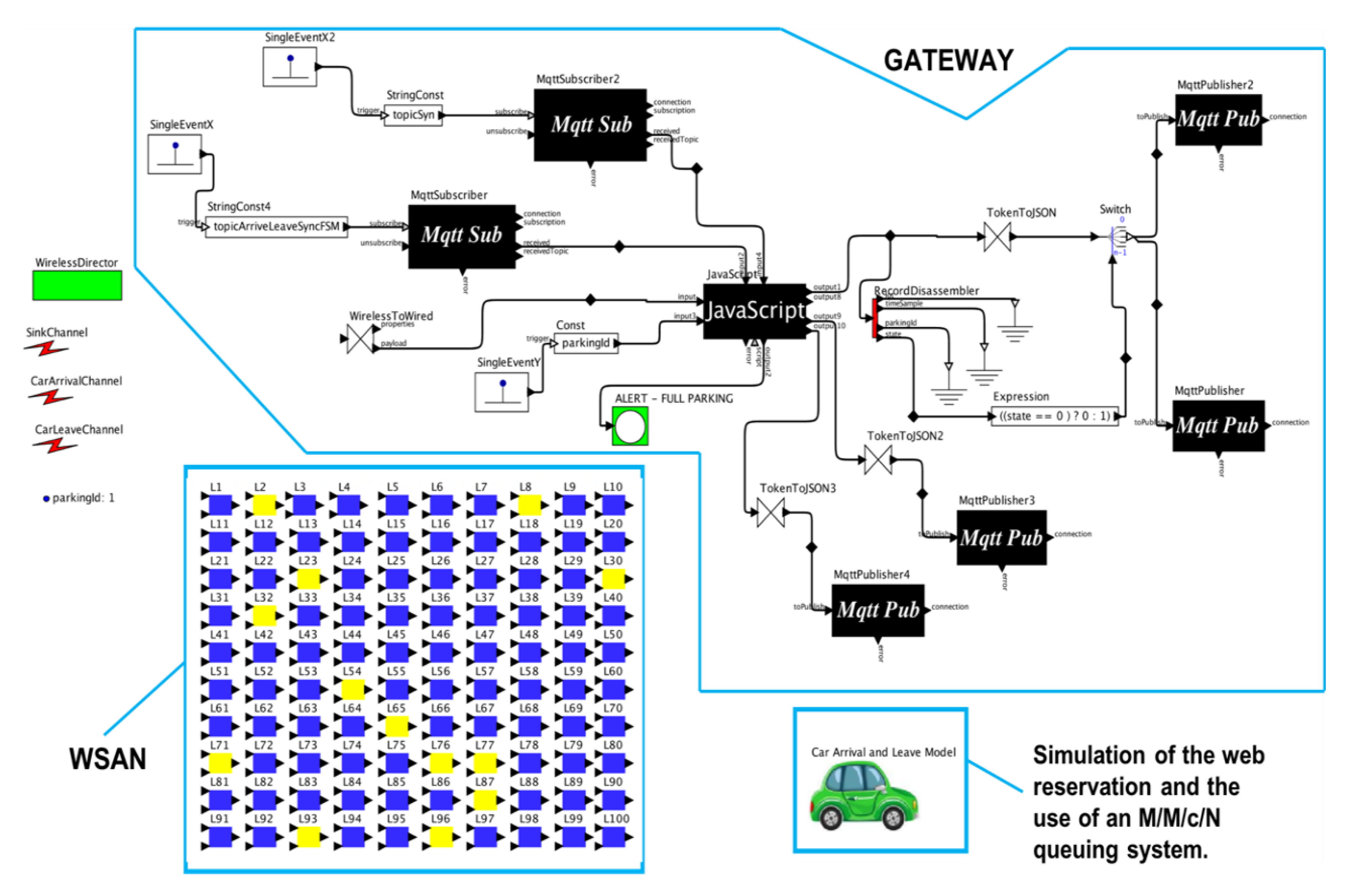
5. Building IoT Parking Lots Reactive System Model

5.1. Scope and Context

A basic scenario was established for the modeling of the system, which includes a set of concerns related to the need to use a parking lot in a city. The extended version of the basic scenario is based on the use of multiple parking lots. The scenario considers the need to use a parking space in a parking lot for a certain time. Drivers can request a reservation number that is provided by the system that controls the parking spaces. The IoT parking reservation system is comprised of a subsystem in the parking lot that consists of a WSAN. The sensors send the data to the cloud platform in real time as messages about the change of state of the parking spaces (occupied or unoccupied).

Additionally, the IoT parking reservation system has a web application hosted in the cloud platform with functionalities to manage the maintenance of the system status (number of available parking spaces) and to make the reservation of parking spaces.

The reservation request is made using a web service through a computer or a smartphone. Thus, the user accesses the web application to request the reservation by entering their user identification and the parking lot Identification. When the system has parking spaces, the system responds with a QR code containing the assigned reservation number, otherwise the system rejects the request. The WSAN actuators can receive notifications of the reservation assignment service in such a way that the parking spaces are physically reserved and cannot be used. Vehicle access to the parking lot can only be done with the assigned QR code. Monitoring service to check the status of the parking spaces is necessary to know in real time the availability of reservations.

Finally, the system must take into consideration the possible interruption of the web application, its reinitialization, and the restoration of the state of the IoT parking reservation system.

5.2. Reservation System General Model

The solution includes three well-differentiated parts (1) the set of technologies that are in the parking lot, which are basically a WSAN, (2) the communication infrastructures, and (3) the web application hosted on a web server in the cloud platform. Figure 5 illustrates the macro model of the system. The WSAN contains a set of actuators and sensors that help keep the states of the parking spaces up to date. The sensors/actuators generate MQTT messages of the status changes of the parking spaces. The parking lot has a Gateway through which messages from other parts of the system are sent or received. Other situations in which the states of the parking spaces are transmitted to the web application are: (1) the start of some monitoring process from the web application or (2) when there is a failure of the web application that involves the reinitialization of the system.

The communication channel between the WSAN and the Web application was built through a channel formed by an MQTT broker Cluster [25], an MQTT-Kafka Bridge, and a Confluent Kafka broker cluster [37].

The web application is hosted in the cloud platform and contains all the web services designed to meet the requirements of the IoT parking reservation system. The modeled services were:

• Stateless basic services for the management of system data such as user data and parking lot data.
• A stateful service for the maintenance of the state of the system (number of parking spaces available) and reservation allocation. This service contains the operational components for synchronization with the WSAN and the recovery of the state of the parking spaces. These operational components are useful during startup or restart of the web application due to possible service interruptions.
• A stateless service for reservation request that provides the user with the QR code of the reservation.
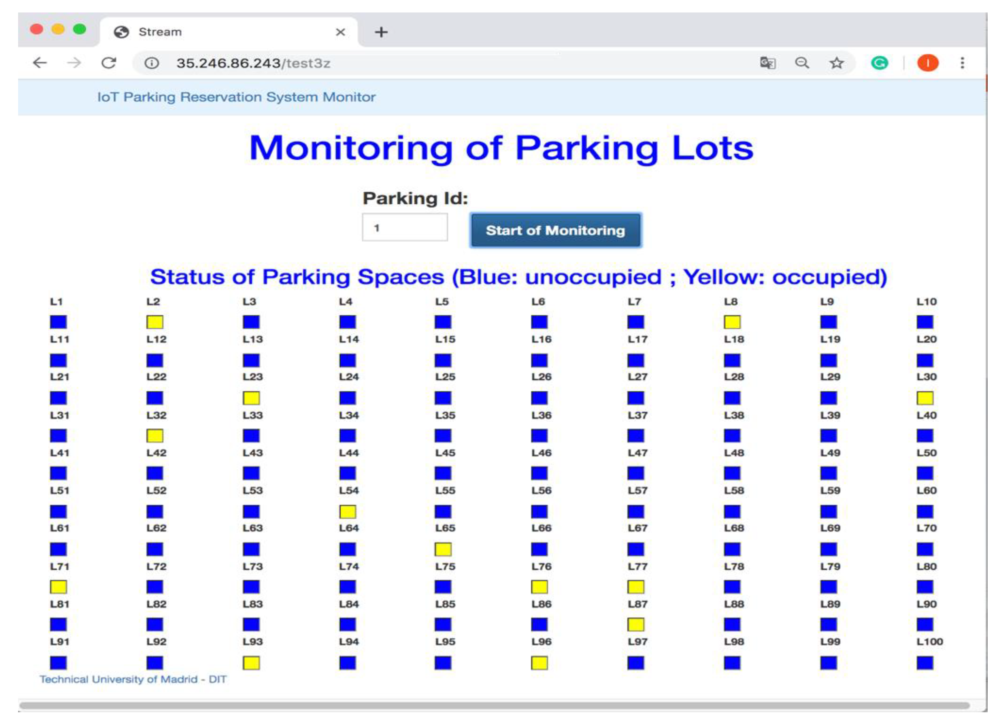
• A stateless service to monitor the status of parking spaces in real time.

5.3. Developing an IoT Parking Lot Model Based on a WSAN

The parking lot is essentially a WSAN that was developed with VisualSense. Figure 6 shows the parking lot model with 100 parking spaces, each one consisting of a sensor and an actuator. All sensors/actuators communicate wirelessly to the Gateway that contains an MQTT Pub Client and an MQTT Sub Client (MQTT-Publisher accessors and MQTT-Subscriber accessors). The Gateway communicates with the cloud platform through an MQTT Broker.

5.4. Developing Vehicle Arrival/Departure Submodel

Due to the objectives of this research in conducting accelerated simulations of the IoT parking reservation system (without depending on the reservation through web services), a submodel was created that simulates the pattern of arrival and departure of vehicles. Furthermore, to simplify the model, it was assumed that the time difference between the allocation of the reserve and the arrival of the vehicle at the parking lot is negligible. Regardless of this, the reservation allocation service guarantees the update of the reservation in simulations with the reservation request service.

The vehicle arrival/departure submodel was designed using an M/M/c/N queuing system. The M/M/c/N queuing system used an exponential interarrival or service time distribution with a queue discipline FIFO (first-in, first-out).

Figure 7 illustrates the model of vehicle arrivals and departures. When the reservation of a parking space was simulated (the sensor changes to yellow), an MQTT message (“topicArrivals”) was generated and sent to the web application that controls the reservations. Similarly, when a vehicle leaves the parking lot (the sensor turns blue), an MQTT message (“topicDepartures”) was generated and sent to the web service that controls reservations. The information in the MQTT message was used to maintain the reserve status of the system.

Besides, the components that interact with the synchronization services were incorporated into the model to obtain the states of the parking spaces. Thus, accessors were added for the following synchronization operations:

• Synchronization by monitoring (“topicSyncManualScreen” and “topicSyncManualScreenData”), and
• Synchronization due to web server failure (“topicSyncStartFSM” and “topicSyncStartFSMData”)

5.5. Developing the Microservices Model for the IoT Parking Lot System

Table 2. Microservices and used patterns.

Microservices	Patterns
User Data Service	MVC
Parking Lot Data Service	MVC
Reservation Request Service	MVC
Monitoring Service	MVC Messaging (Publish/Subscribe)
Reservation Allocation Service	Akka FSM Actor Messaging (Publish/Subscribe)

shows the patterns used to model system services.

• The MVC pattern is the model–view–controller design pattern that helps implement microservices made up of visual interfaces.
• The message pattern is useful for implementing services that contain communication functionalities with message brokers.
• The Akka FSM actor pattern was used to implement services whose functionality could be expressed as a set of interrelated states in concurrency.

The implementations were carried out mainly through the play framework and the Scala programming language.

5.5.1. Stateless Services

Basic Services and the Reservation Request Service

Figure 8 shows the main interface from which the system functionalities were selected. The user data and parking lot data options facilitate the management of user data and data of the parking lots registered in the system. Besides, the Reservation Request Manager option gives access to the reservation request operation, as shown in Figure 9.

The Monitoring Service and the Synchronization Algorithm

Figure 10 shows the interface of the monitoring service. The interface visualizes the states of the parking spaces through a dashboard. The interface shows, for example, that parking space L2 was reserved (yellow), and L7 was available (blue), which coincides with our parking lot simulator in Section 5.3. The service was implemented through an additional synchronization mechanism with the WSAN Gateway.

The Gateway keeps exact data on the current status of the parking spaces (occupied or unoccupied). The Gateway is subscribed to the topic “topicSyncManualScreen” to receive synchronization messages to which the Gateway responds by publishing data with the topic “topicSyncManualScreenData”. The data received by the monitoring service were used to show the states of the parking spaces. The synchronization process is summarized as follows (see Figure 11):

• The monitoring web service sends a synchronization request message to the confluent (Kafka)
• The Gateway receives the synchronization request message from the MQTT broker.
• The Gateway sends the synchronization data to the MQTT broker.
• The monitoring service collects the synchronization data from the confluent (Kafka).
• The service shows the states of each of the parking spaces on the dashboard.

Other alternative mechanisms to preserve the data of the states of the parking spaces are possible, such as keeping the data in the memory of the web server or recovering the data from the database. However, the implementation carried out through the programming of the communication mechanisms of the MQTT and Kafka brokers was dynamic and fast. The implemented synchronization collected the data from the source and did not depend on database reads or loss of data in memory due to system failures.

5.5.2. Service Stateful Service: Reservation Allocation Service

Figure 12 shows the interaction of the system components with the reserve allocation service. The model of this service was carried out through the design of several states, which were used to maintain control of the number of available reserves. The reservation request service got a reservation number from the reservation allocation service.

The reservation request and reservation allocation include the following situations:

1. The reservation allocation service is kept “waiting” for reservation requests.

2. If (the reservation request can be attended)

Then {The FSM goes to the state “Generate Reservation/QR Code”, at the same time a message with the reservation code is sent to the reservation request service}.

Else {A message is sent to the reservation request service indicating that the parking lot is Full}

3. At any moment, the FSM attends to the incoming messages from the WSAN. If any vehicle leaves the parking lot, at that moment, the FSM goes to a state of updating the total number of parking spaces available.

An Akka FSM actor helps design the behavior of complex systems consisting of a set of coupled states as a model of concurrent states. Figure 13 shows the reservation allocation service modeled with an Akka FSM actor. The diagram illustrates the states and concurrent behavior that may exist throughout the life of the service. This stateful service uses the number of reservations available as a state variable. The service may be in a specific state, depending on the events to be attended to.

• The service model consists of the following parts:
• The states: S1 (WaitingParkingRequest), S2 (ProcessParkingRequest), S3 (CarDepartureParking-Process Kafka Message), and S4 (Common Code). S4 was used to manage the common state code as a generic event control.
• The events: E1 (ParkingRequest), E2 (PendingRequest), E3 (CarDepartureParking), E4 (Done1), and E5 (Executed2).
• Transitions: T: 1-2, T: 1-3, T: 2-1, T: 3-1

In a more general scheme, it is possible to simulate the operation of multiple parking lots around a city and build an Akka FSM actor for each of the parking lots. The Akka FSM actors can manage the allocation of the parking space reservations available in each parking lot, as shown in Figure 14.

6. Results and Discussions

6.1. Simulation of the Monitoring and Control of the Parks of a City

Initially, we carried out a sensitivity analysis of the model parameters. Then, we performed the experiments taking into consideration the scale of the number of parks within our model and observing the execution time used by the simulator.

6.1.1. Simulation Set-Up

Figure 15 illustrates each of the 10 parks, which are located around a city. For simplicity, Figure 16 illustrates a summary of the model of the IoT application with the 10 parks.

For the implementation, the authors used:

• macOS Sierra version 10.12.3, 2 GHz Intel Core i5, 8GB of memory;
• Ptolemy II 10.0 and VisualSense;
• EMQTTD Erlang MQTT Broker 1.0;
• JRE: 1.8.0_112-release-408-b6 x86_64, JVM: Open JDK 64-Bit Server VM;
• Docker Machine 0.12.2.

6.1.2. Sensitivity of the Model Parameters of the Park Monitoring System

In this section, we carried out the sensitivity analysis to study the effect of the model parameters of the control and monitoring system of parks in a city. In the following simulation experiments, we observed the effect on system performance (number of messages sent during a given time) by varying the number of sensors per park (ns), the number of parks (p), and the sampling period of the sensors to collect the data (sp).

The Effect of the Number of Sensors

First, we observed the effect of varying the number of sensors on the number of messages collected (nmsg) during a simulation time of 300 s, given that the sampling period sp = 0.94 s was a fixed value. At the same time, various scenarios related specifically to the total number of parks were used.

Table 3. Effect of the number of sensors ns and the number of parks p on the number of messages collected during 300 s, with a sampling period sp = 0.94 s.

	nmsg
	p = 1	p = 2	p = 3	p = 4	p = 5
ns = 2	604	1208	1812	2416	3020
ns = 4	1208	2416	3624	4832	6040
ns = 6	1812	3624	5436	7248	9060
ns = 8	2416	4832	7248	9664	12,080
ns = 10	3020	6040	9060	12,080	15,100

shows that the increase in ns in the monitoring processes increased the value of nmsg. Additionally, the increase in p produced an increase in the number of messages since this is related to the introduction of new sensors.

The Effect of the Sampling Period Used by the Sensors

Finally, we observe the effect of varying the sampling period on the number of messages collected (nmsg) during a simulation time of 300 s, given that the total number of sensors per park ns = 6 was a fixed value. At the same time, various scenarios related specifically to the total number of parks were used. In

Table 4. Effect of the sampling period sp and the number of parks p on the number of messages collected during 300 s, with the total number of sensors ns = 6.

	nmsg
	p = 1	p = 2	p = 3	p = 4	p = 5
sp = 0.94	1812	3624	5436	7248	9060
sp = 1.88	936	1872	2808	3744	4680
sp = 3	594	1188	1782	2376	2970
sp = 5	366	732	1098	1464	1830
sp = 7	264	528	792	1056	1320

, we observe that nmsg decreased as the value of the sampling period increased, that is, the data was collected more slowly from the sensors. Additionally, the increase in p produced an increase in the number of messages since this was related to the introduction of new sensors.

From the analysis, we could say that the change in the value of sp had an effect that was reversed to the change in ns and p. Furthermore, ns and p similarly affected the system.

6.1.3. Experiment 1

Number of computers: 1;

Number of simulators: 1;

Number of parks per simulator: 1;

Total number of sensors per park: 11;

Sampling period per sensor: 9.4 s;

Total number of actuators per park: 1;

Number of messages sent to the Broker per sensor: n.

In this experiment, a single instance of the simulator was run on the same computer with the WSAN model of a single park. At each execution, the number of messages sent by each sensor to the Message Broker was increased by 50. The details are presented in

Table 5. Experiment 1.

Execution Number	Number of Messages per Sensor (n)	Total Number of Messages Sent to Broker	Average of Execution Time (min)
1	50	550	8.29
2	100	1100	16.70
3	150	1650	25.18
4	200	2200	33.42
5	250	2750	41.83
6	300	3300	50.18
7	350	3850	58.29
8	400	4400	66.67
9	450	4950	74.99
10	500	5500	83.29

.

For example, in execution number 4, each of the sensors sends 50 messages giving a total of 4 × (50 messages/sensor) × (11 sensors) = 2200 messages. In this case, the simulation lasted 33.42 min.

There is a directly proportional relationship between the number of messages and the time taken to send the messages to the Message Broker, as shown in Figure 17.

Slope of the line = (5500 − 550)/(83.29 − 8.47) = 66 messages/minute = 1 messages per second (approximately).

6.1.4. Experiment 2

Number of computers: 1;

Number of simulators: m;

Number of parks per simulator: 1;

Total number of sensors per park: 11;

Sampling period per sensor: 9.4 s;

Total number of actuators per park: 1;

Number of messages sent to the broker per sensor: 50.

In this case, simulator-1 took a little longer when sending its 550 messages to the Message Broker. The increase is about 1 min longer for each run in which a simulator (with the same model) was added in parallel. The details are presented in

Table 6. Experiment 2.

Execution Number	Total Number of Simulators (m)	Total Number of Messages Sent to Broker	Average of Execution Time Simulator 1 (min)
1	1	550	8.29
2	2	1100	8.65
3	3	1650	8.79
4	4	2200	9.06
5	5	2750	9.17
6	6	3300	9.66
7	7	3850	10.49
8	8	4400	10.57
9	9	4950	11.65
10	10	5500	11.94

, and Figure 18 shows the effects on simulator-1.

For example, in the execution number 8, the simulator-1 took 10.57 min to send its 550 messages. This was (550/10.57)/60 = 0.87 messages per second.

6.1.5. Experiment 3

Number of computers: 1;

Number of simulators: 1;

Number of parks per simulator: p;

Total number of sensors per park: 11;

Total number of actuators per park: 1;

Number of messages sent to the broker per sensor: 50.

In this case, several city parks were simulated, which sent data to the Message Broker. In this experiment, for each execution, the number of parks was increased by one, and the sampling period was increased by 9.4 s. The details are presented in

Table 7. Experiment 3.

Execution Number	Number of PARKS	Total Number of Sensors in p Parks	Sampling Period per Sensor (sp) (s)	Total Number of Messages Sent to Broker	Average of Execution Time (min)
1	1	11	9.4	550	8.32
2	2	22	18.8	1100	16.39
3	3	33	28.2	1650	24.42
4	4	44	37.6	2200	33.42
5	5	55	47	2750	41.07
6	6	66	56.4	3300	48.93
7	7	77	65.8	3850	57.10
8	8	88	75.2	4400	65.53
9	9	99	84.6	4950	75.18
10	10	110	94	5500	80.99

. Figure 19 shows an approximation of the linear relationship between the times used by the simulator to send a certain number of messages.

In general, the simulator sent 67.176 messages per minute (1.12 messages per second), which represents the initial frequency that has been maintained due to the effect of doubling the value of the sampling period and doubling the number of sensors in each execution. In short, the increase in the number of parks in the simulation model increased the number of messages that were sent to the Message Broker if we keep or decrease the sampling period used in the sensors. Increasing the value of the sampling period in each sensor helps to reduce the number of messages sent concurrently from the parks.

6.1.6. Experiment 4

Number of computers: 1;

Number of simulators: 2;

Number of parks per simulator: p;

Total number of sensors per park: 11;

Total number of actuators per park: 1;

Number of messages sent to the broker per sensor: 50.

This last experiment was similar to experiment 3 but with two simulators on the same computer.

The details are presented in

Table 8. Experiment 4.

Number of Parks per Simulator	Total Number of Sensors per Simulator	Sampling Period per Sensor (sp) (s)	Total Number of Messages per Simulator	Average ofExecution Time Simulator 1 (min)	Average ofExecution Time Simulator 2 (min)
1	11	9.4	550	8.27	8.25
2	22	18.8	1100	16.58	16.56
3	33	28.2	1650	24.67	24.63
4	44	37.6	2200	33.16	33.00
5	55	47	2750	41.15	41.14
6	66	56.4	3300	49.70	49.62
7	77	65.8	3850	57.80	57.64
8	88	75.2	4400	66.24	66.16
9	99	84.6	4950	74.90	74.95
10	110	94	5500	82.61	82.45

. Figure 20 shows an approximation of the linear relationship between the times used by the simulator-1 and simulator-2 to send a certain number of messages. In general, simulator-1 sent 66.351 messages per minute (1.11 messages per second) and simulator-2 sent 66.399 messages per minute (1.11 messages per second). In short, the increase of another simulator in parallel in the same computer kept the sending rate of messages approximately in the same values as in experiment 3. Using two simulators, the number of messages per minute sent to the MQTT broker can be represented as y = y1 + y2 = 132.75x + 13.3138, so using the two simulators we could send 132.75 messages per minute (2.21 messages per second).

6.1.7. Message Broker, Data Monitor, and Files.xml

The messages were sent from the simulators to the Message Broker. The Data Monitor collects the messages from the Message Broker (see Figure 21 and Figure 22).

The experiments showed that the increase of sensors and actuators in the basic model of the park, and the increase of parks in the city, slowed down the entire simulation process. Another negative aspect was the increase in the size of the simulation file (.xml), which affected the flexibility of the simulation process. The flexible monolithic simulations were performed with values indicated in the previous sections. An alternative technique to this simulation scheme was the use of our model running with a maximum number of parks on different computers that interact with the Message Broker, in this way it would accelerate the simulation of the whole distributed IoT application in the computers.

The execution of several simulators in parallel in the same computer was more effective since it allowed the sending of more messages to the MQTT Broker in a shorter time. It is also important to note that the parameters of the model can be modified to increase or decrease the number of messages per second sent to the MQTT Broker.

6.2. Simulation of the Monitoring and Control of Parking Lots in the North of a City

First, we presented the verification of the computerized M/M/c/N submodel on which the simulation processes of the parking lot system model were based. Next, we carried out a sensitivity analysis of the M/M/c/N submodel parameters. Then, the use of the M/M/c/N submodel for the selection of the level of service in a parking lot system was introduced based on desirable performance levels. Finally, based on the use case of monitoring and controlling parking lots in a city, experiments were carried out to analyze the scalability of the system, study the performance of the reservation request service, and estimate the system recovery time in case of failures.

6.2.1. Simulation Set-Up

A MacBook computer (macOS Sierra version 10.12.3, 2 GHz Intel Core i5, 8 GB of RAM) with Ptolemy II 10.0 and VisualSense was used to run the files with the different simulation scenarios. Additionally, the Google cloud infrastructure as a service (IaaS) was the support for the deployment of the message brokers and the web application with its microservices. These containerized components were deployed in a Kubernetes Cluster with n1-standard-2 type virtual machines (2 vCPUs, 7.5 GB of memory).

Besides, a test file was configured with Apache JMeter to evaluate the performance of reservation service [38]. In these tests, 1000 was used as the maximum total number of reservations, so we always get valid answers from the service.

6.2.2. Computerized M/M/c/N Submodel Verification

In this section, we describe the verification of M/M/c/N submodel to assess its accuracy. The degree of precision of the submodel was calculated by analyzing the steady-state measures of performance of the M/M/c/N queue system. Thus, we made a comparison between the measures of performance obtained from the simulation and the mathematical model. These measures are the expected number of customers in the system (Ls), expected number of customers in the queue (Lq), expected waiting time in the system (Ws), and expected waiting time in the queue (Wq).

The mathematical model of an M/M/c/N queue system depicts the specialized Poisson queuing situation with c parallel servers. The arrival rate at the system is λ customers per unit time. All parallel servers are identical, meaning that the service rate for any server is μ customers per unit time. A waiting customer is selected from the queue to start service with the first available. The system limit is finite and equal to N. This means that the maximum queue size is N–c [39].

The simulation was carried out with the following parameters:

λ = interarrival rate = 20 cars/hour;

μ = 1/average service time = 1/3 = 0.333 cars/hour;

c = total number of parking spaces = 50;

QC = queue capacity = 10.

Table 9. Results of the 1000-h simulation of a parking lot model that includes an M/M/c/N queue system.

Arrivals
Number of arrivals (#cars)	20,022
Average arrival intervals (h)	0.0499459154364
Average arrival rate (#cars/h)	20.0216572519182
Number of not waiting customers (#cars)	2175
Average nonzero waiting time (h)	0.408778925789
Number of lost customers (#cars)	3326
Probability PN that there are N clients in the system; N = 60, P60	0.166117271
λlost =Lost customers rate (λ * P60) (#cars/h)	3.325943064
Effective arrival rate (λeff = λ − λlost) (#cars/h)	16.69571419
Service
Average service time (h)	2.97829065
Average service rate (#cars/h)	0.335763065
Number of customers served (#cars)	16,636
Average number of busy parking spaces (#cars)	49.53645989
Utilization of parking lot (%)	99.07291979
Queue
Average queue length (#cars)	5.915193287
Average waiting time (h)	0.355495085
System
Average system size (#cars)	55.45165318
Average system time (h)	3.323770353

shows some measures of a parking lot obtained in 1000 h of operation. The theoretical values of the performance measures obtained from the mathematical model were: Lq: 6.04420, Wq: 0.36579, Ls: 55.66485, Ws: 3.3687.

Table 10. Estimation of the accuracy of the parking lot model considering the steady-state performance measures.

		1000 h		5000 h
Measure	Theoretical from Mathematical Model	Experimental	Accuracy (%)	Experimental	Accuracy (%)
Lq	6.04420	5.91519	97.87	6.02325	99.65
Wq	0.36579	0.35550	97.19	0.36486	98.74
Ls	55.66485	55.45165	99.62	55.58058	99.85
Ws	3.36879	3.32377	98.66	3.36109	99.77

summarizes the degree of accuracy of the model for 1000 and 5000 h of operation. The degree of accuracy of the measure obtained by simulation was estimated using the degree of similarity with the theoretical value through the following formula:

Accuracy of the measure = 100 − (|Simulated value − Theoretical value| × 100)/Theoretical value

We can observe that the simulation results were very close to the steady-state performance measures of the mathematical model. Thus, we had a submodel M/M/c/N whose measures of performance help to analyze the behavior of the system in a steady-state. This also allows estimating that the parking lot model responds to the dynamics of parking space requests under normal conditions.

The M/M/c/N submodel can be used as a layer of user behavior. In addition, other measures can be extracted from the simulation: number of not waiting customers, number of lost customers, the average number of busy lots, etc. Other user behaviors can be modeled by replacing this submodel with another or by modifying the current submodel.

6.2.3. Sensitivity of the M/M/c/N Submodel Parameters

In this section, the effect of the parameters of the M/M/c/N submodel on the steady-state measures of performance of the parking lot system was studied through a sensitivity analysis.

A set of simulation experiments were carried out considering the following parameters:

λ = inter-arrival rate (cars/hour);

μ = 1/average service time (cars/hour);

c = total number of parking spaces (#cars);

QC = queue capacity (#cars);

N = system limit (#cars).

In addition, measures of performance considered in the analysis were:

Ls = expected number of customers in system;

Lq = expected number of customers in queue;

Ws = expected waiting time in system;

Wq = expected waiting time in queue.

Effect of Changes in the Arrival Rate

For this analysis we use the following settings:

λ = [18,19,20,21,22];

μ = 0.333 cars/hour;

N = [20,40,60,80,100];

QC = 10.

The effect of system parameters on the performance measures is summarized in

Table 11. The effect of variation of parameter λ on performance measures, expected number of customers in system (Ls), expected number of customers in queue (Lq), expected waiting time in system (Ws), and expected waiting time in queue (Wq).

	Performance Measures	N = c + QC
		20	40	60	80	100
λ = 18	Lq	9.7680287	8.7731639	4.2386577	0.0574124	0.0000000
	Wq	2.9049968	0.8819170	0.2617368	0.0031796	0.0000000
	Ls	19.7674165	38.7650848	53.0444338	53.7451905	53.7221771
	Ws	5.8802601	3.8972909	3.2707136	2.9995683	2.9906034
λ = 19	Lq	9.7857790	8.8963941	5.0577142	0.1548115	0.0000210
	Wq	2.9516445	0.8956879	0.3057474	0.0084220	0.0000027
	Ls	19.7851786	38.8888549	54.2292723	56.9578859	57.3252534
	Ws	5.9698368	3.9152395	3.2833324	3.0026420	3.0083440
λ = 20	Lq	9.7993401	8.9989178	6.0102552	0.4050986	0.0000000
	Wq	2.9356919	0.9007006	0.3658240	0.0208122	0.0000008
	Ls	19.7987141	38.9913721	55.6044419	60.1219889	60.3234000
	Ws	5.9333933	3.9023497	3.3791768	3.0301136	3.0038029
λ = 21	Lq	9.8094943	9.0844409	6.6684213	0.8048002	0.0006822
	Wq	2.9403526	0.9062943	0.4025095	0.0384241	0.0000318
	Ls	19.8089609	39.0789421	56.4512113	62.7442819	62.3487029
	Ws	5.9367949	3.9008090	3.4017842	3.0320373	2.9949809
λ =22	Lq	9.8192339	9.1647395	7.1485597	1.4979797	0.0087552
	Wq	2.9595867	0.9134098	0.4304650	0.0703336	0.0003686
	Ls	19.8187323	39.1588491	57.0144941	65.9122711	65.8330126
	Ws	5.9753214	3.9008317	3.4366650	3.0676521	3.0016503

. First, we observe that the increase in λ caused an increase in the expected number of customers in queue and in the expected waiting time in queue. Additionally, we observe that the expected number of customers and the expected waiting time in system increased if we increased the value of λ. An increase in the number of parking spaces could help to confront the effects of increasing λ. However, an uncontrolled increase in the number of parking spaces or the queue could transform them into underused resources.

Effect of Changes in the Service Rate

These effects were analyzed using the following settings:

λ = 20 cars/hour;

μ = [0.20, 0.25, 0.333, 0.40, 0.45];

N = [20,40,60,80,100];

QC = 10.

The effect of system parameters on performance measures is summarized in

Table 12. The effect of variation of parameter μ on performance measures, expected number of customers in system (Ls), expected number of customers in queue (Lq), expected waiting time in system (Ws), and expected waiting time in queue (Wq).

	PerformanceMeasures	N = c + QC
		20	40	60	80	100
μ = 0.20	Lq	9.8863932	9.5689731	9.0070227	7.6498940	4.7682230
	Wq	4.8665900	1.5941355	0.9007077	0.5445835	0.2680882
	Ls	19.8858434	39.5632003	58.9874069	77.5478518	93.5819453
	Ws	9.7894685	6.5909675	5.8971575	5.5409546	5.2532598
μ = 0.25	Lq	9.8555745	9.3928611	8.3538130	5.1568331	0.5429347
	Wq	3.9298670	1.2437033	0.6710817	0.2962513	0.0267680
	Ls	19.8550151	39.3872245	58.3196181	74.2702010	79.3120437
	Ws	7.9156135	5.2155032	4.6785485	4.2805763	4.0008064
μ = 0.333	Lq	9.8026714	8.9884630	6.0432631	0.4625112	0.0002394
	Wq	2.9802091	0.9024992	0.3654972	0.0231127	0.0000122
	Ls	19.8020543	38.9818001	55.6618919	60.3579146	59.8714172
	Ws	6.0222461	3.9150850	3.3678719	3.0178405	2.9874388
μ = 0.40	Lq	9.7510344	8.4962144	2.8260818	0.0077262	0.0000000
	Wq	2.4585182	0.7082706	0.1488769	0.0004131	0.0000000
	Ls	19.7504318	38.4837565	50.2103554	50.0408668	49.6733216
	Ws	4.9807359	3.2049578	2.6380632	2.4969140	2.5017118
μ = 0.45	Lq	9.7096445	8.0197927	0.9182672	0.0000100	0.0000000
	Wq	2.1612553	0.5973917	0.0468604	0.0000003	0.0000000
	Ls	19.7089036	37.9874633	44.8559913	44.4241978	44.5504995
	Ws	4.3871795	2.8274819	2.2700039	2.2243556	2.2287925

. An increase of μ caused the expected number of customers in queue and the expected waiting time in the queue to decrease. Additionally, an increase of μ produced a decrease in the expected number of customers and in the expected waiting time in system. Both the increase in the number of parking spaces and the increase in the value of μ caused the expected number of customers in queue to decrease.

The effect of λ on system congestion was the reverse of the effect of μ. Furthermore, since c and μ affect system congestion in the same way, the effects of these parameters on the system were similar.

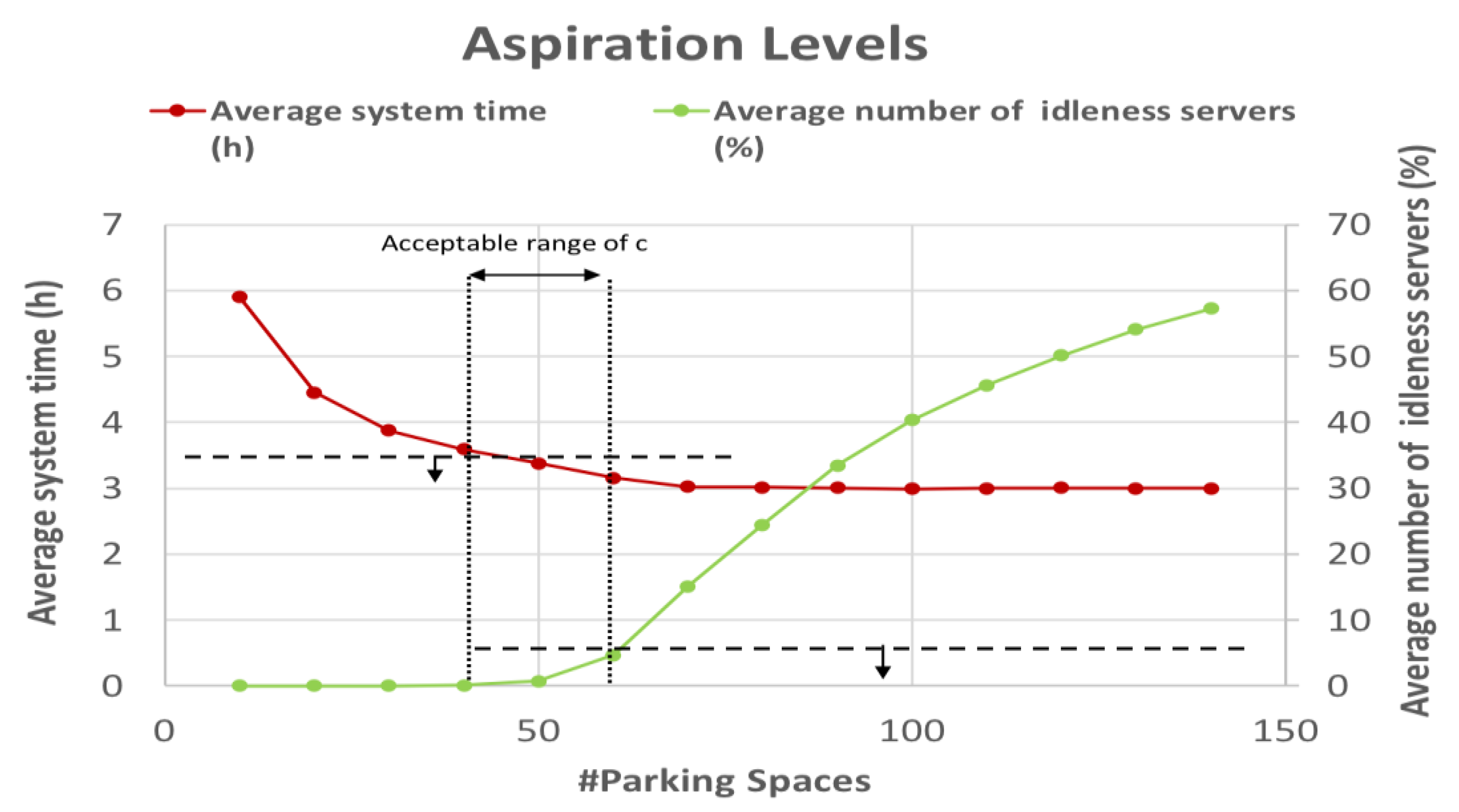
6.2.4. Selecting the Level of Service in a Parking Lot System

In general, it is possible to generate through the simulation a series of measures that can be evaluated by decision-makers for the dimensioning of an IoT system model that includes an M/M/c/N queue system. For this, we carried out a series of simulation experiments to find the optimal values of the system dimensioning. The input parameters for the simulations were λ = 20 cars/h, μ= 0.333 cars/h, and QC = 10 cars.

Table 13. Simulations of a parking lot model with an M/M/c/N queue subsystem for λ = 20 cars/h, μ = 0.333 cars/h, QC = 10 cars, and #parking spaces = c.

		Arrivals			Service			Queue		System
c	N = c + 10	Number of Arrivals (#cars)	Number of Lost Customers (#cars)	Number of Lost Customers (%)	Average Number of Busy Parking Spaces (#cars)	Average Number of Idleness Servers (%)	Average Parking Lot Utilization (%)	Average Queue Length (Lq) (#cars)	Average Waiting Time (Wq) (h)	Average System Size (Ls) (#cars)	Average System Time (Ws) (h)
10	20	100,349	83,568	83.27736201	9.999422017	0.005779828	99.99422017	9.798104615	2.921538755	19.79752663	5.903868165
20	30	99,931	66,804	66.85012659	19.99719807	0.014009667	99.98599033	9.495001551	1.432918368	29.49219962	4.452721938
30	40	100,036	49,764	49.74609141	29.99386221	0.020459301	99.9795407	8.987784398	0.893849579	38.98164661	3.877717338
40	50	100,108	33,351	33.31501978	39.95915411	0.102114716	99.89788528	8.022455748	0.600431232	47.98160986	3.593985154
50	60	100,201	17,798	17.76229778	49.61807766	0.763844672	99.236 15533	6.056626181	0.367399439	55.67470385	3.378381194
60	70	100,376	5337	5.31700805	57.16125369	4.731243856	95.26875614	2.835667889	0.148552542	59.99692157	3.154269122
70	80	99,434	366	0.368083352	59.41990667	15.11441904	84.88558096	0.359997586	0.018082026	59.77990426	3.019445625
80	90	100,177	30	0.029946994	60.42871118	24.46411102	75.53588898	0.034389131	0.001728087	60.46310031	3.016886058
90	100	99,498	0	0	59.8415345	33.50940611	66.49059389	6.03027 × 10−5	8.51719 × 10−6	59.84159481	3.005858178
100	110	99,676	0	0	59.62648983	40.37351017	59.62648983	0	0	59.62648983	2.989775325
110	120	99,717	0	0	59.75408406	45.6781054	54.3218946	0	0	59.75408406	2.997618602
120	130	99,650	0	0	59.84377321	50.13018899	49.86981101	0	0	59.84377321	3.003488982
130	140	99,378	0	0	59.66648554	54.10270343	45.89729657	0	0	59.66648554	3.002630658
140	150	99,822	0	0	59.85142554	57.24898176	42.75101824	0	0	59.85142554	2.997808869
150	160	100,078	0	0	60.07199384	59.9520041	40.0479959	0	0	60.07199384	3.002222787

shows some results obtained in each simulation that allows us to observe some variations in performance measures for various dimensions of the system (c). Figure 23 summarizes the system performance measures for some variations in the number of parking spaces using an M/M/c/N queue system with λ= 20 cars/h, μ= 0.333 cars/h, and QC = 10 cars.

Additionally, to establish an appropriate service level, the use of the aspiration level model was promoted. This model provides a balance between service level and waiting [39]. Given the experimental scope of our study, we had put aside the use of the cost model due to the difficulty of estimating waiting costs. The problem reduced to determining the number of servers c such that:

Average system time (h) ≤ a and average number of idleness servers (%) ≤ b

The constants a and b are the levels of aspiration specified by the decision-maker. We can determine an acceptable number of servers around these criteria as shown in Figure 24. For example, for a = 3.5 h and b = 5%, we had an aspiration level with an average system time (h) ≤ 3.5 and average number of idleness servers (%) ≤ 5, which resulted in a number of servers between 42 and 62.

6.2.5. Context: Simulation of the Service Operation Time of the Parking Lots in the North of a City

In this paper, we carried out a mapping of the city of Madrid, which was subdivided into four zones as shown in Figure 25. Each zone of the parking lot system was modeled and simulated with the number of parking lots required. We defined this scenario to show how to scale the simulation for various areas of a city. System simulations for an entire city could become a problem of resource performance when trying to handle large XML files. For this reason, due to the limitations of the resources of the local computer, only the simulation of the scaling of the parking lot service in the north of Madrid was performed.

This simulation was performed using two models representing the northwest and northeast areas (see Figure 26). It should be noted that it is possible to simulate the four areas of Madrid using two additional parameterized models that represent the southern area of Madrid on another computer with similar characteristics.

In the context of this scenario, the XML files (simulation-northwest.xml and simulation-northeast.xml) were parameterized and dimensioned with 15 parking lots and 9 parking lots respectively. The sensors/actuators of each model send the MQTT messages to the cloud platform at a frequency that depends on the operation of the M/M/c/N queue systems replicated in the models. For simplicity, we parameterized each of the parking lots with λ = 20 cars/h, μ = 0.333 cars/h, and queue capacity = 10 cars. Additionally, individually each parking lot was dimensioned with a specific number of parking spaces based on the current amount existing in the city of Madrid.

The details are presented in

Table 14. Simulation of T hours of operation of parking lots in the north of Madrid.

T (h)	Simulator 1 Total Number of Sensors/Actuators = 1084 (P1; P2; P3; P4; P5; P6; P7; P8; P9; P10; P11; P12; P13; P14; P15)				Simulator 2 Total Number of Sensors/Actuators = 456 (P16; P17; P18; P19; P20; P21; P22; P23; P24)
	Total Number of Messages Sent to Broker			Average of Execution Time in the Simulator (min)	Total Number of Messages sent to Broker			Average of Execution Time in the Simulator (min)
	Arrivals	Departures	Total		Arrivals	Departures	Total
100	29,482	28,610	58,092	25.62	15,296	14,849	30,145	13.34
200	59,417	58,566	117,983	41.37	30,230	29,776	60,006	24.75
300	89,252	88,358	177,610	62.06	45,228	44,772	90,000	37.96
400	118,661	117,774	236,435	79.19	59,646	59,194	118,840	47.06
500	148,068	147,111	295,179	105.64	74,892	74,436	149,328	67.31
600	178,255	177,319	355,574	126.00	90,463	90,007	180,470	79.08
700	207,914	207,007	414,921	135.52	105,113	104,657	209,770	84.22
800	237,594	236,695	474,289	156.16	120,078	119,627	239,705	95.72
900	267,082	266,189	533,271	169.40	134,243	133,789	268,032	103.87
1000	297,954	297,066	595,020	194.35	149,982	149,529	299,511	120.23

. Each of the iterations of the experiments simulates a certain number of hours of service operation. The total of MQTT messages generated in each zone and the execution time used by each of the simulators to complete the operations are provided.

Figure 27 shows the total number of messages sent by simulator-1 and simulator-2 based on the number of simulated hours of service operation. We can see that:

(a) Simulator-1 sent 595.07 messages per hour (0.165 messages per second)

(b) Simulator-2 sent 298.97 messages per hour (0.083 messages per second).

In general, given:

Y_simulator-1 = 595.07 × x + 1449.8,

(1)

Y_simulator-2 = = 298.97 × x + 149.6,

(2)

for the north of the city we had:

Z = Y_simulator-1 + Y_simulator-2 = 894.04 × x + 1599.4,

(3)

= α × x + β,

(4)

here α is the sending rate of MQTT messages to the cloud platform:

α = 0.248 messages per second

Furthermore, we can express the relationship between the effective arrival rate and the vehicle departure rate for the m parking lots in the north of the city from M/M/c/N queuing system using the following expression:

$$\mathsf{\alpha } = {\displaystyle \sum }_{\mathrm{m}=1}^{24}\left\{{\left({\mathsf{\lambda }}_{\mathrm{eff}} + \mathrm{\mu } \times \mathsf{\phi }\right)}_{\mathrm{m}}\right\}$$

(5)

here λ_eff, μ, and φ son are characteristics of each parking lot;

λ_eff: average of the effective arrival rate;

μ: average departure rate;

φ: average number of occupied parking spaces.

These proofs of concept were relevant to verify the rate of sending messages from the north of the city to the cloud platform. Taking advantage of the speed of tests through simulation, we can estimate the data loads that the system could be subjected to.

6.2.6. Context III: Simulation of Parking Lots in the North of a City in Real Time

This scenario and its parameterization were similar to that of Section 6.2.5. with the difference that the simulations were run activating the synchronization with real time. Thus, simulations were performed in a realistic way of the operation of the service, and the results and interactions with the cloud platform were analyzed.

The details are presented in

Table 15. Real-time simulation of the operation of the parking lots in the north of Madrid.

Real Time (h)	Simulator 1 Total Number of Sensors/Actuators = 1084 (P1; P2; P3; P4; P5; P6; P7; P8; P9; P10; P11; P12; P13; P14; P15)				Simulator 2 Total Number of Sensors/Actuators = 456 (P16; P17; P18; P19; P20; P21; P22; P23; P24)
	Total Number of Messages sent to Broker			Average of Execution Time in the Simulator (min)	Total Number of Messages sent to Broker			Average of Execution Time in the Simulator (min)
	Arrivals	Departures	Total		Arrivals	Departures	Total
1	303	47	350	63.98	152	20	172	62.57
5	1489	763	2252	301.33	875	459	1334	301.23
10	3082	2180	5262	605.06	1610	1164	2774	603.22
15	4478	3601	8079	903.57	2359	1905	4264	902.19
24	7079	6216	13,295	1443.97	3713	3262	6975	1442.54

. Each of the experiments simulated a certain number of real hours of service operation. Figure 28 shows the total number of messages sent by simulator-1 and simulator-2. We can observe:

(a) Simulator-1 sent 9.4597 messages per minute (0.158 messages per second);

(b) Simulator-2 sent 4.9278 messages per minute (0.0821 messages per second).

The total number of MQTT messages per second was 0.2401.

6.2.7. Model Performance of the Reservation Request Service and System’s Recovery Time in Case of Failures

The objective of this experiment was to estimate the limits of the system operations related to the simulations of the reservation requests. Additionally, we measured service recovery time when the service pod failed.

Apache JMeter was the tool used to estimate the performance of the reservation request service. Apache JMeter helped us obtain performance metrics when we made multiple concurrent requests to the microservice deployed in the cloud platform. Requests generated by Apache JMeter arrive at the reservation request microservice that communicates with the reservation allocation service. The reservation allocation service was capable of providing the reservation number and stored the results in the database.

The reservation microservices pod was deployed in the same VM where the primary replica of the database was deployed. Thus, we improved the response times of the service.

Table 16. Apache JMeter metrics of the reservation service.

Number of Threads	Ramp-Up Period	Average Throughput	Response Time			Error (%)
			Average	Minimun	Maximun
1500	60	7.8/s	71,207	8050	130,141	0.00%
2000	60	7.8/s	102,529	6313	203,920	0.00%
2000	120	7.9/s	72,774	4214	136,719	0.00%
2000	180	7.9/s	41,169	2376	79,713	0.00%
2500	180	7.9/s	72,628	3907	136,963	0.00%
10,000	3600	2.7/s	1119	1089	4218	0.00%

provides a summary of the metrics of the load tests performed with Apache JMeter. We ran the tests on a local computer that can only generate a limited total number of threads. The tests execute HTTP requests to the reservation request microservice that must collect a reservation Id from the reservation assignment service. If approximately 1500 users make reservation requests for one minute, the system can respond to these requests with an average throughput of 7.8 clients/s. For example, that average throughput can broadly satisfy reservation requests with a rate of 20 requests/hour. Figure 29 shows the behavior of the reservation service when serving 2500 users with a 180-s ramp-up.

We estimated the system’s recovery time causing failures in the Pod that contains the microservices of the reservation service. Once we caused the failure, we calculated the time it took for the Pod to return to normal operation. We executed continuous deletions of the Pod using Kubernetes commands to simulate Pod failures and observe the Pod restart time in the cloud platform. The pod restart time was on the order of milliseconds as it is a light resource.

Moreover, the recovery time of the microservices that control the reservations depends on the recovery of the state of the system (the total number of available reservations) in real time. The WSAN keeps the value of the number of available reservations, and the system recovers it by the synchronization operation when the web application restarts. Synchronization time was approximately 1 s.

7. Conclusions and Future Work

We need to have the technology layers that satisfy the requirements of an IoT application that handles cloud-based services. Thus, we can effectively simulate the scalability of an IoT system. Compared to other IoT simulators, we provide an architecture that flexibly covers the technologies layers for modeling and simulating applications with cloud-based services: WSAN modeling of IoT, the cloud layer, and the application layer. Our approach takes advantage of the technologies around cloud computing such as Kubernetes and Docker containers to achieve a more realistic simulation environment promoting the use of open source technologies. To our knowledge, IoT simulators have an underdeveloped cloud computing layer for the requirements of IoT applications.

In this article, the Ptolemy II simulation tool allowed to simulate the IoT application using the hierarchical modeling capacity of actors with certain computational models (MoC). The most important components used by Ptolemy are the MQTT-Accessors. Through the MQTT-Accessors, the Gateways of the IoT facilities based on WSANs were simulated emitting or receiving data from outside. MQTT-Accessors are components that make communication with the message broker in the cloud platform more flexible. A message broker (eMQTT) was the essential intermediary for data exchange and supporting the scalability of the IoT application. This message broker can also be used as an intermediary for other simulations of IoT applications with other scenarios, allowing the simulation of heterogeneous IoT scenarios

Another interesting feature of our design was modeling the behavior of service requests to the IoT system by end-users. Thus, we took into account the behavior of the user in the system by modeling a user layer. Thus, in the case use of the cloud-based IoT reactive parking lot system model, an M/M/c/N queuing system was implemented.

Furthermore, the Ptolemy simulator helped design WSANs in a modular and hierarchical way and helped extend the model to simulate the growth and expansion of various WSANs in large areas, such as a set of city parks. The simulation of the scalability of the IoT application was carried out with the replication of components, which helped to analyze the sizing of the system. Additionally, we could affirm that by using the simulation with a distribution of replicas of the IoT Application on several computers it is possible to accelerate the global simulation of an IoT application. Although Ptolemy facilitates hierarchical modeling and the replication of components and models, one of the limitations of our work is the inability to provide complete documentation regarding all the assumptions made about how the components were built and used.

Moreover, through cloud computing technologies, we could quickly have a minimal infrastructure to perform more realistic tests with IoT systems that have services in the cloud platform. Technologies around the cloud platform such as Kubernetes (container manager) and Docker Hub (third-party software repository) offered new opportunities to use your infrastructure.

Another of the limitations of our approach is related to the payment of services to the cloud provider. Although some cloud providers offer a free limited service for a short period, the deployed infrastructures are eliminated if we do not pay for the service. Other limitations could be prior knowledge of how Ptolomy, VisualSense, Kubernetes, and Docker work. An alternative to our design is to mount a reduced version of Kubernetes (Minikube) on one of our computers and deploy our containers on it.

Due to these results, one can envision using this approach to simulate other IoT system services. For example, the monitoring and control of bookings for reading and work areas in libraries, or the monitoring and control of bicycle rental bookings offered by a city council.

Finally, as future work, the authors will study the simulation of heterogeneous scenarios that include mobility.

References

1. Da Costa, F. Rethinking the Internet of Things: A Scalable Approach to Connecting Everything; Apress: Berkeley, CA, USA, 2013. [Google Scholar]
2. Ptolemy II Home Page. Available online: http://ptolemy.eecs.berkeley.edu/ptolemyII/ (accessed on 31 January 2021).
3. Singh, S.; Singh, N. Internet of Things (IoT): Security challenges, business opportunities & reference architecture for E-commerce. In Proceedings of the 2015 International Conference on Green Computing and Internet of Things (ICGCIoT 2015), Delhi, India, 8–10 October 2015; pp. 1577–1581. [Google Scholar] [CrossRef]
4. Chernyshev, M.; Baig, Z.; Bello, O.; Zeadally, S. Internet of Things (IoT): Research, Simulators, and Testbeds. IEEE Internet Things J. 2018, 5, 1637–1647. [Google Scholar] [CrossRef]
5. Sargent, R.G. Verification and validation of simulation models. J. Simul. 2013, 17, 12–24. [Google Scholar] [CrossRef] [Green Version]
6. Law, A.M. Simulation Modeling and Analysis, 5th ed.; McGraw-Hill: New York, NY, USA, 2014. [Google Scholar]
7. Shah, J.; Dubaria, D. Building Modern Clouds: Using Docker, Kubernetes & Google Cloud Platform. In Proceedings of the 2019 IEEE 9th Annual Computing and Communication Workshop and Conference (CCWC), Las Vegas, NV, USA, 7–9 January 2019; pp. 184–189. [Google Scholar] [CrossRef]
8. Reactive Manifesto. Available online: http://www.reactivemanifesto.org (accessed on 31 January 2021).
9. Jurado Perez, L.; Salvachua Rodriguez, J. Simulation of scalability in IoT applications. In Proceedings of the 2018 International Conference on Information Networking (ICOIN 2018), Chiang Mai, Thailand, 10–12 January 2018; pp. 577–582. [Google Scholar] [CrossRef]
10. Han, S.N.; Lee, G.M.; Crespi, N.; Heo, K.; Van Luong, N.; Brut, M.; Gatellier, P. DPWSim: A simulation toolkit for IoT applications using devices profile for web services. In Proceedings of the 2014 IEEE World Forum on Internet of Things (WF-IoT), Seoul, Korea, 6–8 March 2014; pp. 544–547. [Google Scholar] [CrossRef]
11. Gupta, H.; Dastjerdi, A.V.; Ghosh, S.K.; Buyya, R. iFogSim: A toolkit for modeling and simulation of resource management techniques in the Internet of Things, Edge and Fog computing environments. Softw. Pr. Exp. 2017, 47, 1275–1296. [Google Scholar] [CrossRef] [Green Version]
12. Zeng, X.; Garg, S.K.; Strazdins, P.E.; Jayaraman, P.P.; Georgakopoulos, D.; Ranjan, R. IOTSim: A Cloud based Simulator for Analysing IoT Applications. J. Syst. Archit. 2017, 72, 93–107. [Google Scholar] [CrossRef]
13. Sotiriadis, S.; Bessis, N.; Asimakopoulou, E.; Mustafee, N. Towards Simulating the Internet of Things. In Proceedings of the 2014 28th International Conference on Advanced Information Networking and Applications Workshops, Victoria, BC, Canada, 13–16 May 2014; pp. 444–448. [Google Scholar] [CrossRef] [Green Version]
14. Varga, A.; Hornig, R. An overview of the OMNeT++ simulation environment. In Proceedings of the 1st International Conference on Simulation Tools and Techniques for Communications, Networks and Systems & Workshops, SimuTools 2008, Marseille, France, 3–7 March 2008. [Google Scholar] [CrossRef]
15. Riley, G.F.; Henderson, T.R. The ns-3 Network Simulator. In Proceedings of the SIGCOMM’08, Seattle, WA, USA, 17–22 August 2008. [Google Scholar]
16. Lord, M.; Memmi, D. NetSim: A Simulation and Visualization Software for Information Network Modeling. In Proceedings of the 2008 International MCETECH Conference on e-Technologies (MCETECH 2008), Montreal, QC, Canada, 23–25 January 2008; pp. 167–177. [Google Scholar] [CrossRef]
17. QualNet—Network Simulation Software. Available online: https://www.scalable-networks.com/products/qualnet-network-simulation-software-tool/ (accessed on 31 January 2021).
18. Ronit, L.; Maharshi, J.; Amit, J. Survey on Network Simulators. Int. J. Comput. Appl. 2018, 182, 23–30. [Google Scholar]
19. Gandomi, A.; Tafti, V.A.; Ghasemzadeh, H. Wireless Sensor Networks Modeling and Simulation in Visualsense. In Proceedings of the 2010 Second International Conference on Computer Research and Development, Kuala Lumpur, Malaysia, 7–10 May 2010; pp. 251–254. [Google Scholar] [CrossRef]
20. VisualSense. Visual Editor and Simulator for Wireless Sensor Network Systems. Available online: https://ptolemy.eecs.berkeley.edu/visualsense/ (accessed on 31 January 2021).
21. Lee, E.A. Accessors: A Software Architecture for IoT. Talk or Presentation. 30 March 2017. Available online: https://ptolemy.berkeley.edu/projects/icyphy/pubs/73.html (accessed on 31 January 2021).
22. What Is Kubernetes?—Kubernetes. Available online: https://kubernetes.io/docs/concepts/overview/what-is-kubernetes/ (accessed on 31 January 2021).
23. What Is a Container?—App Containerization—Docker. Available online: https://www.docker.com/resources/what-container (accessed on 31 January 2021).
24. Romualdo Suzuki, L. Smart Cities IoT: Enablers and Technology Road Map. In Smart City Networks: Through the Internet of Things; Russia, S., Pardalos, P., Eds.; Springer Optimization and Its Applications; Springer: Cham, Switzerland, 2017; Volume 125, pp. 167–190. [Google Scholar] [CrossRef]
25. EMQ—The Massively Scalable Open Source MQTT Broker. Available online: http://emqtt.io/ (accessed on 31 January 2021).
26. Docker Hub. Public Image: EMQTT. Available online: https://hub.docker.com/ (accessed on 31 January 2021).
27. Apache Kafka. Available online: https://kafka.apache.org/intro (accessed on 31 January 2021).
28. The Most Popular Database for Modern Apps. Available online: https://www.mongodb.com/ (accessed on 31 January 2021).
29. Eisele, M. Developing Reactive Microservices: Enterprise Implementation in Java; O’Reilly Media Inc.: Boston, MA, USA, 2016. [Google Scholar]
30. Wolff, E. Microservices: Flexible Software Architecture; Addison-Wesley Professional: Boston, MA, USA, 2016. [Google Scholar]
31. Classic FSM—Akka Documentation. Available online: https://doc.akka.io/docs/akka/current/fsm.html (accessed on 31 January 2021).
32. EMQ 2.2—Erlang MQTT Broker: User Guide. Available online: https://emq-docs-en.readthedocs.io/en/latest/guide.html (accessed on 31 January 2021).
33. Confluent: Security. Available online: https://docs.confluent.io/platform/current/security/security_tutorial.html (accessed on 31 January 2021).
34. MongoDB Documentation: Security. Available online: https://docs.mongodb.com/manual/security/ (accessed on 31 January 2021).
35. Google Cloud: Google Infrastructure Security Design Overview. Available online: https://cloud.google.com/security/infrastructure/design/ (accessed on 31 January 2021).
36. Kubernetes: Overview of Cloud Native Security. Available online: https://kubernetes.io/docs/concepts/security/overview/ (accessed on 31 January 2021).
37. Confluent: Apache Kafka & Event Streaming Platform for the Enterprise. Available online: https://www.confluent.io/ (accessed on 31 January 2021).
38. Apache JMeter. Available online: https://jmeter.apache.org/ (accessed on 31 January 2021).
39. Taha, H.A. Operations Research: An Introduction, 10th ed.; Pearson: New York, NY, USA, 2017. [Google Scholar]
Figure 1. Modeling and simulation architecture for IoT applications in a smart city.
Applsci 11 01804 g001
Figure 2. Location of the sensors, the actuator, and the gateway in a park.
Applsci 11 01804 g002
Figure 3. Model of a wireless sensor and actuator network in a park.
Applsci 11 01804 g003
Figure 4. Model of a park in a city.
Applsci 11 01804 g004
Figure 5. General model of the reactive system.
Applsci 11 01804 g005
Figure 6. Parking lot model.
Applsci 11 01804 g006
Figure 7. Vehicle arrival/departure model based on an M/M/c/N queuing system.
Applsci 11 01804 g007
Figure 8. Main Visual Interface of the system.
Applsci 11 01804 g008
Figure 9. Reservation Request Service interface.
Applsci 11 01804 g009
Figure 10. Monitoring service.
Applsci 11 01804 g010
Figure 11. Synchronization process of the state of the parking spaces.
Applsci 11 01804 g011
Figure 12. FSM reservation allocation service.
Applsci 11 01804 g012
Figure 13. Reservation allocation service model based on an Akka FSM actor.
Applsci 11 01804 g013
Figure 14. FSM Akka actors to manage reservations in the urban center of Madrid.
Applsci 11 01804 g014
Figure 15. Location of the parks in a city.
Applsci 11 01804 g015
Figure 16. Model of the IoT application with 10 parks in a city.
Applsci 11 01804 g016
Figure 17. Experiment 1.
Applsci 11 01804 g017
Figure 18. Experiment 2.
Applsci 11 01804 g018
Figure 19. Experiment 3.
Applsci 11 01804 g019
Figure 20. Experiment 4.
Applsci 11 01804 g020
Figure 21. Message Broker.
Applsci 11 01804 g021
Figure 22. Data Monitor.
Applsci 11 01804 g022
Figure 23. Relationship between the variations of the performance measures, average queue length, average system time, and average parking lot utilization, for a parking lot model with λ= 20 cars/h, μ = 0.333 cars/h, QC = 10 cars, and #parking spaces = c.
Applsci 11 01804 g023
Figure 24. Estimation of the number of parking spaces required for a parking lot with λ = 20 cars/h, μ = 0.333 cars/h, and QC = 10 cars for aspiration level criteria: average system time (h) ≤ 3.5 and average number of idleness servers (%) ≤ 5.
Applsci 11 01804 g024
Figure 25. Modular and hierarchical distribution to model an IoT parking system for the city of Madrid.
Applsci 11 01804 g025
Figure 26. Modular and hierarchical distribution to model an IoT parking system for the north of Madrid.
Applsci 11 01804 g026
Figure 27. A linear relationship between the total number of messages sent to the cloud platform by simulators and the number of simulated hours of service operation.
Applsci 11 01804 g027
Figure 28. The relationship between the total number of messages sent to the cloud platform and the real time is linear.
Applsci 11 01804 g028
Figure 29. Throughput and response time of the reservation service behavior for 3 min.
Applsci 11 01804 g029