Abstract
Due to manufacturing errors, inaccurate measurement and working conditions changes, there are many uncertainties in laminated composite cylindrical shells, which causes the variation of vibration characteristics, and has an important influence on the overall performance. Therefore, an uncertainty representation methodology of natural frequency for laminated composite cylindrical shells is proposed, which considers probabilistic and interval variables simultaneously. The input interval variables are converted into a probabilistic density function or cumulative distribution function based on a four statistical moments method, and a unified probabilistic uncertainty analysis method is proposed to calculate the uncertainty of natural frequency. An adaptive Kriging surrogate model considering probabilistic uncertainty variables is established to accurately represent the natural frequency of laminated composite cylindrical shells. Finally, the dimensionless natural frequency of three-layer, five-layer and seven-layer laminated composite cylindrical shells with uncertainty input parameters is accurately represented. Compared with the Monte Carlo Simulation results, the mean error and standard deviation error are reduced to less than 0.07% and 4.7%, respectively, and the execution number of calculation function is significantly decreased, which fully proves the effectiveness of the proposed method.
1. Introduction
Laminated composite cylindrical shells are widely applied in aerospace, petroleum industry and ship engineering, due to their advantages of high specific strength, corrosion resistance, fatigue resistance and strong shock absorption [1,2,3]. To reveal the propagation characteristics and the inherent properties of laminated composite cylindrical shells, several determinate parameters of composite materials have been adopted [4,5]. However, due to manufacturing errors, inaccurate measurement and working condition changes in practical applications, there are many uncertainties which directly affect the basic properties of composite material [6,7]. Therefore, many uncertainty analysis methodologies are conducted to reduce the deteriorating influences of uncertainties. The uncertain properties of laminated composite cylindrical shells are mainly focused on geometric properties, elastic modulus, structural parameters, and interlayer assembly parameters. To improve the safety and durability of laminated composite cylindrical shells, it is necessary to study the vibration response characteristics of laminated composite cylindrical shells with uncertainty input parameters.
The uncertainty input variables of laminated composite cylindrical shells can be divided into aleatory uncertainties and epistemic uncertainties [8]. The aleatory uncertainties are determined by the error generated when measuring the shells’ parameters. This error can remain within a permitted range and be represented by an accurate probability density function (PDF) or cumulative distribution function (CDF). However, the uncertainty information of laminated composite cylindrical shells cannot be acquired in some engineering applications, the available uncertainty data are insufficient, making accurate uncertainty PDF unable to be acquired. The uncertainty problem produced by incorrect cognition of shells’ theory system or insufficient shells data belongs to the category of cognitive uncertainty. The epistemic uncertainties can be represented by non-probabilistic methods, such as the interval method [9,10], convex model [11,12], and fuzzy interval method [13,14,15]. However, aleatory and epistemic uncertainties coexist, which increase the complexity of uncertainty analysis of laminated composite cylindrical shells. Therefore, many methodologies of transforming cognitive uncertainty into probabilistic statistics are proposed. Zhou introduced an improved model-free sampling method based on a probabilistic weighting method to transform interval uncertainty into a probabilistic representation function. [16]. Aiming at the representation method of aleatory uncertainty and epistemic uncertainty, Zaman used flexible families of continuous Johnson distributions to represent the input interval variable [17]. Peng used the sampling analysis method to calculate the sampling interval of fourth-order moments and proposed a unified probability representation approach for multi-type uncertainties based on the cubic normal transformation method [18]. The number of input data for laminated composite cylindrical shells is often insufficient, and it is difficult to construct their accurate PDF. If the non-probabilistic representation method is conducted to solve the problem of insufficient input data, the accuracy and efficiency of natural frequency representation of laminated composite cylindrical shells can be low [19,20,21]. In the probabilistic representation method, it is very convenient to solve the mean, variance, skewness, and kurtosis in the four statistical moments method with insufficient input data, which can be represented by the likelihood continuous probabilistic measure function with high computational efficiency.
To decrease the computational complexity in uncertainty quantification of laminated composite cylindrical shells, a series of surrogate models have been proposed to replace expensive simulation models for the advantages of low computational cost and high computational accuracy. Generally, the surrogate model technology includes three basic steps: design of experiment (DOE), model construction and model validation. Rational DOE can quickly determine optimal parameter combination, effectively improve the modeling efficiency and robustness of optimization design [22,23]. To make the factor level balanced matching and the distribution of sample points more uniform, the orthogonal array, Latin hypercube sampling and optimal Latin hypercube sampling are proposed [24]. The optimal Latin hypercube sampling method can ensure that all design points are evenly distributed in the entire design space, and the spatial filling and equilibrium are stronger than other design methods, which is conductive to the construction of a surrogate model with higher accuracy [25,26]. In terms of surrogate model construction, the most common surrogate models are the response surface model (RSM) [27,28], radial basis function model (RBF) [29,30], Kriging model [31,32], artificial neural network model (ANN) [33,34], support vector regression (SVR) [35]. The Kriging model is an unbiased estimation model with the minimum approximate evaluation variance, and the distribution of function response values at unknown points can be better predicted by using the correlation function, which has faster training speed and higher accuracy than other types of surrogate models and is widely applied to replace the original objective function to solve complicated uncertainty analysis problems [36]. Dey proposed a Kriging surrogate model for analyzing the vibration characteristics of the composite shallow hyperbolic shells, which improved the calculation accuracy and efficiency compared with original Monte Carlo simulation (MCS) [37,38]. Behrooz presented an effective hybrid optimization algorithm based on the adaptive Kriging surrogate model and improved partial swarm optimization algorithm to predict the buckling characteristics of composite laminate plates [39]. Sakata used the Kriging surrogate method to analyze the random response of homogenization elastic tensor and homogenization elastic constants of unidirectional fiber reinforced composites [40,41]. Eldho studied the damage prediction of a composite plate based on the Kriging surrogate model under edge constraint conditions, and took the natural frequency and vibration change as the main research indexes, which can greatly reduce the calculation time [42]. The above literatures have verified the validity of the Kriging model acting on laminated composite plates. When the uncertain random variables and distribution parameters meet the probability distribution, it is crucial to establish the calculation method of natural frequency of laminated composite cylindrical shells based on the Kriging surrogate model. The corresponding results of the proposed method are compared with the MCS results to verify the validity of the Kriging model in laminated composite cylindrical shells [36].
In view of the uncertainty analysis problems of input variables of laminated composite cylindrical shells, the available data obtained by the experiments are converted to probabilistic variables or interval variables [43]. Using the four statistical moments method, cubic normal distribution functions are acquired, and the PDF and CDF of uncertainty input variables are transformed [18]. To increase the accuracy and computational efficiency of uncertainty analysis of natural frequency for laminated composite cylindrical shells, the uncertainty representation method for natural frequency based on the Kriging surrogate model is proposed. Considering the uncertainty of probabilistic and interval variables, the corresponding performance functions are selected to construct the initial Kriging surrogate model, and the new sample points are selected based on the maximum prediction interval criterion. The constructed Kriging surrogate model improves the accuracy of the uncertainty result and reduces the computational cost.
In general, the key scientific contribution is providing an uncertainty representation method of natural frequency for laminated composite cylindrical shells based on the four statistical moments method and the Kriging surrogate model. The main novelty of the approach is providing the conversion method from interval variables to probabilistic variables, and the uncertainty of natural frequency can be calculated using probabilistic uncertainty analysis methods, and the accuracy of uncertainty analysis results is improved through using the proposed adaptive Kriging model. The rest of this paper is organized as follows. In Section 2, considering many uncertain variables, the natural frequency calculation method of laminated composite cylindrical shells is described. In Section 3, The four statistical moments method is proposed to convert interval variables of laminated composite cylindrical shells to PDF and CDF. In Section 4, based on the maximization criterion of the target prediction interval, the Kriging surrogate model for laminated composite cylindrical shells with uncertain input variables is presented. In Section 5, the step-by-step procedure of representing the natural frequency uncertainty of laminated composite cylindrical shells is given. In Section 6, Some examples are conducted to verify the correctness and effectiveness of the proposed method. In Section 7, the conclusions are presented.
2. Problem Description
In this research, the laminated composite cylindrical shells of T300/QY8911 are studied. Due to the vibration characteristics of composite materials being different from that of isotropic structures, the natural frequency is considered as the performance objective function to investigate the vibration characteristics of laminated composite cylindrical shells [44].
The uncertainty factors of laminated composite cylindrical shells mainly include elastic modulus, shell thickness, dimension parameters and strength coefficient. To simplify the problem, some elastic modulus parameters, including the modulus of longitudinal elasticity , the transverse modulus of elasticity , the main and secondary Poisson ratio and , and in-plane shear modulus G, are considered to be uncertain. In addition, other parameters, such as the shell thickness h, the radius of middle surface R, shell density , shell length X and the number of layers L are assumed as determinate [8]. When the above parameters are determined, the solving method of natural frequency of laminated composite cylindrical shells becomes a difficulty [45]. Therefore, the solving method of natural frequency is discussed as follows.
First, based on the Love shell theory, the free vibration equations of laminated composite cylindrical shells are acquired [46]. Considering the coupling effect, the vibration characteristics of laminated composite cylindrical shells with different laying were studied [47]. According to the Love shell theory, the middle surface micro-element at laminated cylindrical shells was taken as the research object. The acting forces and moments on the micro-element are shown in Figure 1. , and represent the radial, circumferential, and axial of laminated composite cylindrical shells in cylindrical coordinates. , and represent internal force on a micro plane, , and represent internal moment on a micro plane, , and represent the axial, circumferential and radial displacement of middle surface of cylindrical shells [48,49].
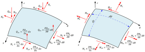
Figure 1.
The force and moment distribution of laminated composite cylindrical shells.
Therefore, the differential equations of free vibration of the laminated composite cylindrical shells are expressed as
where the forces and moments of laminated composite cylindrical shells are described by
where , and are the micro-element stress in different directions. According to the generalized Hooke’s law, the stress in Equation (2) can be expressed as
The coefficient (ij = 11, 12, 22, 66) is the reduction stiffness matrix coefficient of monolayer composite materials, where , , and . , and are the axial, circumferential and shear strains at the distance from the reference Z-place. The relationship between the main and secondary Poisson ratios is . Based on the Love shell model, the strains are expressed as , and , where , and are reference surface strain, , and are reference surface strain curvature. The reference surface strain and curvature are expressed as
By substituting Equation (4) into Equation (2), the internal force of the cylindrical shells can finally be expressed as the following matrix form:
where , and are the tensile stiffness, coupling stiffness and bending stiffness, which are the key factors in representing the natural frequency of different ply angles of laminated composite cylindrical shells. The tensile stiffness, coupling stiffness and bending stiffness are expressed as
Due to the research object being the symmetrical layering of cylindrical shells, Bij is generally calculated as 0. Assuming that , , and , represents the ply angle of laminated composite cylindrical shells. The partial axis stiffness coefficient of the kth layer is described by
where Si(i = 1, 2, 3, 4) is the conversion coefficient, which can be solved by
Considering coupling between circumferential and axial modes, the free vibration of laminated composite cylindrical shells propagates in the way of waves, so the surface displacement of the shells can be expressed as the following by wave propagation method [50]:
where , and are the amplitude in the , and directions, is the axial wave number, m and n are the axial and circumferential mode orders, is the circular frequency. For the different boundary conditions, there are different ways to calculate the axial wave number , which can use the calculation method of the axial wave number in the beam model to approximate the axial wave number in composite layered cylindrical shells [51]. The axial wave numbers under different boundary conditions are given in the Table 1.

Table 1.
The calculation method of the axial wave number under different boundary conditions.
By substituting Equation (9) into Equation (1), the differential equation of free vibration of the laminated composite cylindrical shells can be expressed as:
The concrete expressions of the matrix are described as:
where represents the dimensionless natural frequency (DNF) of the laminated composite cylindrical shells, which can be calculated by . When the composite material is determined, there is only a proportional relationship between the DNF and the natural frequency. Therefore, the DNF can be used to replace the natural frequency to represent. To give a non-zero solution, the determinant of coefficient matrix must be 0.
The DNF of laminated composite shells with finite length can be obtained by solving the coefficient matrix, and the determinant is transformed into an algebraic equation of DNF, which can be expressed as
where are the coefficients of an algebraic equation of DNF, which are the functions of radius, thickness, longitudinal elastic modulus, transverse elastic modulus, Poisson’s ratio, ply angle and other parameters. By observing Equation (13), it can be found that there are three pairs of characteristic roots, including three positive roots and three negative roots, for each natural frequency. The three positive roots, respectively, represent the free vibration frequency of the axial, circumferential and radial of the laminated composite cylindrical shells, where the minimum positive root corresponds to bending vibration, and the other two positive roots correspond to in-plane vibration [52].
After the natural frequency equations of laminated composite cylindrical shells are acquired successfully, based on the four statistic moments method, the probabilistic variables and interval variables of various uncertain input parameters are transformed to PDF and, according to the optimal Latin hypercube sampling method and the Kriging surrogate model, the natural frequency of laminated composite cylindrical shells with uncertainty input parameters is represented.
3. Interval and Probabilistic Variables Conversion Based on the Four Statistical Moments Method
In Section 2, the modulus of longitudinal elasticity , the transverse modulus of elasticity , the main and secondary Poisson ratio and , and in-plane shear modulus G are considered as the uncertainty variables. According to the available information of input data, these uncertainty variables can be divided into probabilistic variables and interval variables, which need to be solved by different uncertainty methods. Therefore, to unify the uncertainty analysis method, the interval and probabilistic variables conversion method based on the four statistical moments method is proposed [18].
For the probabilistic variables, the PDF value of the sampling points can be easily obtained, so the four statistical moments (mean , variance , skewness , kurtosis ) can be directly calculated, as shown in Equation (14).
Among them, according to the ns random discrete sampling points of the statistical variables and the corresponding PDF value , the 1–4 order statistical moments can be directly calculated by
For the interval variables, the PDF value of these sampling points is not available, and the exact PDF of interval variables is difficult to obtain. In the uncertainty design domain, the number and location of selected sampling points are different, and the calculated value of the 1–4 order statistical moments will also be variable. Therefore, its four statistical moments are an uncertainty interval . The upper and lower bounds of the interval are calculated by using the optimization function of Equation (16).
First, sample uniformly within the uncertainty interval of interval variables to obtain ns sampling points . Then the PDF value of each sampling point is used as the optimization variable, and is optimized within the variable interval of the uncertainty variables to determine the upper and lower bounds of the interval . For example, if the interval variable x is an interval variable represented by a single interval method, the PDF value of each sampling point is a random number in the range of (0, 1), and the total PDF value of the random sampling points is 1.
According to the four statistical moments of interval variable x, the standardized variable is transformed into the cubic function of random variable , as shown in Equation (17).
where the mean value is solved by , standard deviation is solved by , and the coefficients of the cubic function are functions of the four statistical moments , and the specific calculation details can be found in Ref. [17].
After determining the coefficient values , the random variable can be classified by the values of , and . The specific division method is shown in Table 2. The six types include unbounded distribution types (Type I and Type VI), unilaterally bounded distribution types (Type II, Type IIII, and Type V), and bilaterally bounded distribution types (Type IV). The definitions of parameters and can be found in the literature [53,54].
Table 2.
The division criterion of standardized transformation random variable
According to the transformed PDF of the random variable , the PDF value of the interval variable x is calculated by Equation (18), to realize the probabilistic conversion of the interval variables.
4. Construction of Accurate Kriging Model Based on Prediction Interval Criterion
4.1. The Basic Principle of Kriging Model
The Kriging surrogate model adopts the Gaussian random process model, which is an internal interpolation technology based on mathematical statistics, reflecting the approximate function relationship between the object and the problem [55]. The interpolation result is defined as the linear weighting of the response value of the known sample function, which is composed of a parametric model and a nonparametric random model [56]. The former is mainly used to simulate the global approximation of the real model, while the latter mainly provides the approximate local deviation, which are described as
where is the regression function, is the polynomial function, is the error obeying random distribution , and the covariance is expressed as
where is the correlation equation of any two sampling points and , which plays a decisive role in the fitting accuracy of the Kriging surrogate model. The mean and mean square deviation of the Kriging surrogate model at prediction points are solved by
where mean square deviation represents the magnitude of model uncertainty at the measuring point to be measured.
4.2. The Proposed Improved Kriging Model
After transforming interval variables and probabilistic variables into PDF, an accurate Kriging model is constructed, where the sampling points are selected based on the maximization criterion of the performance target prediction interval, the balance between modeling efficiency and model robustness is achieved by increasing the sampling points of uncertain variables and reducing the uncertainty of the performance response.
According to the mean value and mean square error of the Kriging surrogate model at the prediction point , the prediction interval of the performance target is determined by the rule as .
Aiming at the optimization design problem with the minimum of natural frequency, the initial Kriging model is constructed according to the existing sampling points, and the optimal value of the uncertainty variable is calculated with the objective of minimum of natural frequency. The upper bound of the performance prediction at the optimal value is , and the lower bound of the prediction interval based on any other input variable is . Then a new sampling point is selected based on the criterion of maximizing the prediction interval, the new input variable is the corresponding input variable when the following function takes the maximum value, where it can be expressed by
Step 1: sampling the initial sample points. Assuming that the uncertain input variables and the distribution parameters all obey the random normal distribution, the optimal Latin hypercube method in DOE is used for uniform sampling to obtain the initial set of m sampling points.
Step 2: construction of the initial Kriging surrogate model. Using computer numerical analysis, the output response values corresponding to each sample point are calculated. The initial Kriging surrogate model based on the m sampling points and response values of uncertain variables is constructed to obtain the predicted mean and predicted variance function of the Kriging model.
Step 3: the solution of the optimal input variables based on the Kriging model . Taking the minimum natural frequency response as the objective, the corresponding sampling points in the model are selected as the optimal input variables, and the upper and lower bounds of the prediction interval are obtained.
Step 4: the selection of new sampling points. Based on the maximization criterion of the prediction interval, according to Equation (23), the (m + 1)th sampling point is sampled and the corresponding output response values of these m + 1 sampling points are solved to construct a new Kriging model.
Step 5: iteration termination criterion. In the iterative process, when the error between the surrogate model updated by the two samplings before and after is less than the set value , the iteration is stopped. Assuming that the Kriging model for the first sampling is , the model built after adding sampling points is , and the error function expressions of the two Kriging models before and after are:
The termination criterion of the Kriging surrogate model is shown in Equation (25). The value of is determined by the initial model determined in step 2, and generally takes 0.001.
5. Uncertainty Measurement of Natural Frequency
The above sections only describe the basic principles of the four statistical moments method and Kriging surrogate model, which are not introduced into engineering examples. The natural frequency analysis process of the laminated composite cylindrical shells based on the four statistical moments method and the Kriging surrogate model with insufficient available data of uncertain input parameters is listed below.
Step 1. Uncertainty transformation of interval variables. According to the amount and information of data input, the uncertain input parameters can be divided into probabilistic variables and interval variables. Since the data amount of uncertain input parameters of laminated composite cylindrical shells is smaller, the interval variables account for more than half of all uncertain variables, and it is difficult to obtain accurate PDF, so the uncertain transformation of interval variables becomes the research focus.
Step 2. Uncertainty measurement of probabilistic and interval variables. Probabilistic variables can be directly converted into PDF through sampling data. In the uncertainty interval of interval variables, the ns sampling points are obtained by uniform sampling, and the PDF value of each sampling point is used as the optimization variable. The four statistical moments of interval variables are obtained to convert into a cubic normal distribution function according to the corresponding conversion method. Finally, according to the partition criterion of standardized transformed random variables , the PDF of interval variables is acquired by Equation (18).
Step 3. Probabilistic and interval variables sampling, and performance value calculation at sampling points. After the operation of step 2, the uncertain input variables of the laminated composite cylindrical shells all obey the random normal distribution, and the optimal Latin hypercube method is used for uniform sampling to obtain the initial set of m sampling points.
Step 4. Kriging surrogate model construction and the optimal input variables solution. Using numerical calculation software, the natural frequency of the laminated composite cylindrical shells corresponding to each sampling point is obtained. Based on the sampling points of the uncertain input variables and the natural frequency calculation values, the initial Kriging surrogate model is constructed to acquire the predicted mean and predicted variance functions. Taking the minimum natural frequency response as the objective, the upper and lower bounds of the prediction interval are acquired.
Step 5. The adaptive increase in sampling points. Based on the prediction interval maximization criterion, according to Equation (19), the new sampling point and the corresponding natural frequency are obtained to construct the new Kriging surrogate model.
Step 6. Uncertainty representation of natural frequency based on the Kriging surrogate model. The error of the corresponding natural frequency is calculated by Equation (24), and the error mean is shown in Equation (25). If the error mean is less than the set value , the sampling is stopped, that is, the natural frequency of the laminated composite cylindrical shells with uncertain input variables is accurately represented. Otherwise, step 5 is performed again until the natural frequency is accurately represented.
6. Numerical Examples
To verify the correction of the proposed method, many numerical cases of laminated composite cylindrical shells with different layers and different boundary conditions are implemented to study the accurate representation of the natural frequency of laminated composite shells with different uncertain input variables.
6.1. Construction of Accurate Kriging Model
Due to a series of errors during manufacturing and installation, some uncertain factors are generated. In Section 2, the longitudinal modulus of elasticity , the transverse modulus of elasticity , the main and secondary Poisson ratio and , and in-plane shear modulus G are considered to be uncertain, The material of laminated composite cylindrical shells is T300/QY8911. The length X, radius R, thickness h and density of laminated composite cylindrical shells are 1000, 1000, 100 mm and 1380 kg/m3. The uncertainty parameters of composite laminated cylindrical shells can change the matrix coefficients in Equation (3), which can affect the subsequent DNF calculations. Therefore, the uncertain parameters are classified, and then the interval variables are converted into the corresponding CDFs by using the four statistical moments method, which can facilitate the subsequent calculation. The available data for the uncertain input variables are listed in Table 3, and these data are the partial data from Ref. [57].
Table 3.
Uncertain available data for laminated composite cylindrical shells.
According to the available uncertainty data of laminated composite cylindrical shells, the probabilistic variables are and G, and the interval variables are and . The classification details and methods of uncertain variables are found in Ref. [57]. The Poisson ratio obeys normal probability distribution, where the mean and variance are 0.329 and 0.146, respectively. The in-plane shear modulus G also obeys normal probability distribution, where the mean and variance are 5.145 and 0.3, respectively. Due the longitudinal modulus of elasticity and the longitudinal modulus of elasticity not being able to constitute an accurate PDF, it is necessary to convert the available data into interval variables for calculation. The upper bounds and lower bounds of the interval variables can be solved by
where and are the maximum and minimum values of all the sampling points, is the standard deviation, and is the tolerance coefficient. Generally, the standard deviation is set as 0.4 [58]. Therefore, the interval variables of and are and , respectively. Then the interval variables are transformed into cubic normal distribution PDF by the four statistic moments method, and the CDF of interval variables and are shown in Figure 2.
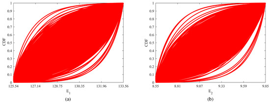
Figure 2.
Cumulative probability density functions of interval variables (a) , (b) .
6.2. Three-Layer Laminated Composite Cylindrical Shells
The proposed method is applied to the accurate representation of the natural frequency of three-layer laminated composite cylindrical shells with each ply angle , where the range of θ is from 0 to π/2. Each layer of laminated composite cylindrical shells is uniformly distributed, that is the thickness of each layer is h/L = 0.033 m. When the cubic normal PDF of uncertain input variables is determined, the optimal Latin hypercube is needed for uniform sampling. To ensure the computational efficiency and the effectiveness of the proposed method, the six sampling points are first selected for each uncertain input variable to construct the initial Kriging model. Then, according to the method described in the Section 5, the accurate Kriging model is constructed to accurately represent the frequency uncertainty for laminated composite cylindrical shells. Finally, the MCS method is adopted to replace the real calculation model and is compared with the initial Kriging and accurate Kriging methods. The mean and standard deviation of DNF for laminated composite cylindrical shells under different boundary conditions are shown in Figure 3 and Figure 4.
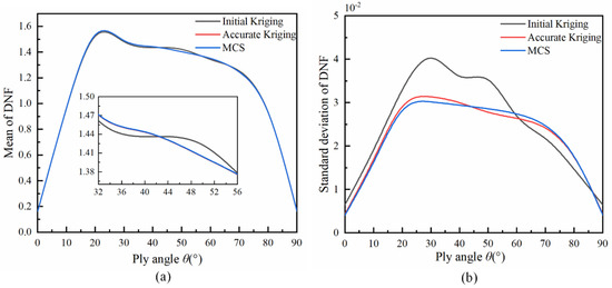
Figure 3.
The mean and standard deviation of DNF for the three-layer laminated composite cylindrical shells with clamped–clamped boundary conditions. (a) mean, (b) standard deviation.
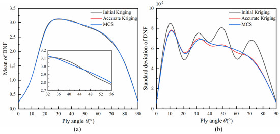
Figure 4.
The mean and standard deviation of DNF for the three-layer laminated composite cylindrical shells with supported–supported boundary conditions. (a) mean, (b) standard deviation.
By calculating the error, the maximum relative mean error and standard deviation error of DNF for the laminated composite cylindrical shells with clamped–clamped boundary conditions are reduced to 0.05% and 6.85%, respectively. In a similar way, the maximum relative mean error and standard deviation error of DNF for the laminated composite cylindrical shells with supported–supported boundary conditions are reduced to 0.05% and 4.07%. Therefore, the DNF curves obtained by the accurate Kriging method are highly fitted with the curve obtained by the MCS method, which fully proves the effectiveness of the proposed method. At the moment, the calculation number of the DNF for the laminated composite cylindrical shells reduces from 10,000 to 1000, which exhibits the proposed method has high calculation efficiency. In general, the accurate Kriging model can be applied to the accurate representation of the uncertain natural frequency of laminated composite cylindrical shells with the other boundary conditions.
6.3. Five-Layer and Seven-Layer Laminated Composite Cylindrical Shells
The proposed method also is adopted to accurately represent the natural frequency of five-layer laminated composite cylindrical shells with each ply angle and seven-layer laminated composite cylindrical shells with each ply angle under the clamped–supported boundary conditions, where the ply angle is . The mean and standard deviation of the initial Kriging model, accurate Kriging model and MCS for the five-layer and seven-layer laminated composite cylindrical shells are shown in the Figure 5 and Figure 6. The maximal relation error of the mean and standard deviation of DNF for the five-layer and seven-layer laminated composite cylindrical shells are reduced to 0.07%, 0.07%, 4.67% and 4.7%, respectively. These errors are highly similar with the maximum relative mean error and standard deviation error of DNF under clamped–clamped boundary conditions, which indicates the correction of the accurate Kriging model.
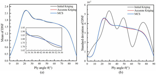
Figure 5.
The mean and standard deviation of DNF for the five-layer laminated composite cylindrical shells with clamped–supported boundary conditions. (a) mean, (b) standard deviation.
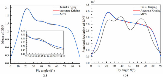
Figure 6.
The mean and standard deviation of DNF for the seven-layer laminated composite cylindrical shells with clamped–supported boundary conditions. (a) mean, (b) standard deviation.
7. Conclusions
To accurately represent the natural frequency of laminated composite cylindrical shells with probabilistic and interval variables, the uncertain representation method based on the four statistical moments and accurate Kriging surrogate models is proposed. The uncertain input parameters obtained in the experiment are converted into probabilistic and interval variables. Based on the four statistic moments method, the probabilistic cubic normal distribution functions are constructed and, according to standardized partition criteria for transforming the random variables, the PDF and CDF of interval variables are calculated. Subsequently, the optimal Latin hyper method is used to uniformly sample the interval variables and obtain the corresponding natural frequency to form the initial Kriging surrogate model. Finally, combined with the prediction interval maximization criterion, the sampling points are adaptively increased to establish to the accurate Kriging surrogate model, which can accurately represent the natural frequency of laminated composite cylindrical shells with uncertain input variables. The proposed method and MCS method are conducted to calculate the uncertain natural frequency of laminated composite cylindrical shells with different boundary conditions and different layers, and these results are highly fitting. In addition, the proposed method can greatly reduce the execution number of calculation functions and improve calculation efficiency.
Although the proposed method can accurately represent the uncertain natural frequency of laminated composite cylindrical shells, there are some limitations for solving some engineering examples, which can be further studied: (1) the types of uncertain variable should be varied according to the amount and information of available input data. When the amount of input data increases, the interval variables can be transformed into the probabilistic variables, where the probabilistic variables can simplify the algorithm with very little calculation. Therefore, the accurate representation method of natural frequency should be adaptively adjusted when the input number of uncertain parameters changes. (2) The proposed uncertainty representation method is applicable to inherent characteristic of laminated composite cylindrical shells, such as natural frequency. However, there are many external excitations and the proposed method is no longer applicable. Therefore, the further research required is to represent the response characteristics and vibration propagation law of laminated composite cylindrical shells with different boundary conditions under the external excitation of uncertain input variables.
Author Contributions
The individual contributions of authors are specified as follows. Conceptualization, G.C. and X.P.; methodology, X.P.; software, T.W.; validation, T.W., C.L. and Y.Y.; formal analysis, T.W.; investigation, L.L.; resources, X.P.; data curation, Z.Y.; writing—original draft preparation, T.W. and G.C.; writing—review and editing, T.W.; visualization, Y.Y.; supervision, G.C.; project administration, X.P. and C.L.; funding acquisition, C.L. All authors have read and agreed to the published version of the manuscript.
Funding
This research was funded by National Natural Science Foundation of China (Grant No. 51775501, 51775510, 51875525) and Natural Science Foundation of Zhejiang province (Grant No. LZ21E050003, LY21E050008).
Institutional Review Board Statement
Not applicable.
Informed Consent Statement
Not applicable.
Data Availability Statement
Data sharing not applicable.
Conflicts of Interest
The authors declare no conflict of interest.
References
- Alankaya, V.; Alarcin, F. Using sandwich composite shells for fully pressurized tanks on liquefied petroleum gas carriers. Stroj. Vestn. J. Mech. Eng. 2016, 62, 32–40. [Google Scholar] [CrossRef]
- Cao, X.T.; Ma, C.; Hua, H.X. Acoustic radiation from thick laminated cylindrical shells with sparse cross stiffeners. J. Vib. Acoust. 2013, 135, 031009. [Google Scholar] [CrossRef]
- Qi, H.; Qin, S.K.; Cheng, Z.C.; Teng, Q.; Hong, T.; Yi, X. Towards understanding performance enhancing mechanism of micro-holes on K9 glasses using ultrasonic vibration-assisted abrasive slurry jet. J. Manuf. Process. 2021, in press. [Google Scholar]
- Lam, K.Y.; Qian, W. Free vibration of symmetric angle-ply thick laminated composite cylindrical shells. Compos. Part B Eng. 2000, 31, 145–154. [Google Scholar] [CrossRef]
- Liu, C.C.; Li, F.M.; Huang, W.H. Transient wave propagation and early short time transient responses of laminated composite cylindrical shells. Compos. Struct. 2011, 93, 2587–2597. [Google Scholar] [CrossRef]
- Tomar, S.S.; Zafar, S.; Talha, M.; Gao, W.; Hui, D. State of the art of composite structures in non-deterministic framework: A review. Thin Walled Struct. 2018, 132, 700–716. [Google Scholar] [CrossRef]
- Tan, D.P.; Li, L.; Zhu, Y.L.; Zheng, S.; Yin, Z.C.; Li, D.F. Critical penetration condition and Ekman suction-extraction mechanism of sink vortex. J. Zhejiang Univ. Sci. A 2019, 20, 61–72. [Google Scholar] [CrossRef]
- Peng, X.; Guo, Y.L.; Qiu, C.; Wu, H.P.; Li, J.Q.; Chen, G.H.; Jiang, S.F.; Liu, Z.Y. Reliability optimization design for composite laminated plate considering multiple types of uncertain parameters. Eng. Optimi. 2021, 53, 221–236. [Google Scholar] [CrossRef]
- Cheng, J.; Liu, Z.Y.; Tang, M.Y.; Tan, J.R. Robust optimization of uncertain structures based on normalized violation degree of interval constraint. Comput. Struct. 2017, 182, 41–54. [Google Scholar] [CrossRef]
- Hurtado, J.E.; Alvarez, D.A.; Paredes, J.A. Interval reliability analysis under the specification of statistical information on the input variables. Struct. Saf. 2017, 65, 35–48. [Google Scholar] [CrossRef]
- Ben-Haim, Y. A non-probabilistic concept of reliability. Struct. Saf. 1994, 14, 227–245. [Google Scholar] [CrossRef]
- Ni, B.Y.; Jiang, C.; Huang, Z.L. Discussions on non-probabilistic convex modelling for uncertain problems. Appl. Math. Model. 2018, 59, 54–85. [Google Scholar] [CrossRef]
- Shao, S.T.; Zhang, X.H.; Li, Y.; Bo, C.X. Probabilistic single-valued (interval) neutrosophic hesitant fuzzy set and its application in multi-attribute decision making. Symmetry 2018, 10, 419. [Google Scholar] [CrossRef]
- Li, L.; Qi, H.; Yin, Z.C.; Li, D.F.; Zhu, Z.L.; Viboon, T.; Tan, D.P. Investigation on the multiphase sink vortex Ekman pumping effects by CFD-DEM coupling method. Powder Technol. 2020, 360, 462–480. [Google Scholar] [CrossRef]
- Wang, C.; Qiu, Z.Q.; He, Y.Y. Fuzzy interval perturbation method for uncertain heat conduction problem with interval and fuzzy parameters. Int. J. Numer. Methods Eng. 2015, 104, 330–346. [Google Scholar] [CrossRef]
- Zhou, C.C.; Tang, C.H.; Liu, F.C.; Wang, W.X. A probabilistic representation method for interval uncertainty. Int. J. Comp. Meth. Sing. 2018, 15, 1850038. [Google Scholar] [CrossRef]
- Zaman, K.; Rangavajhala, S.; McDonald, M.P.; Mahadevan, S. A probabilistic approach for representation of interval uncertainty. Reliab. Eng. Syst. Saf. 2011, 96, 117–130. [Google Scholar] [CrossRef]
- Peng, X.; Gao, Q.L.; Li, J.Q.; Liu, Z.Y.; Yi, B.; Jian, S.F. Probabilistic representation approach for multiple types of epistemic uncertainties based on cubic normal transformation. Appl. Sci. 2020, 10, 4698. [Google Scholar] [CrossRef]
- Li, L.; Lu, J.F.; Fang, H.; Yin, Z.C.; Wang, T.; Wang, R.H.; Fan, X.H.; Zhao, L.J.; Tan, D.P.; Wan, Y.H. Lattice Boltzmann method for fluid-thermal systems: Status, hotspots, trends and outlook. IEEE Access 2020, 8, 27649–27675. [Google Scholar] [CrossRef]
- Lu, J.F.; Wang, T.; Li, L.; Yin, Z.C.; Wang, R.H.; Fan, X.H.; Tan, D.P. Dynamic characteristics and wall effects of bubble bursting in gas-liquid-solid three-phase particle flow. Processes 2020, 8, 760. [Google Scholar] [CrossRef]
- Peng, X.; Li, D.H.; Wu, H.P.; Liu, Z.Y.; Li, J.Q.; Jiang, S.F.; Tan, J.R. Uncertainty analysis of composite laminated plate with data-driven polynomial chaos expansion method under insufficient input data of uncertain parameters. Comput. Struct. 2019, 209, 625–633. [Google Scholar] [CrossRef]
- Yin, Z.C.; Lu, J.F.; Li, L.; Wang, T.; Wang, R.H.; Fan, X.H.; Lin, H.K.; Huang, Y.S.; Tan, D.P. Optimized scheme for accelerating the slagging reaction and slag-metal-gas emulsification in a basic oxygen furnace. Appl. Sci. 2020, 10, 5101. [Google Scholar] [CrossRef]
- Hu, X.X.; Xu, F.; Wang, R.H.; Tan, D.P. Synchronous sampling-based direct current estimation method for self-sensing active magnetic bearings. Sensors 2020, 20, 3497. [Google Scholar] [CrossRef]
- Ma, P.; Zhou, P.C.; Shang, X.B.; Yang, M. Firing accuracy evaluation of electromagnetic railgun based on multicriteria optimal Latin hypercube design. IEEE Trans. Plasma Sci. 2017, 45, 1503–1511. [Google Scholar] [CrossRef]
- Wang, J.X.; Tan, D.P.; Cao, B.; Fan, J.; Deep, S. An independent path-based process recommendation algorithm for improving biomedical process modeling. Electron. Lett. 2020, 56, 531–533. [Google Scholar] [CrossRef]
- Wang, J.X.; Cao, B.; Zheng, X.; Tan, D.P.; Fan, J. Detecting difference between process models using edge network. IEEE Access 2019, 7, 142916–142925. [Google Scholar] [CrossRef]
- Buyukada, M. Probabilistic uncertainty analysis based on Monte Carlo simulations of co-combustion of hazelnut hull and coal blends: Data-Driven modeling and response surface optimization. Bioresour. Technol. 2017, 225, 106–112. [Google Scholar] [CrossRef]
- Yadav, R.N. A hybrid approach of Taguchi-Response surface methodology for modeling and optimization of duplex turning process. Measurement 2017, 100, 131–138. [Google Scholar] [CrossRef]
- Tan, D.P.; Li, L.; Zhu, Y.L.; Zheng, S.; Ruan, H.J.; Jiang, X.X. An embedded cloud database service method for distributed industry monitoring. IEEE Trans. Ind. Inform. 2018, 14, 2881–2893. [Google Scholar] [CrossRef]
- Fantuzzi, N.; Bacciocchi, M.; Tornabene, F.; Viola, E.; Ferreira, A.J.M. Radial basis functions based on differential quadrature method for the free vibration analysis of laminated composite arbitrarily shaped plates. Compos. Part B Eng. 2015, 78, 65–78. [Google Scholar] [CrossRef]
- Freier, L.; Wiechert, W.; von Lieres, E. Kriging with trend functions nonlinear in their parameters: Theory and application in enzyme kinetics. Eng. Life Sci. 2017, 17, 916–922. [Google Scholar] [CrossRef]
- Tan, D.P.; Li, L.; Yin, Z.C.; Li, D.F.; Zhu, Y.L.; Zheng, S. Ekman boundary layer mass transfer mechanism of free sink vortex. Int. J. Heat Mass Trans. 2020, 150, 119250. [Google Scholar] [CrossRef]
- Wang, J.Y.; Zhang, C. Software reliability prediction using a deep learning model based on the RNN encoder-decoder. Reliab. Eng. Syst. Saf. 2018, 170, 73–82. [Google Scholar] [CrossRef]
- Zhang, X.W.; Liu, J.X.; Chen, X.F.; Cao, H.R. Neural network based multi-objective active vibration optimization method for shell structure. Chin. J. Mech. Eng. Engl. 2016, 52, 56–64. [Google Scholar] [CrossRef]
- Abibullaev, B.; An, J.; Jin, S.-H.; Lee, S.H.; Moon, J. Minimizing inter-subject variability in fNIRS-based brain-computer interfaces via multiple-kernel support vector learning. Med. Eng. Phys. 2013, 35, 1811–1818. [Google Scholar] [CrossRef]
- Mukhopadhyay, T.; Chakraborty, S.; Dey, S.; Adhikari, S.; Chowdhury, R. A critical assessment of Kriging model variants for high-fidelity uncertainty quantification in dynamics of composite shells. Arch. Comput. Methods Eng. 2017, 24, 495–518. [Google Scholar] [CrossRef]
- Tan, D.P.; Zhang, L.B.; Ai, Q.L. An embedded self-adapting network service framework for networked manufacturing system. J. Intell. Manuf. 2019, 30, 539–556. [Google Scholar] [CrossRef]
- Dey, S.; Mukhopadhyay, T.; Adhikari, S. Stochastic free vibration analyses of composite shallow doubly curved Shells—A Kriging model approach. Compos. Part B Eng. 2015, 70, 99–112. [Google Scholar] [CrossRef]
- Behrooz, K.; Trung, N.; Tam, T.; Zhu, S.P. Optimization of buckling load for composite laminated plates using adaptive Kriging-improved PSO: A novel hybrid intelligent method. Def. Technol. 2021, 17, 85–99. [Google Scholar]
- Sakata, S.; Ashida, F.; Zako, M. Kriging-Based approximate stochastic homogenization analysis for composite materials. Comput. Methods Appl. Mech. 2007, 197, 1953–1964. [Google Scholar] [CrossRef]
- Pan, Y.; Ji, S.M.; Tan, D.P. Cavitation based soft abrasive flow processing method. Int. J. Adv. Manuf. Technol. 2020, 109, 2587–2602. [Google Scholar] [CrossRef]
- Eldho, J.J.; Arjun, S.; Menon, N.; Biju, N. Implementation of kriging surrogate models for delamination detection in composite structures. Adv. Compos. Lett. 2018, 27, 220–231. [Google Scholar]
- Jiang, Q.S.; Tan, D.P.; Li, Y.B.; Ji, S.M.; Cai, C.P.; Zheng, Q.M. Object detection and classification of metal polishing shaft surface defects based on convolutional neural network deep learning. Appl. Sci. 2020, 10, 87. [Google Scholar] [CrossRef]
- Yang, J.H.; Fu, Y.M. Analysis of dynamic stability for composite laminated cylindrical shells with delaminations. Comput. Struct. 2007, 78, 209–315. [Google Scholar] [CrossRef]
- Ge, J.Q.; Li, C.; Gao, Z.Y.; Ren, Y.L.; Xu, X.S.; Li, C.; Xie, Y. Softness abrasive flow polishing method using constrained boundary vibration. Powder Technol. 2021, 382, 173–187. [Google Scholar] [CrossRef]
- Lam, K.Y.; Loy, C.T. Analysis of rotating laminated cylindrical shells by different thin shell theories. J. Sound Vib. 1995, 196, 23–35. [Google Scholar] [CrossRef]
- Wu, M.G.; Lu, C.D.; Tan, D.P.; Hong, T.; Chen, G.H.; Wen, D.H. Effects of metal buffer layer for amorphous carbon film of 304 stainless steel bipolar plate. Thin Solid Films 2016, 616, 507–514. [Google Scholar]
- Tan, D.P.; Ni, Y.S.; Zhang, L.B. Two-Phase sink vortex suction mechanism and penetration dynamic characteristics in ladle teeming process. J. Iron Steel Res. Int. 2017, 24, 669–677. [Google Scholar] [CrossRef]
- Li, L.; Tan, D.P.; Wang, T.; Yin, Z.C.; Fan, X.H.; Wang, R.H. Multiphase coupling mechanism of free surface vortex and the vibration-based sensing method. Energy 2021, 216, 119136. [Google Scholar] [CrossRef]
- Zhang, X.M. Vibration analysis of cross-ply laminated composite cylindrical shells using the wave propagation approach. Appl. Acoust. 2001, 62, 1221–1228. [Google Scholar] [CrossRef]
- Zheng, S.H.; Yu, Y.K.; Qiu, M.Z.; Wang, L.M.; Tan, D.P. A modal analysis of vibration response of a cracked fluid-filled cylindrical shell. Appl. Math. Model. 2021, 91, 934–958. [Google Scholar] [CrossRef]
- Tan, D.P.; Zhang, L.B. A WP-Based nonlinear vibration sensing method for invisible liquid steel slag detection. Sens. Actuators B Chem. 2014, 202, 1257–1269. [Google Scholar] [CrossRef]
- Zhao, Y.G.; Lu, Z.H. Applicable range of the fourth-moment method for structural reliability. J. Asian Archit. Build. 2007, 6, 151–158. [Google Scholar] [CrossRef]
- Zhao, Y.G.; Zhang, X.Y.; Zhao, H.L. Complete monotonic expression of the fourth-moment normal transformation for structural reliability. Comput. Struct. 2018, 196, 186–199. [Google Scholar] [CrossRef]
- Jansson, N.; Wakeman, W.D.; Manson, J.A.E. Optimization of hybrid thermoplastic composite structures using surrogate models and genetic algorithms. Comput. Struct. 2007, 80, 21–31. [Google Scholar] [CrossRef]
- Oudjene, M.; Ben-Ayed, L.; Delameziere, A.; Batoz, J.L. Shape optimization of clinching tools using the response surface methodology with moving least-square approximation. J. Mater. Process. Technol. 2009, 209, 289–296. [Google Scholar] [CrossRef]
- Goggin, P.R. The elastic constants of carbon-fiber composites. J. Mater. Sci. 1973, 8, 233–244. [Google Scholar] [CrossRef]
- Zhang, J.F.; Yong, D. A method to determine basic probability assignment in the open world and its application in data fusion and classification. Appl. Intell. 2017, 46, 934–951. [Google Scholar] [CrossRef]


Publisher’s Note: MDPI stays neutral with regard to jurisdictional claims in published maps and institutional affiliations. |
© 2021 by the authors. Licensee MDPI, Basel, Switzerland. This article is an open access article distributed under the terms and conditions of the Creative Commons Attribution (CC BY) license (http://creativecommons.org/licenses/by/4.0/).