Estimation of Stability Parameters for Wide Body Aircraft Using Computational Techniques

Abstract

In this paper, we present the procedure of estimating the aerodynamic coefficients for a commercial aviation aircraft from geometric parameters at low-cruise-flight conditions using US DATCOM (United States Data Compendium) and XFLR software. The purpose of this research was to compare the stability parameters from both pieces of software to determine the efficacy of software solution for a wide-body aircraft at the stated flight conditions. During the initial phase of this project, the geometric parameters were acquired from established literature. In the next phase, stability and control coefficients of the aircraft were estimated using both pieces of software in parallel. Results obtained from both pieces of software were compared for any differences and the both pieces of software were validated with analytical correlations as presented in literature. The plots of various parameters with variations of the angle of attack or control surface deflection have also been obtained and presented. The differences between the software solutions and the analytical results can be associated with approximations of techniques used in software (the vortex lattice method is the background theory used in both DATCOM and XFLR). Additionally, from the results, it can be concluded that XFLR is more reliable than DATCOM for longitudinal, directional, and lateral stability/control coefficients. Analyses of a Boeing 747-200 (a wide-body commercial airliner) in DATCOM and XFLR for complete stability/control analysis including all modes in the longitudinal and lateral directions have been presented. DATCOM already has a sample analysis of a previous version of the Boeing 737; however, the Boeing 747-200 is much larger than the former, and complete analysis was, therefore, felt necessary to study its aerodynamics characteristics. Furthermore, in this research, it was concluded that XFLR is more reliable for various categories of aircraft alike in terms of general stability and control coefficients, and hence many aircraft can be dependably modeled and analyzed in this software.

1. Introduction

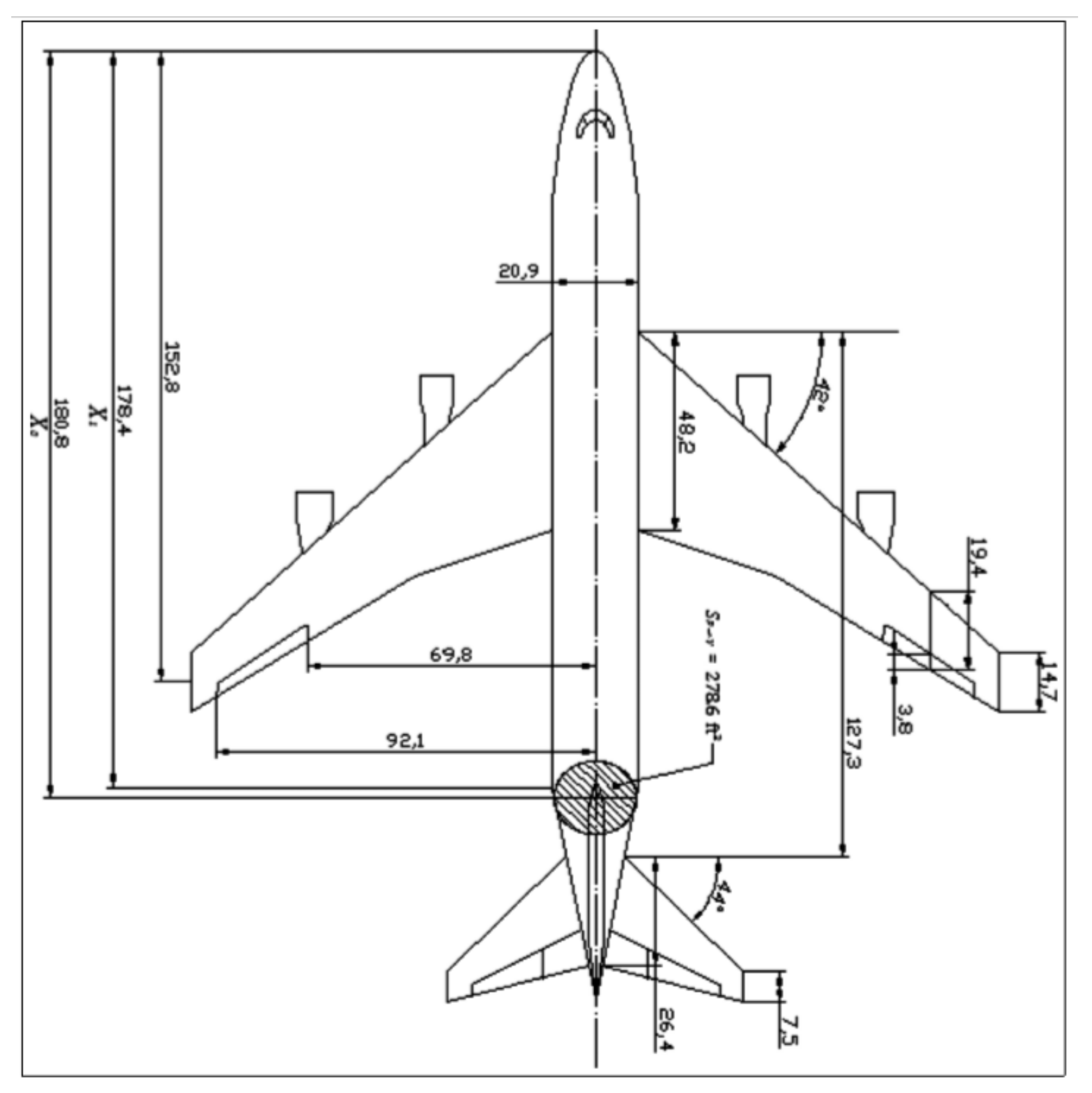
The Boeing 747-200 is a long-range, wide-body, large aircraft designed and developed by Boeing, a commercial airplane company in the USA. It is powered by a high-bypass turbofan engine developed by Pratt and Whitney. Some different variants also have GE-CF6 engines, and original variants have Rolls-Royce RB211 engines. It has a pronounced wing sweep, allowing a cruise Mach number of 0.90. The 747-200B was the basic passenger version of its series with increased fuel capacity and more powerful engines. General specifications of the Boeing 747-200 are given in

Table 1. General specifications of the BOEING 747-200 aircraft [1].

S No.	Specification	Value
1	Maximum takeoff weight	833,000 lbs
2	Total length	231 ft 10 in
3	Cabin width	239.5 in
4	Vertical tail height	63 ft 5 in
5	Fuel capacity	53,985 US gal
6	Thrust	54,750 lbf
7	Range	6560 nm
8	Take off	10,900 ft
9	Type of engine	JT9D-7

.

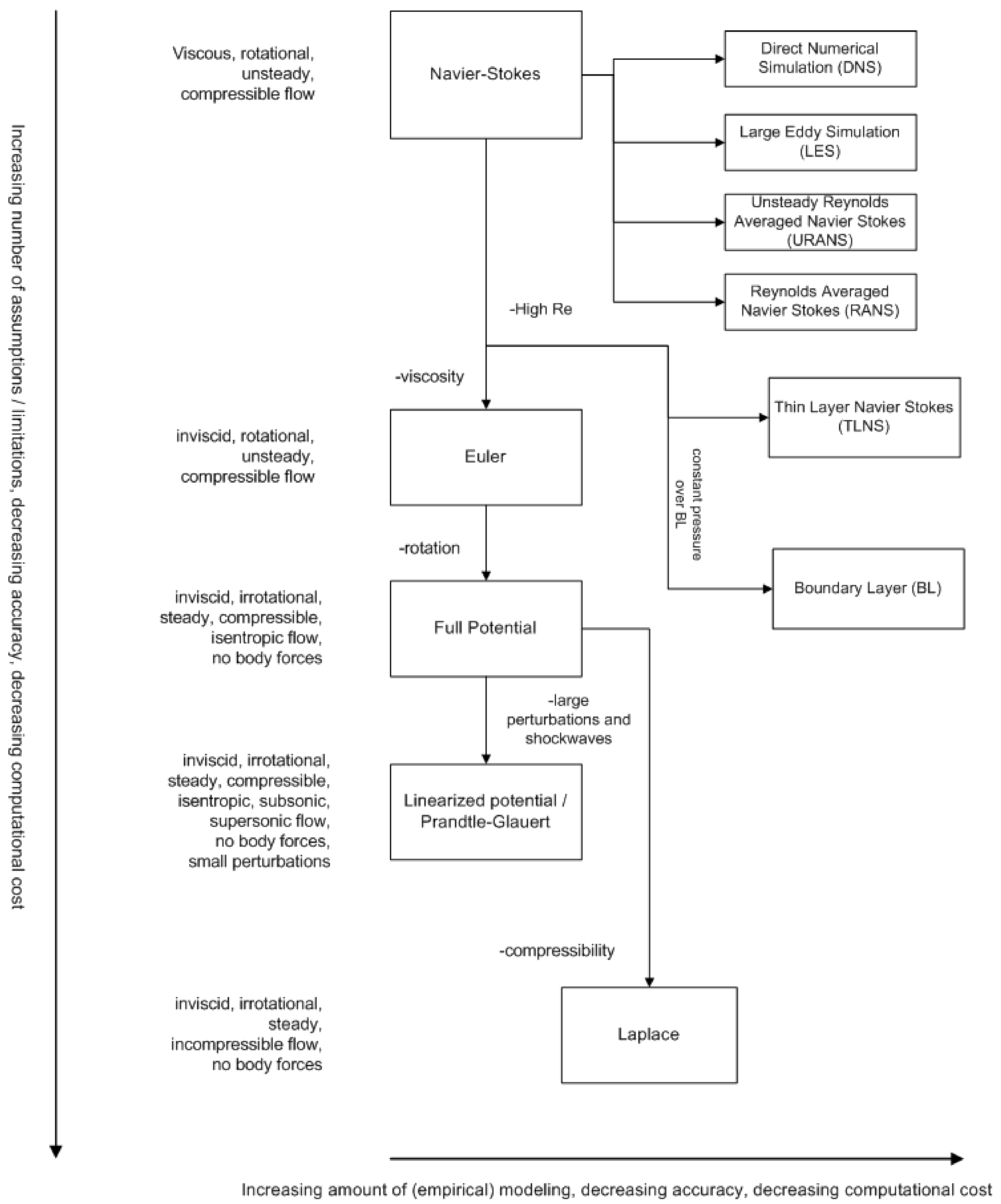
Flow field characteristics can be obtained by applying various aerodynamic flow models. Navier–Stokes (NS) equations are the most accurate flow models that describe viscous, rotational, and compressible flows. These are based on the Eulerian approach and primarily describe the momentum equation. The mass and energy equations are defined using additional relations to solve NS equations [2].

Based on the accuracy and vast applications, NS equations are used in different forms, such as direct numerical solution (DNS), large eddy simulation (LES), unsteady Reynolds-averaged Navier–Stokes (URANS), Reynolds-averaged Navier–Stokes (RANS), thin-layer Navier–Stokes (TLNS), and turbulence modeling (TM) [3]. Boundary-layer equations are based on the concept that at large Reynolds numbers, the viscous effects are limited to a thin region of flow adjacent to the body surface. BL equations are found by dropping the viscous diffusion terms from Navier–Stokes equations because they have little contribution to the solution. The pressure is assumed to be constant along the length in BL models [4]. Euler equations are the conservation laws assuming inviscid flow. The continuity equations do not change; however, energy relations may vary according to the flow characteristics. The assumption of inviscid flow does not limit the applicability of these equations. Moreover, outside the boundary layer, this assumption is also feasible for the flow properties. Modeling flow can be further simplified if the flow is assumed to be irrotational (zero vorticity) [5]. The full potential model combines all the conservation laws (continuity, momentum, and energy equations) [6]. Linearized potential equations are developed by decomposing the velocity into an unperturbed component and a perturbed component, which helps one to solve the non-linearity. Prandtl–Gluert’s relation applies to the flows outside the transonic and hypersonic regimes [7]. For an incompressible flow, the Laplace equation in full potential form is reduced to partial differential equations. The Laplace equation has linearized behavior and has an exact solution. The discretization form of this equation is not required, and hence numerical errors do not exist [8]. Empirical methods do not model the flow; however, these can be used for the estimation of aerodynamic performance [9]. Estimations of lift, drag, and aerodynamic efficiency can be performed by using empirical methods. These methods are further used for stability and control derivatives of the complete aircraft, for instance, in US DATCOM (United States Data Compendium). The evolution of various aerodynamic flow models is described in the flow chart shown in Figure 1.

Aerodynamic coefficients can be estimated using experimental and computational techniques. There are various computational techniques available, e.g., DATCOM, XFLR, TORNADO, AVL, PANAIR, and ANSYS. Each technique has its limitations that restrict its areas of application. TORNADO is a program based on potential flow theory that incorporates the vortex lattice method as its background theory. The wake from lifting surfaces creates vortices and TORNADO captures these effects through horse-shoe or horse-sling arrangements. This program determines the first-order derivatives using a central-difference calculation with the help of a pre-selected state and a disturbed state. The results obtained are accurate only for small rotations or small angles of attack. Moreover, compressibility effects are also not catered to in TORNADO; hence, high Mach number situations cannot be handled accurately [12].

Athena Vortex Lattice (AVL) was developed for the MIT Athena TODOR aero software collection. AVL also solves potential flow through the vortex lattice method. It assumes quasi-steady flow and the compressibility effects are provided through the Prandtl–Gluert model. This program was designed for thin airfoils, small angles of attack, and sideslip. Since slender body analysis is not accurate, it is often suggested to leave fuselage out of the analysis in AVL [13]. Panel Aerodynamics (PANAIR) is a program that uses a higher-order panel method to predict boundary value problems using Prandtl–Gluert relations. It provides a higher-order modeling capability in subsonic and supersonic regions. PANAIR revolutionized the supersonic surface modeling in contrast to average surface meshes. The higher-order panel method yields accurate velocity distributions. PANAIR cannot predict flow dominated by viscous and transonic flow effects. Automatic wake determination through PANAIR is also not accurate. Moreover, for configurations with different total pressures, this program cannot accurately predict the flow characteristics [14]. FLUENT and CFX are two modules of ANSYS. FLUENT employs a cell-centered method and CFX works on a vertex-centered approach. This software can handle different types of meshing operations. such as polyhedral and cut cell meshing (in the case of FLUENT) and tetra and hexa mesh topologies (in the case of CFX). ANSYS is an excellent tool to determine stability and control characteristics, but it takes a long time and has a complex mesh generation process. For industry, it is an ideal tool, since its accuracy and precision is comparable to wind tunnel testing.

Aerodynamic Model Builder (AMB) is a module dedicated to stability and control of the aircraft. It is used to estimate the aerodynamic forces and moments [15,16]. Unlike DATCOM, aerodynamic analysis can be performed in TORNADO software. Moreover, compressible and non-viscous flows can be solved using EDGE (CFD solver) for an irregularly structured tetrahedral mesh produced by the mesh generators SUMO and Tetgen [15]. The feasibility of hypersonic flight is highly dependent on the controller’s design. Due to extreme flow conditions, it is a challenge to develop a design for a large flight envelope and strong interactions between propulsion and structural systems [17,18]. However, the control-oriented model, truth model, wing-cone model, curve-fitted model, and re-entry motion are few techniques with which to take up this challenge [17]. The aerodynamic stall is an important phenomenon while determining the stability and control characteristics [19,20]. Beyond this point, non-linearities and instabilities appear in the flow, and analysis models must be accurate to comment on the complicated flow field. Bifurcation analysis is a tool that discusses the effect of unknown pitch damping dynamics when the aircraft is under a deep-stall transition [21]. Another approach to study the instability effects in time-domain methods is the recursive least squares. The technique uses a recursive formulation to account for residuals, encountered during estimation of aircraft parameters [22,23]. The flow phenomenon over the control surfaces or wing may undergo large variations; therefore, precise simulations are required to obtain accurate results [20,24]. In order to predict the responses for unsteady and nonlinear flight envelopes in high maneuvering operations, extensions to aerodynamic models need to be incorporated [25]. Due to extreme flight conditions, civil or military aircraft may cross normal operating limits. Therefore, prevention or recovery methods are also required to be incorporated in the aerodynamic model [26]. The development of extensive aerodynamic modeling techniques can fulfill these requirements [19]. Information about identification of model can also be obtained from dynamic test methods [27]. The modeling of rotorcraft aerodynamic interference has proven to be a challenging problem due to the complex flow-field interactions between the rotors and other aircraft subsystems. An effective and efficient aerodynamic simulation tool was proposed by combining a Lagrangian solver [21,28]. Data obtained from a quick accesses recorder (QAR) is another efficient way to determine the effects of extreme weather conditions [22,29].

Bryan introduced the theory of aerodynamic derivatives in 1911, and it has remained unchanged as the standard pattern for the interpretation of the aerodynamic loads in equations of motion (EOMs). Aerodynamic forces and moments are assumed to be the functions of control angles, disturbance velocity, and rates of control angles. At low angles of attack (AoA) and in slow-moving airplanes, aerodynamic loads can be easily modeled by using static derivatives. However, at high AoA, dynamic derivatives can greatly affect the stability characteristics [30]. The variation in the stability derivative can be taken into account by adding the non-linear terms along with extensions in the range of flight conditions [31]. Grauer and Morelli [32] developed a procedure to determine the single generic global aerodynamic model structure that could be applicable to various aircraft. The analysis was carried out by applying multivariate-orthogonal-function modeling on wind-tunnel aerodynamic databases of different aircraft over a wide range of angles, rates, and deflections of control surfaces.Drela et al. [33] investigated the aerodynamic benefit from ingestion of boundary layer of a transport aircraft. The power balance method was developed based upon the mechanical power required and streamwise forces acting on the aircraft. The results showed an increase in efficiency of up to 9% at low cruise power conditions. Grauer and Morelli [34] developed a generic nonlinear aerodynamic model based upon multivariate orthogonal function. The model accurately predicted the global and local dynamic behavior and trim solutions over a range of large amplitude excitations. Triet et al. [35] and Nguyen et al. [36] performed aerodynamic analysis of an aircraft wing using computational fluid dynamics. The variation of velocity and pressure distribution on the wing was captured by using ANSYS Fluent package. The coefficients of lift and drag were estimated based upon data obtained at different boundary conditions. Vecchia and Nicolosi [37] provided the guidelines in the design and optimization of transport aircraft. MATLAB algorithm was developed to determine the aerodynamic coefficients. The panel code solver was used to optimize the geometrical shapes. The procedure helped to import and modify geometries by interpolation of curves and surfaces.Nicolosi et al. [38] presented a method to determine the aerodynamic performance of aircraft fuselage. During the study, the contribution of the fuselage to overall stability and its interactions with the wings and tail were investigated. Numerical simulations were carried out based upon CFD techniques and aerodynamic coefficients were estimated. Ammar et al. [15] performed the stability analysis of a blended-wing-body aircraft. The static and dynamic stability and flying quality analysis was carried out in a flight envelope by applying aircraft synthesis and integrated optimization methods. The flight envelope was created and the TORNADO program was used to estimate the aerodynamic coefficients of aircraft. Rizzi [39] presented an overview of the simulated stability and control system of an aircraft. Flying and handling qualities were determined using integrated optimization techniques. Lu [40] investigated the dynamic stability and control characteristics of a tilt-rotor aircraft using mathematical nonlinear flight dynamics techniques. The damping coefficients in longitudinal and lateral modes were estimated and their effects on overall stability characteristics were analyzed.

The geometric parameters along with flight conditions are the basic and most important requirements for modeling the aircraft in any software. The data of a Boeing 747-200 are readily available in online sources to be used as the foundations of modeling and analysis of the aircraft. The geometric parameters along with control surface clearances were acquired from established literature and reliable online sources [41]. Based upon theoretical knowledge such as the vortex latex method (VLM), source code was generated in both computer programs. For modeling of aircraft to acquire stability and control derivatives, design flight conditions were used. Analytical results available in the literature for low-cruise-flight conditions were selected as a benchmark. Figure 2 shows the flow chart of the methodology adopted during the project. The parameters in both software applications were derived from basic equations of motion (Equations (1)–(6)) for an aircraft (six degrees of freedom system) readily available in the literature [1,42].

Force equations:

$$F_x=M(\frac{du}{dt}+qw-rv)$$

(1)

$$F_y=M(\frac{dv}{dt}+ru-pw)$$

(2)

$$F_z=M(\frac{dw}{dt}+pv-qu)$$

(3)

Moment equations:

$$l=I_x\frac{dp}{dt}-I_{xz}\frac{dr}{dt}+qr(I_z-I_y)-I_{xz}pq$$

(4)

$$m=I_y\frac{dq}{dt}+I_{xz}(p^2-r^2)+pr(I_x-I_z)$$

(5)

$$n=I_z\frac{dr}{dt}-I_{xz}\frac{dp}{dt}+pq(I_y-I_x)+I_{xz}qr$$

(6)

where l, m, and n represent the rolling, pitching, and yawing moments. $F_x$, $F_y$, and $F_z$ represent the resultant forces in longitudinal, lateral, and vertical axes, respectively. The symbols M and t represent the mass of the body and the time domain, respectively. The symbols u, v, and w represent the axial, side, and normal velocity components, respectively. The symbols p, q, and r represent the roll, pitch, and yaw rates, respectively. $I_x$, $I_y$, and $I_z$ represent the moment of inertia components in x, y, and z-axes. $I_{yz}$, $I_{zx}$, and $I_{xy}$ represent the products of inertia in roll, pitch, and yaw axes.

The equations of motion are derived for a particular axis system specific to the aircraft. Equations for aerodynamic, gravitational, and propulsive are derived using Newton’s equations of motion while applying Euler angle corrections to make the equations consistent in one frame of reference. Small-angle approximation and steady flight conditions are used to linearize the equations with the assumption that small perturbations occur in the motion of an aircraft during steady flight. This assumption holds good for the theoretical determination of stability for the small-amplitude motion of aircraft. Once employed, forces/moments in x, y, and z-directions are computed and observation is the coupling of lateral and directional motion. The stability and control of an aircraft can be troublesome if things are discussed in theoretical form but a representation using stability and control coefficients makes life easier. After the development of complete linearized equations of motion, Taylor’s series expansion is used to determine the relations of the rates of change of stability parameters. The expressions of stability/control coefficients and derivatives are used in software solutions to run the simulations of modeled aircraft. The results are obtained using visual tools along with insights into the aerodynamic behavior of aircraft during motion.

In the present research, stability parameters for wide-body aircraft have been estimated using computational techniques. The comparison of statistical software (DATCOM) with a computational technique (XFLR) for a wide-body Boeing 747-200 is also presented. Although these software programs have been tested and evaluated multiple times, a one-to-one comparison for a Boeing 747-200 is the first of its kind. Results obtained from US DATCOM and XFLR software were compared for any differences and the they were also validated with analytical correlations presented in the literature. The material covered in the different sections is as follows.

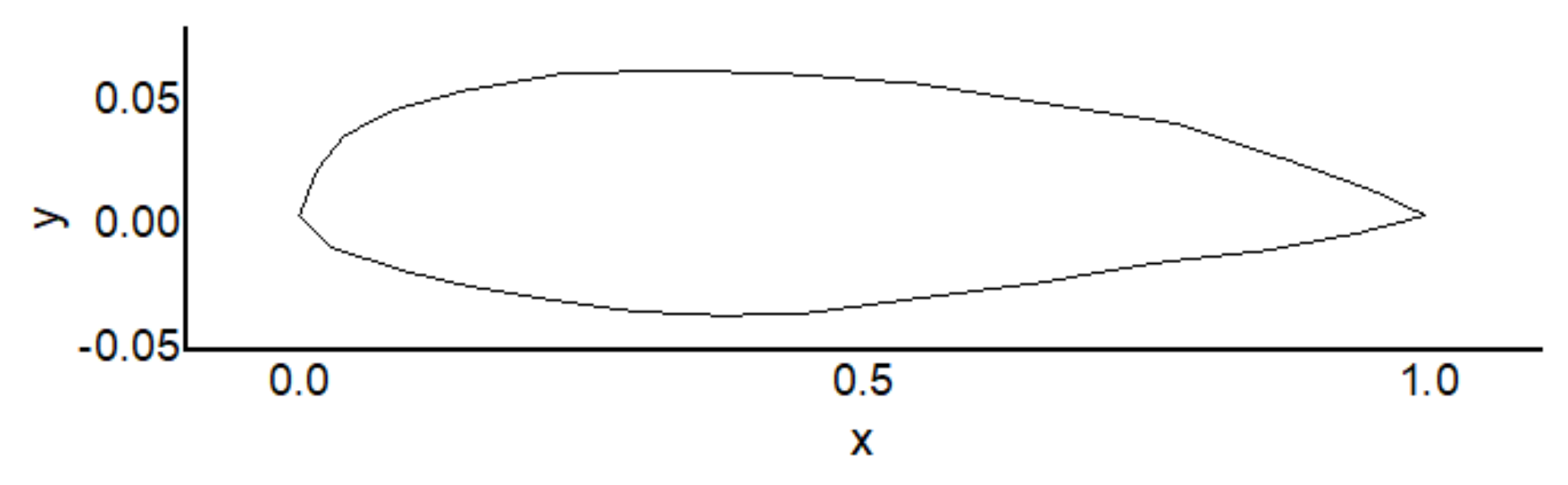
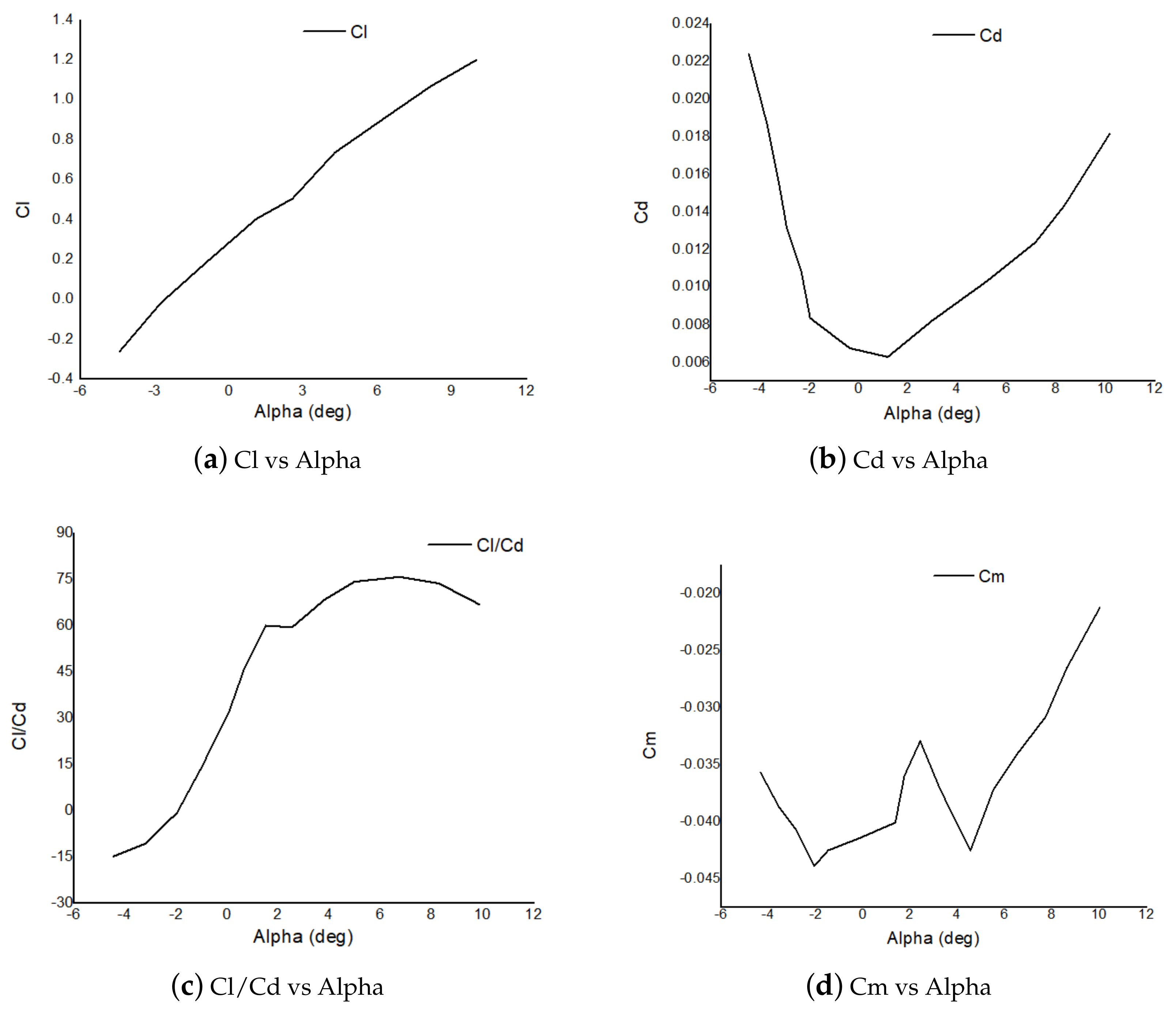
In the second section, a brief overview of the US DATCOM algorithm, its applications, and its working principle to determine the stability and control coefficients have been discussed. Aerodynamic coefficients of a wide-body airplane have been estimated at given flight conditions. The variations of lift, drag, and moment coefficients have been obtained at various angle of attack. Moreover, longitudinal and lateral aerodynamic coefficients have also be acquired at different angles of attack and control surface deflections. In the third section, the XFLR algorithm to determine the stability and control analyses of an aircraft has been elaborated. The various applications and limitations of XFLR in aircraft design and analysis have also been discussed. In order to estimate the aerodynamic coefficients of Boeing 747-200 aircraft, the elements of the design process, including direct foil analysis, and wing and body design and analysis have been elaborated. The results of lift, drag, and moment coefficients have been acquired at different angles of attack and they have been plotted. Moreover, to check the stability conditions, eigenvalues for longitudinal stability (short period and Phugoid) and lateral stability (spiral, roll, and Dutch roll) modes have also been evaluated. In the fourth section, results obtained from both the commercial packages are presented in terms of dimensionless aerodynamic coefficients. Results obtained at low-cruise-flight conditions have been compared with the analytical results available in the literature. The comparative analysis shows that results obtained from computational techniques are quite close to each other and to the analytical results. 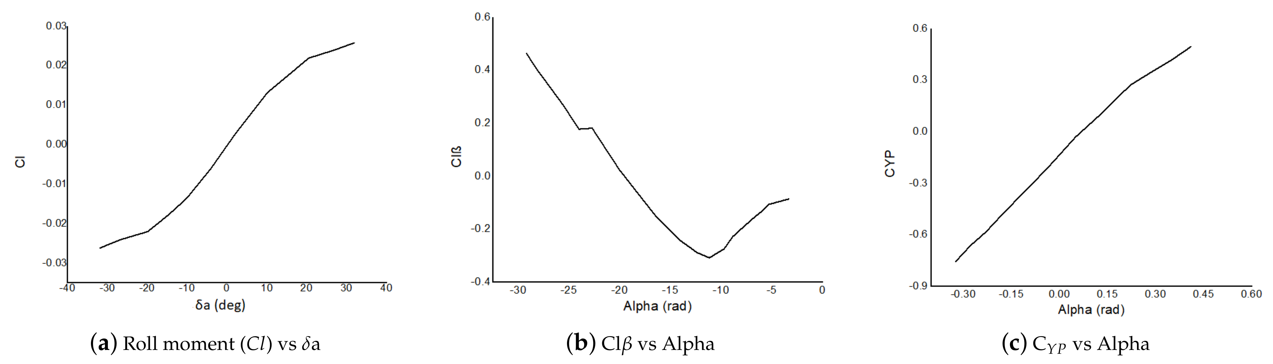The comparison of longitudinal and lateral coefficients obtained from both pieces of software with the results available in the literature is summarized in Appendix A. In the fifth section, analysis and discussion of the results obtained from both pieces of software have been given. Aerodynamic coefficients having a great influence on the accuracy of the results for the validation of the codes are also presented. Moreover, a graphical representation of aerodynamic coefficients at different angles of attack have also been added. In the sixth section, the conclusions have been drawn based on a comparison of results and computational analysis. The analysis provides meaningful results for the estimation of longitudinal stability and control derivatives from the knowledge of aircraft geometrical parameters and given flight conditions. In order to improve the source code by exploring some advanced features, a few recommendations have also been added in that section.

2. US DATCOM

DATCOM is a computer algorithm that is used to estimate the aerodynamic properties, i.e., stability and control coefficients of fixed-wing aircraft either by extrapolation or interpolation of information available in a database [43]. The computer program was modified into commercial software that has been extensively used in academia as one of the reliable tools for the stability and control of an aircraft. The software now is in the public domain and has been replaced in the aerospace industry by newer computational analysis options [44,45]. It is a combination of theoretical and experimental procedures that are required to analyze aerodynamic stability and control parameters. DATCOM can be used for the autonomous design of the flight control system for a fixed/blended wing aircraft [46]. Aerodynamic parameters are generally obtained from wind tunnel testing, computational fluid dynamics, or flight tests; however, dimensionless aerodynamic stability (static/dynamic) derivatives can be directly estimated using DATCOM [47]. The inputs required in DATCOM are only physical dimensions and flight conditions, but the output can be varied according to the requirements. Not only can the coefficients of the entire aircraft be obtained, but individual surfaces or a combination can also be produced as an output. Additional output configurations include wing, horizontal tail, wing–tail, and wing–fuselage–horizontal tail configurations. In DATCOM, forward lift surfaces are always treated as wing and the aft lift surface is considered as a tail [48]. The analysis gives meaningful results for the estimation of a complete set of longitudinal stability and control coefficients for lifting, stability, and control surfaces. Aircraft model simulation can also be obtained to visually check the various surfaces. Figure 3 shows the Boeing 737 model obtained from DATCOM based upon geometric parameters. The output can further be utilized to evaluate the flight dynamics characteristics. Aircraft control surface deflections and aerodynamic data at various Mach number regimes can also be computed [49].

The characteristics based on body aerodynamics and subsonic longitudinal data can be obtained at different Mach numbers for rotational and cambered bodies having arbitrary cross-sectional areas [50]. Moreover, the trim output can also be computed by the manipulation of stability and control characteristics. The trim mode includes a horizontal tail or wing coupled with a trim control mechanism and longitudinal aerodynamic characteristics, and deflection angles required to trim are obtained as outputs. Some special control procedures, i.e., hypersonic flap methods related to controllability and stability for high-speed operating devices, are also incorporated in DATCOM. The initial sizing procedure of 2D transverse jet controls for an aft-end located nozzle operating at a high Mach number can be obtained from this technique. Moreover, the interaction of the local flow field and transverse jet can also be evaluated. The output from DATCOM can be imported into MATLAB through the MathWorks Aerospace Toolbox where static and dynamic stability and control derivatives can be stored in arrays that can be further used in the Simulink block for stability analysis.

2.1. Aerodynamic Coefficients Estimation Using US DATCOM

DATCOM treats various high lift devices, including plain, single/double slotted jet flaps; leading-edge flaps; and control devices, such as spoilers and typical wing–body–tail configuration with controlled effectiveness. The software application is well-designed for the conventional aircraft configurations [51]. The characteristics including lateral, longitudinal, and directional stability obtained from DATCOM are in the stability axis system. For specific configurations and Mach number regimes, coefficients, e.g., Cl$\beta$, Cm$\alpha$, Cn$\beta$, CL$\alpha$, CL, Cm, and CD, can be obtained from the DATCOM output file. Additionally, parameters such as lift, roll, moment, normal dynamic derivatives, side-force for the angle of attack, and angular rates can also be computed [48]. Flight conditions are defined in DATCOM based on Reynolds number and Mach number data. This condition can be satisfied by defining velocity, altitude, temperature, and pressure along with the requisite Reynolds number and Mach number. In the present study, aerodynamic coefficients of the Boeing 747-200 airplane at low-cruise-flight conditions (M = 0.5, Alt = 20,000 ft, and $\alpha$ = 6.8 deg) were estimated.

2.2. Geometric Parameters

Geometric parameters required for analysis (estimation of aerodynamic coefficients) were obtained from the established literature and reliable online sources. Some of those parameters are given in

Table 2. Geometric parameters of BOEING 747-200 aircraft [52].

S No.	Geometric Parameter	Symbol	Value
1	Reference area	S	5500 ft${}^2$
2	MAC	$\overline{C}$	27.3 ft
3	Wingspan	b	196 ft
4	Mach No (cruise)	M	0.9
5	True airspeed	V	871 ft/s
6	Dynamic pressure	P	222.8 Psi
7	CoG location	Xcg/$\overline{C}$	0.25
8	Angle of attack (cruise)	$\alpha$	2.4 deg
9	Weight	W	636,636 lbs
10	Moment of inertia	Ixx	1.82 × 10${}^7$ slug-ft${}^2$
11	Moment of inertia	Iyy	3.31 × 10${}^7$ slug-ft${}^2$
12	Moment of inertia	Izz	4.97 × 10${}^7$ slug-ft${}^2$
13	Inertia moment product	Ixz	9.7 × 10${}^5$ slug-ft${}^2$
14	Fuselage length	L	225.17 ft
15	Wing sweep angle	∧	37.5 deg
16	Aspect Ratio	AR	7

.

The scaled-down model drawings of the Boeing 747-200 airplane with dimensional parameters and horizontal/vertical clearances obtained are shown in Figure 4. Based upon geometric parameters and horizontal/vertical clearances, source code was generated in DATCOM by applying VLM theory.

2.3. US DATCOM Results

After the generation of source code, stability/control analysis was carried out, and results from US DATCOM at low-cruise-flight conditions with variations of the angle of attack and control deflection were obtained. The variation of different stability/control coefficients in both longitudinal and lateral modes can be seen with the angle of attack and control deflection in the plots shown below.

2.3.1. Evaluation of Lift, Drag, and Moment Coefficients

Variation of basic aerodynamic coefficients of lift, drag, and moment with the angle of attack is shown in Figure 5. The plots show similar trends with stable conventional aircraft. Figure 5a shows a variation of lift coefficient with an increasing angle of attack. The values of CL0, CL$\alpha$, and CLmax came out to be 0.12, 4.76, and 1.78, respectively. For the range of angle of attack ($-0.4$ to 0.5 rad), the stall lift coefficient can also be seen in the plot. A variation of drag coefficient for a range of angles of attack is plotted in Figure 5b, which gives a similar trend as the original aircraft, thereby verifying the results of DATCOM in the determination of the stability of the 747-200. The value of CD0 is 0.020; it is in agreement with the performance data of Boeing aircraft found in the literature. The zero-drag coefficient is an important parameter in the design phase of the aircraft.

The value of the drag coefficient increases with increases in the angle of attack, leading to an increase in the lift. For a longitudinally stable aircraft, the value of the y-intercept of the Cm$\alpha$ curve should be positive and the moment coefficient against a changing angle of attack must have a negative slope. The plot depicts the expected result, establishing that the selected aircraft results satisfy this condition of stability. The result shows that the aircraft has an inherent ability to generate a longitudinal counter moment as soon as it experiences a disturbance while airborne. The sensitivities of the air vehicle towards a disturbance and the associated response (as shown in the Figure 5c) are basic stability measuring criteria.

2.3.2. Longitudinal Aerodynamic Coefficients

Results for longitudinal aerodynamic coefficients, i.e., CL$\alpha$dot, Cm$\alpha$dot, CD$\delta$e, and CD$\delta$f etc., with the variations in the angle of attack and control surface deflections, were obtained and plotted in Figure 5 and Figure 6.

Not only are simple stability coefficients plotted in DATCOM, but it also gives plots for the angle of attack rate. Figure 5d gives an increasing trend of lift coefficient at the start that subsequently decreases due to the angle of attack rate, which is in concurrence with the original aircraft behavior in flight. Since the Boeing 747-200 has an aft–tail configuration, the lift coefficient due to pitch rate is a positive value throughout the flight. The variation of the moment coefficient with the rate of change of angle of attack as shown in Figure 5e suggests a nonlinear trend. It is one of the pitch damping derivatives that shows an unsteady increase in the moment coefficient as soon as the angle of attack rate changes. The plot shows an initial decrease in moment coefficient at a negative angle of attack rate. Subsequently, a positive slope is obtained for the range of angle of attack rate, thereby increasing the pitching vibration in the aircraft structure.

Elevator deflection affects drag, and a plot of drag coefficient is drawn in Figure 6a to observe the behavior of aircraft when subjected to the deflected elevator over a range of deflection angles. Another trend for drag coefficient is plotted in Figure 6b to study the effect of flap deflection on the drag, which can be explained in terms of pressure changes that ultimately affect the drag force.

2.3.3. Lateral Aerodynamic Coefficients

Results of lateral aerodynamic coefficients with a variation of the angle of attack and control surface deflections were obtained and plotted in Figure 7. According to the theory, the roll moment coefficient for a stable aircraft must have a positive slope. The plot from DATCOM shows a positively increasing slope, thereby verifying that results obtained from software agree with conventional aircraft behavior. The rolling moment due to changing side-slip has a negative slope and the plot satisfies the stability condition for lateral motion.

The plot of side force with a change in roll rate shows an increase in force as the roll rate increases. This plot is in concurrence with the theory and proves that lateral and directional motions of an aircraft are coupled. The longitudinal stability aerodynamic coefficient results obtained at low-cruise-flight conditions are shown in

Table A1. Comparison of longitudinal stability aerodynamic coefficient results.

S No.	Parameter	Analytical [62]	DATCOM	XFLR	Abs Err DATCOM	Abs Err XFLR
1	CL	0.68	0.679	0.623	0.001	0.057
2	CD	0.0393	0.0371	0.036	0.0022	0.003
3	$CL\alpha$	4.67	4.76	3.62	0.09	1.05
4	$CD\alpha$	0.366	0.329	0.315	0.037	0.051
5	$Cm\alpha$	−1.146	−3.22	−3.83	2.074	2.684
6	$Cl\alpha$dot	6.53	1.693	-	4.837	-
7	$Cm\alpha$dot	−3.35	−8.33	-	4.98	-
8	Clq	5.13	8.72	6.39	3.59	1.26
9	Cmq	−20.7	−28.8	−23.55	8.1	2.85
10	CLM	−0.0875	−0.102	−0.042	0.0145	0.0457
11	CDM	0.0	0.0	0.0	0.0	0.0
12	CmM	0.121	0.153	0.213	0.032	0.092
13	$Cl\delta$e	0.356	0.42	0.52	0.064	0.164
14	$Cm\delta$e	−1.43	−1.37	−2.09	0.06	0.66

of Appendix A. The results obtained from US DATCOM are very close to the analytical results; however, the reason for the large absolute error in some of the parameters, i.e., Cl$\alpha$dot, Cm$\alpha$dot, and Clq, is that DATCOM is a traditional aircraft sizing technique, and it employs methods resulting from an empirical source to approximate the stability parameters. Results obtained at low values of angle of the attack indicate a close correlation. Similarly, the lateral stability aerodynamic coefficients’ results obtained at low-cruise-flight conditions are shown in

Table A2. Comparison of lateral stability aerodynamic coefficient results.

S No.	Parameter	Analytical [62]	DATCOM	XFLR	Abs Err DATCOM	Abs Err XFLR
1	$Cy\beta$	−0.9	−0.92	−0.893	0.02	0.007
2	$Cl\beta$	−0.193	−0.319	−0.18	0.126	0.013
3	$Cn\beta$	0.147	0.32	0.21	0.173	0.063
4	Clp	−0.323	−0.328	−0.41	0.005	0.087
5	Cnp	−0.0687	−0.16	0.057	0.0913	0.1257
6	Clr	0.212	0.231	0.227	0.019	0.015
7	Cnr	−0.278	−0.61	−0.33	0.332	0.052
8	$Cl\delta$a	0.0129	0.0201	0.0135	0.0072	0.0006
9	$Cn\delta$a	0.0015	0.004	0.0026	0.0025	0.0011
10	$Cy\delta$r	0.1448	-	0.132	-	0.0128
11	$Cl\delta$r	0.0039	-	0.0027	-	0.0012
12	$Cn\delta$r	−0.1081	-	−0.107	-	0.0005

of Appendix A. Results obtained for directional and lateral coefficients are also quite close to the analytical results. Rudder control derivatives could not be estimated because there is no option for giving rudder input in DATCOM. The error can be further reduced by using more accurate geometric measurements of the airplane and by referring to the available upgraded version of the software.

3. XFLR

The stability and control analysis of an aircraft has been an exclusive subject in the field of aeronautics. Software solutions such as XFLR have been designed to study stability and control dynamics. This evolution has not only aided in the dynamic modeling of the aircraft but also contributed to the study of aerodynamics. XFLR is a piece of stability analysis software in which there is an easy means of drawing up the aircraft according to the physical measurements and performing aerodynamic analysis to obtain the necessary aerodynamic data for the evaluation of stability derivatives. It is a tool used to analyze a wing, airfoil, or complete airplane with various Reynolds number operations [53]. It is also compatible with Windows as well as LINUX and is easily downloadable. Originally, XFoil was written in FORTRAN, but now the code has been translated into C/C++ for XFLR. The latest version of the software introduces the stability analysis of the planes. It also has inverse and direct analysis capabilities for XFoil [45]. XFLR uses forward differentiation for the determination of the stability and control derivatives. Hence, the derivatives are computed through Taylor’s series approximations in this software solution.

3.1. XFLR Analysis Technique

The preliminary task to perform for analysis in XFLR is the modeling of a wing, aircraft, or any lifting surface. The 3D panel method, the vortex lattice method (VLM), and lifting line theory (LLT) are employed to analyze wing/airfoil design and perform various other analyses. Each method has its own salient features for different applications; i.e., lift curve slope accounting for the viscous effects can be precisely estimated using the LLT approach. However, there are some limitations of these methods as well; i.e., the panel method does not improve the accuracy of the results notably. It has been observed that the obtained values of aerodynamic forces/moments using this software approach are very close to the experimental results. XFLR comprises of XFoil program for foil analysis and three-dimensional analysis methods for the planes that include: (i) stability analysis of the planes, (ii) a two vortex-lattice method and a 3D panel method for the analysis of the aerodynamic performance of wings/plane operating at low Reynolds numbers, and (iii) a non-linear lifting line method for a standalone wing. Radio-controlled (RC) aircraft can also be designed by using XFLR software [54]. Another application of XFLR software is to analyze the two-dimensional viscous results obtained from the XFoil subsonic airfoil development system and the time-independent incompressible flow solution obtained from the Laplace equation. Even for aircraft design, the foremost step is to analyze the associated airfoils before exclusively proceeding with the aircraft design [45]. In order to analyze the wing/tail airfoil, coordinates are imported in XFLR, and geometry is generated. Figure 8 shows the airfoil geometry developed and analyzed in XFLR.

The variations of moment, lift, and drag coefficients are obtained during aerodynamic analysis. Moreover, airfoil analysis, as well as pressure distribution, can also be obtained to study the performance characteristics. The pressure distribution depicted by the graphical result also provides an insight into the separation region. In XFLR, the entire aircraft can be modeled with the liberty of creating different auxiliary lifting surfaces. This software is widely used in aircraft design and the computed data agrees with the XFoil software. Experiments have shown that XFLR produces reliable results based on the vortex lattice method, as these results were verified by wind tunnel tests. The correlation between XFLR and ANSYS software can be established to obtain more realistic data and to verify the setup used. Aircraft dynamics can also be simulated using control/stability derivatives with the help of XFLR modeling; i.e., elevator deflection at specific trim conditions can be simulated by modeling aircraft with known dimensions. The stability augmentation system of the flying wing can be used to determine the feedback control obtained from proportional derivatives to reduce pitch instability [44]. Another application is to simulate the sideslip and angle of attack with the help of XFLR modules. In XFLR, the order of sideslip and angle of attack applications has its significance. (i) The model analysis is carried out by conventional panel or vortex lattice technique, (ii) sideslip is designed by model rotation about the z-axis, and (iii) this method is preferred, as the implementation of this technique is comparatively simple. By convention, sideslip rotation is applied after the angle of attack and the final position may be slightly different as compared to the experimental results at high sideslip or angle of attack values. The rolling/yawing moments and coefficients of lateral forces can also be determined from the non-viscous portion of the panel or vortex lattice method. Theoretically, the results are closed at all speeds; however, a difference may be observed during experimentation that leads to the effect of viscosity on the distribution of pressure forces. After the 3D model of the aircraft is obtained, stability derivatives and aerodynamic coefficients can be estimated with the help of different algorithms using the XFLR program. XFLR software can also be applied to compare the performance parameters of various airfoils [55]. It has been observed that the three-dimensional panel technique can be used to regulate the aerodynamic loads for some airfoils at different angles of attack. During the analyses of the designed aircraft model with or without the body, using any of the three methods, i.e., LLT, 3D panels, or VLM methods, it has been established that all three methods can correctly predict the lift coefficient at zero moment value and the moment coefficient at zero lift with some exceptions [56,57]. Moreover, a tolerable trend of Cm$\alpha$ can also be obtained by using LLT or VLM methods. Modeling can generate numerical noise because of flow-field interference between the body and the wing [58]. Stability analyses can also be carried out in XFLR software. There are three major elements of stability analyses—i.e., (i) the open-loop dynamic response contains hands-off control and can get the perturbation, i.e., the wind gust from the airplane’s response; (ii) airplane’s response in natural modes is captured at natural frequencies; (iii) the response obtained from forced dynamic input is directed to control actuation, i.e., elevator or rudder. One of the requirements of control and stability system analyses is to define the inertial characteristics. Inertia can be roughly approximated using XFLR with the available data of geometry and mass distribution, e.g., fuselage structure; wing mass; and locations/masses of servo-actuator, battery, nose lead, and receiver [59].

3.2. XFLR Methodology

The design process in XFLR starts with airfoil analyses. To design wing and tail surfaces of Boeing 747-200, two airfoils (BACxxx and NACA 0012) were used. The former was imported from the airfoil database available online and NACA airfoils are available in XFLR’s in-built library. When airfoils were successfully imported in direct foil design, the number of panels was adjusted to 120. The number of panels had to be selected to get sufficient data points of leading and trailing edges. The flap deflection is generally set between −10 to 10 degrees. Once settings were done, foil analysis could then be performed. A multithread analyses option studies multiple foil simultaneously. The range of Reynolds number was adjusted to between 100,000 and 500,000. In order to study the aerodynamic characteristics, the airfoil analyses are recommended before creating the aircraft model. Airfoil characteristics are obtained graphically in the form of lift, drag, longitudinal moment, and pressure distribution over the length of airfoil. Once the stability parameters are achieved (Cm$\alpha$ < 0, Cm0 > 0), the complete aircraft design process can then be completed. During the initial design phase, the wing surface is generated and divided into a number of sections. Each section is assigned a chord length, a twist, and dihedral angles according to the design requirements. Once wing design is completed, the remaining surfaces, i.e., fin and elevator (vertical and horizontal tails, respectively), are created by following the same method. In XFLR, to design the fuselage surface, the body option is selected because it is not part of primary aircraft components. Once the surfaces are generated, the masses for each component of the airplane and some additional masses—passenger, avionics, etc.—are added. The mass distribution must be carried out carefully because it affects the moments of inertia and center of gravity. Aircraft analyses are performed in two phases: aerodynamics and stability. XFLR uses VLM, the panel method, and interactive boundary layer methodology for complete wing analyses. The results are obtained in the form of stability and control coefficients. The flow chart showing the detailed methodology of XFLR is shown in Figure 9.

3.3. Direct Foil Design

The airfoil coordinates were imported from the airfoil database. For the Boeing 747 airplane, airfoil BAC463 and BAC474 were used for root and tip, respectively. If one needs a NACA airfoil, XFLR already has in-built data for this series. For the tail, typically a symmetrical airfoil is used. Hence, XFLR’s in-built NACA library is sufficient for tail design. It is recommended to define flap deflection in the initial stages of design so that flapped airfoils can be analyzed with the rest of the airfoils, although they may be used in the aircraft building later in the project. The airfoil coordinates were imported, and geometry was generated. The XFLR view of the airfoil is shown in Figure 10.

3.4. Direct Foil Analysis

In direct foil analysis, before creating the aircraft body, airfoils are analyzed using VLM theory for viscous and inviscid regimes. Aero data and Reynolds numbers are defined by the user [51,60]. The analyses gives lift, drag, and moment coefficients vs. angle of attack. Pressure distribution over the airfoil can also be obtained. Airfoils are usually put under viscous analyses if one wishes to determine realistic curves for the aircraft [61]. An inviscid airfoil cannot be trusted for viscous analyses of the entire aircraft. There are four methods to analyze the airfoil database; out of those, “Type 1” was selected. Aerodynamic analyses of the airfoil were also carried, and the results obtained for the 2D airfoil through multiple parameters are shown in Figure 11.

3.5. Wing and Body Design

After the generation of airfoil geometry and analyzing it, the wing and body design section creates the aircraft components one by one. Wings, an elevator (H-tail), and a fin (V-tail) are default components. The fuselage is added as a separate body. For every component, the required geometric parameters are:

• Length;
• Chord of the airfoil;
• Location;
• Sweep angle;
• Dihedral;
• Airfoil name.

For the fuselage, an additional requirement is to add sections and divisions along the length and specify their locations along all three axes. The design of the entire aircraft is based on the panel method in XFLR because dividing the geometry in the panels facilitates the analyses of the aerodynamic and stability performance of the aircraft. More panels give an improved analyses, although simulation time may increase or XFLR may crash. Make sure to save every step in the file option from the hot bar, since XFLR can crash anytime and will not retain the memory of unsaved projects. After creating the components, set inertia for each component; XFLR, in turn, calculates the center of gravity (CoG) of the aircraft. Additional masses can be mentioned separately—typically, engines, avionics, hydraulics, and landing gear are added as separate masses to get a realistic CoG of the aircraft.

The software may have sufficient accuracy in its mathematical modeling or framing assumptions, but more background information and appropriate knowledge for all test factors need to be applied. A comparison of results obtained from XFLR can be verified and validated for various Reynolds number designs and computational methods. An example would be the AVL software package of computational fluid comparing different parameters calculated by XFLR to flight test data instead of the stability dynamic modes. For example, performance data can be compared to verify and validate software results [46]. To summarize this, it can be stated that XFLR software is helpful in the aircraft control system design process and can be applied in various applications in the field of aviation.

3.6. Analysis

XFLR gives the liberty of aerodynamic and stability analysis according to the user’s choice. It is recommended to run the aerodynamic analysis first to obtain insights into the performance of the aircraft. The analysis techniques are lifting line theory (LLT), the Horseshoe method, and VLM. The choice of viscous or inviscid is also present. Once the aerodynamic analyses are run, a series of graphs are generated to display the aircraft’s performance through CL, CD, and Cm. After aerodynamic analysis, stability analysis is defined and run for already defined flight conditions to generate stability derivatives, and results are obtained in the form of root locus/time response. Both longitudinal and lateral modes are catered for in XFLR with a detailed review of Phugoid, short period, roll, and Dutch-roll modes of flying aircraft. Animations of all the modes are also available within wide ranges of speeds and amplitudes. The derivatives of stability are stored in a text file with the name of log file. This file also covers eigenvalues and eigenvectors of the aircraft at given conditions.

3.7. XFLR Results

In order to obtain the lift, drag, and moment coefficients, aircraft stability analysis was performed in XFLR software. The variations of lift, drag, and moment coefficients with angle of attack are shown in Figure 12. For a range of angle of attack from $-6$ to 17 deg, a linear relationship between lift coefficient and angle of attack is visible (Figure 12a). The choice of a range of angles was deliberate because, in this range, the stability of the aircraft is most prominent. An angle less than $-6$ degrees would give a useless result and an angle more than 17 would be beyond the stall region. The variations of lift and drag coefficient (Figure 12b) obtained from XFLR agree with typical drag polarity drawn for conventional aircraft. For Boeing 747-200, the results are as per design requirements ensuring smooth aerodynamic performance. The graph (Figure 12c) shows a proportional relation between aerodynamic efficiency and angle of attack, indicating the promising aerodynamic performance of the aircraft in the given regime. The result is in concurrence with the theory of stable flight. Figure 12d shows the linear relationship between lift and moment coefficients with negative slope values, such as the variation of moment coefficient, with angle of attack. For a longitudinally stable aircraft, the value of Cm0 should be positive; i.e., the y-intercept of the Cm$\alpha$ curve should be positive and the moment coefficient against a changing angle of attack must have a negative slope. The plot depicts the expected result establishing that the selected aircraft results satisfy this condition of static stability. The longitudinal stability aerodynamic coefficients results obtained at low-cruise-flight conditions are shown in Table A1 of Appendix A. CL$\alpha$dot and Cm$\alpha$dot could not be estimated by XFLR due to software limitations. The results from XFLR are close to the analytical results; however, small errors occurred due to approximations used in the software. Moreover, due to panel creation, some errors may also occur because the wing panel’s wake interacts with the fin and elevator to generate unwanted numerical interactions. Similarly, the lateral stability aerodynamic coefficients results obtained at low-cruise-flight conditions are shown in Table A2 of Appendix A. The obtained results are close to the DATCOM results and analytical results, despite small absolute differences in some of the parameters. The results may vary because XFLR’s wake modeling is insufficient to cater for flow behavior experienced by aircraft in real flight. Moreover, the effect of the fuselage is not added in the XFLR analysis of the entire aircraft.

Eigenvalues are a special set of scalars associated with a linear system of equations also known as characteristic roots, characteristic values, proper values, or latent roots. These are used to determine the stability and the rate of decay/growth of the system. For the present case, eigenvalues for longitudinal (short period and Phugoid) and lateral modes (spiral, roll, and Dutch roll mode) were also estimated, as shown in

Table 3. Eigenvalues obtained from XFLR for the Boeing 747’s dynamic stability analysis.

S No.	Eigen Value	Mode	Stability
1	$-3.35\pm$ 6.28i	Short Period	Longitudinal
2	$-0.000133\pm$ 0.0304i	Phugoid	-”-
3	$-0.00498$ + 0i	Spiral	Lateral
4	$-7.21$ + 0i	Roll	-”-
5	$-0.589\pm$ 2.877i	Dutch Roll	-”-

. These values were obtained with a negative real part, which shows that the aircraft is dynamically stable, and if it is given an initial disturbance, the motion will decay sinusoidally. The frequency of oscillation would be governed by the imaginary part of the complex eigenvalues.

The root locus is one of the popular graphical representations in control theory to pictorially read the stability of a system. When an aircraft is successfully designed in XFLR, the stability analysis includes a root locus of the system locating the poles and zeros that determine the behavior of the aircraft.

4. Comparison of Results

Results obtained from both pieces of software are presented in terms of dimensionless aerodynamic coefficients for both longitudinal and lateral stability at low-cruise-flight conditions. To validate the results expressed in terms of coefficients obtained from both the commercial packages, these were compared with the analytical results available in the literature [62]. The comparison of results shows that results obtained from computational techniques are quite close to each other and the analytical results. However, a small difference has been found in some of the coefficients. The comparison of results for both longitudinal and lateral coefficients obtained from both pieces of software with the results available in the literature is summarized in Table A1 and Table A2 of Appendix A. The comparison of results shows that longitudinal coefficients obtained from DATCOM are quite close to the analytical results; however, there is some difference in longitudinal and lateral values. On the other hand, the XFLR results are very close to the analytical results in both the cases. An old version of US DATCOM is available, and it was used during the project. It has limitations for some input parameters and Mach number in some of the analysis.

5. Analysis and Discussion

This paper reports the procedure for estimating the aerodynamic coefficients of a wide-body aircraft (Boeing 747-200) using computational techniques. The major achievement of this research is the application of commercial packages for conventional aircraft design procedures. The obtained results at low-cruise-flight conditions show the efficacy of the codes. The design, and aerodynamic and stability analysis procedures of conventional aircraft have also been elaborated in this paper. The stability conditions were validated by acquiring basic aerodynamic coefficients. Moreover, variations of various longitudinal and lateral aerodynamic coefficients with angle of attack and control surface deflections have also been estimated successfully. The comparative study reveals that results obtained from both the codes are close to the values in the literature. Some of the parameters having great influence on the accuracy of the results for the validation of the software are given in

Table 4. Comparison of aerodynamic coefficients obtained from DATCOM and XFLR with analytical results.

S No.	Parameter	Analytical [62]	DATCOM	XFLR	Abs Err DATCOM	Abs Err XFLR
1	CL	0.68	0.679	0.623	0.001	0.057
2	CD	0.0393	0.0371	0.036	0.0022	0.003
3	$CL\alpha$	4.67	4.76	3.62	0.09	1.05
4	$CD\alpha$	0.366	0.329	0.315	0.037	0.051
5	CLM	−0.0875	−0.102	−0.042	0.0145	0.0457
6	CmM	0.121	0.153	0.213	0.032	0.092
7	$Cl\delta$a	0.0129	0.0201	0.0135	0.0072	0.0006
8	$Cn\delta$a	0.0015	0.004	0.0026	0.0025	0.0011
9	Clp	−0.323	−0.328	−0.41	0.005	0.087
10	Clr	0.212	0.231	0.227	0.019	0.015

. A summary of aerodynamic coefficients obtained from both the codes is as follows.

• The coefficients of lift (CL) at low-cruise-flight conditions obtained from DATCOM and XFLR were 0.679 and 0.623, respectively. Both values are close to the results available in literature within the absolute error of 0.05.
• The coefficients of drag (CD) at low-cruise-flight conditions obtained from DATCOM and XFLR were 0.0371 and 0.036, respectively. Both values are close to the results available in literature within the absolute error of 0.002.
• The results obtained for lift, drag, and moment coefficient from both pieces of software are quite comparable with the literature.
• Most of the aerodynamic coefficients are within the absolute error of ≤0.01. The accuracy of the results for longitudinal and lateral aerodynamic coefficients indicate the validation of the codes.
• The comparison of aerodynamic coefficients obtained from both pieces of software at various angles of attack has been plotted in Figure 13.

6. Conclusions

In this paper, a detailed analysis of the stability and control parameters of Boeing 747-200 has been presented in light of results obtained from US DATCOM and XFLR software. The results obtained from computational techniques have also been verified with analytical correlations presented in the literature. The analysis of DATCOM gives meaningful results for the estimation of longitudinal stability and control with a complete set of derivatives from the knowledge of aircraft geometrical parameters for stability and control surfaces. The traditional wing–body–tail aircraft, including the control effectiveness for an array of high lift/control devices, are handled satisfactorily by DATCOM. Most of the stability and control coefficients for longitudinal and lateral modes were found to be reliable. However, some stability aspects are not very accurate. Directional stability and control require rudder derivative values, but there is no option for giving rudder input in DATCOM; hence, the directional stability values in the result are compromised. Furthermore, the derivatives obtained from DATCOM are used to calculate forces and moments; hence, the behavior of aircraft in the given flight regime can be analyzed satisfactorily by DATCOM. Hence, DATCOM is a useful tool since it has an inbuilt database of aircraft and airfoils as well. It is primarily a fixed-wing software. To get reliable results for UAVs in DATCOM, additional inputs and commands need to be added because it cannot register a body as an aircraft having conventional anatomy in the software by default. Moreover, twin tails are also not catered for in DATCOM. Hence, calculations on such configurations would yield inaccurate results. On the contrary, XFLR is a well-reputed stability analysis software that initiates the stability part by calculating the neutral point. All the forces and moments generated at given atmospheric conditions including Mach values are calculated in the form of derivatives. The results are produced in the form of graphs between different stability and control parameters and can be improved by merely tweaking the values. XFLR is an excellent option for viscous analysis. Its robustness and remarkable consistency give adequate results for complex flow problems. The results from XFLR can be verified by wind tunnel testing or vice versa. XFLR gives an added option of using a reflex airfoil instead of a conventional airfoil, which may be used for analysis of drones or rudderless aircraft.

DATCOM is an old piece of software that needs to be upgraded as per the latest design and mission requirements. It also has a limitation of analysis regarding transonic Mach number regimes. The output file shows an NDM (no method exists) error that must be catered to while upgrading the application. Aircraft with twin tail configuration cannot be analyzed in DATCOM due to its inherent limitations; the same option may also be embedded. To obtain the directional control values, the option for giving rudder input could be included in the software. XFLR is a much better choice for the stability and aerodynamic performance determination of an aircraft; however, it also has certain flaws that must be considered and improved for future versions. For software that is extensively needed nowadays due to ever-increasing development in UAVs and unconventional air vehicle designs, XFLR must be designed with more sophisticated algorithms than the present one. XFLR can become slow for a large number of simulations, and it often crashes without giving a result.

References

1. Napolitano, M. Aircraft Dynamics: From Modeling to Simulation; Wiley: Hoboken, NJ, USA, 2011. [Google Scholar]
2. Anderson, J.D.; Wendt, J. Computational Fluid Dynamics; Springer: New York, NY, USA, 1995; Volume 206. [Google Scholar]
3. Peerlings, B. A Review of Aerodynamic Flow Models, Solution Methods and Solvers and Their Applicability to Aircraft Conceptual Design; Delft University of Technology: Delft, The Netherlands, 2018. [Google Scholar]
4. Cummings, R.M.; Mason, W.H.; Morton, S.A.; McDaniel, D.R. Applied Computational Aerodynamics: A Modern Engineering Approach; Cambridge University Press: Cambridge, UK, 2015; Volume 53. [Google Scholar]
5. Stein, E. Encyclopedia of Computational Mechanics; Borst, R.d., Hughes, T.J.R., Eds.; Wiley: Hoboken, NJ, USA, 2004. [Google Scholar]
6. VGK Method for Two-Dimensional Aerofoil Sections Part 1: Principles and Results. ESDU. 2004. Available online: https://www.esdu.com/cgi-bin/ps.pl?sess=unlicensed_1210303073859ncm&t=doc&p=esdu_96028b (accessed on 1 December 2020).
7. Anderson, J.D. Modern Compressible Flow; Tata McGraw-Hill Education: New York, NY, USA, 2003. [Google Scholar]
8. Anderson, J.D. Fundamentals of Aerodynamics; Tata McGraw-Hill Education: New York, NY, USA, 2010. [Google Scholar]
9. Gu, X.; Ciampa, P.D.; Nagel, B. An automated CFD analysis workflow in overall aircraft design applications. CEAS Aeronaut. J. 2018, 9, 3–13. [Google Scholar] [CrossRef] [Green Version]
10. Elham, A. Weight Indexing for Multidisciplinary Design Optimization of Lifting Surfaces; Russian State Technological University (MATI): Moscow, Russia, 2013. [Google Scholar]
11. Schmidt, K.; Vos, R. A semi-analytical weight estimation method for oval fuselages in conventional and novel aircraft. In Proceedings of the 52nd Aerospace Sciences Meeting, National Harbor, MD, USA, 13–17 January 2014; p. 0026. [Google Scholar]
12. Melin, T. User’s Guide and Reference Manual for Tornado; Royal Inst. of Technology (KTH): Stockholm, Sweden, 2000. [Google Scholar]
13. Derbyshire, T.; Sidwell, K.W. PAN AIR Summary Document (Version 1.0); National Aeronautics and Space Administration, Ames Research Center: Washington, DC, USA, 1984. [Google Scholar]
14. Budziak, K. Aerodynamic Analysis with Athena Vortex Lattice (AVL); Aircraft Design and Systems Group (AERO), Department of Automotive and Aeronautical Engineering, Hamburg University of Applied Sciences: Hamburg, Germany, 2015. [Google Scholar]
15. Ammar, S.; Legros, C.; Trépanier, J.Y. Conceptual design, performance and stability analysis of a 200 passengers Blended Wing Body aircraft. Aerosp. Sci. Technol. 2017, 71, 325–336. [Google Scholar] [CrossRef]
16. Cunis, T.; Condomines, J.P.; Burlion, L.; la Cour-Harbo, A. Dynamic Stability Analysis of Aircraft Flight in Deep Stall. J. Aircr. 2020, 57, 143–155. [Google Scholar] [CrossRef]
17. Xu, B.; Shi, Z. An overview on flight dynamics and control approaches for hypersonic vehicles. Sci. China Inf. Sci. 2015, 58, 1–19. [Google Scholar] [CrossRef]
18. Sahu, J.; Fresconi, F.; Heavey, K.R. Unsteady aerodynamic simulations of a finned projectile at a supersonic speed with jet interaction. In Proceedings of the 32nd AIAA Applied Aerodynamics Conference, Atlanta, GA, USA, 16–20 June 2014; p. 3024. [Google Scholar]
19. Roskam, J. Airplane Flight Dynamics and Automatic Flight Controls; DAR Corporation: Lawrence, KS, USA, 1995. [Google Scholar]
20. Stevens, B.L.; Lewis, F.L.; Johnson, E.N. Aircraft Control and Simulation: Dynamics, Controls Design, and Autonomous Systems; John Wiley & Sons: Hoboken, NJ, USA, 2015. [Google Scholar]
21. Tyan, M.; Van Nguyen, N.; Lee, J.W.; Kim, S. An Overview of Data Fusion Methods for Construction of Aerodynamic Tables for Accurate Flight Simulation. 2017. Available online: https://www.researchgate.net/publication/315117928_An_Overview_of_Data_Fusion_Methods_for_Construction_of_Aerodynamic_Tables_for_Accurate_Flight_Simulation (accessed on 1 December 2020).
22. Secco, N.R.; de Mattos, B.S. Artificial neural networks to predict aerodynamic coefficients of transport airplanes. Aircr. Eng. Aerosp. Technol. 2017, 89, 211–230. [Google Scholar] [CrossRef]
23. Zúñiga, D.C.; Souza, A.; Góes, L. Flight dynamics modeling of a flexible wing unmanned aerial vehicle. Mech. Syst. Signal Process. 2020, 145, 106900. [Google Scholar] [CrossRef]
24. Quenzer, J.; Barzgaran, B.; Mesbahi, M.; Morgansen, K. The generic wide body aircraft model. In Proceedings of the 2018 AIAA Guidance, Navigation, and Control Conference, Kissimmee, FL, USA, 8–12 January 2018; p. 0877. [Google Scholar]
25. Bae, E.S.; Rand, P.; He, C. Hybrid Lagrangian-Eulerian Approach for Modeling Aerodynamic Interactions. In Proceedings of the AIAA Aviation 2019 Forum, Dallas, TX, USA, 17–21 June 2019; p. 3474. [Google Scholar]
26. Murphy, P.C.; Klein, V.; Frink, N.T. Nonlinear unsteady aerodynamic modeling using wind-tunnel and computational data. J. Aircr. 2017, 54, 659–683. [Google Scholar] [CrossRef] [Green Version]
27. Grauer, J.A. Parameter uncertainty for aircraft aerodynamic modeling using recursive least squares. In Proceedings of the AIAA Atmospheric Flight Mechanics Conference, San Diego, CA, USA, 4–8 January 2016; p. 2009. [Google Scholar]
28. Qing, W.; Kaiyuan, W.; ZHANG, T.; Yi’nan, K.; Weiqi, Q. Aerodynamic modeling and parameter estimation from QAR data of an airplane approaching a high-altitude airport. Chin. J. Aeronaut. 2012, 25, 361–371. [Google Scholar]
29. Luchtenburg, D.M.; Rowley, C.W.; Lohry, M.W.; Martinelli, L.; Stengel, R.F. Unsteady high-angle-of-attack aerodynamic models of a generic jet transport. J. Aircr. 2015, 52, 890–895. [Google Scholar] [CrossRef] [Green Version]
30. Ronch, A.D.; Vallespin, D.; Ghoreyshi, M.; Badcock, K. Evaluation of dynamic derivatives using computational fluid dynamics. AIAA J. 2012, 50, 470–484. [Google Scholar] [CrossRef]
31. Klein, V.; Morelli, E. Aircraft System Identification: Theory and Practice; American Institute of Aeronautics and Astronautics. Inc.: Reston, VA, USA, 2006. [Google Scholar]
32. Grauer, J.A.; Morelli, E.A. Generic global aerodynamic model for aircraft. J. Aircr. 2015, 52, 13–20. [Google Scholar] [CrossRef]
33. Uranga, A.; Drela, M.; Hall, D.K.; Greitzer, E.M. Analysis of the aerodynamic benefit from boundary layer ingestion for transport aircraft. AIAA J. 2018, 56, 4271–4281. [Google Scholar] [CrossRef]
34. Grauer, J.A.; Morelli, E.A. A generic nonlinear aerodynamic model for aircraft. In Proceedings of the AIAA Atmospheric Flight Mechanics Conference, National Harbor, MD, USA, 13–17 January 2014; p. 0542. [Google Scholar]
35. Triet, N.M.; Viet, N.N.; Thang, P.M. Aerodynamic analysis of aircraft wing. VNU J. Sci. Math. Phys. 2015, 31, 101–104. [Google Scholar]
36. Nguyen, M.T.; Nguyen, N.V.; Pham, M.T. Aerodynamic Analysis of Aircraft Wing. 2015. Available online: https://repository.vnu.edu.vn/handle/VNU_123/55921 (accessed on 1 December 2020).
37. Della Vecchia, P.; Nicolosi, F. Aerodynamic guidelines in the design and optimization of new regional turboprop aircraft. Aerosp. Sci. Technol. 2014, 38, 88–104. [Google Scholar] [CrossRef]
38. Nicolosi, F.; Della Vecchia, P.; Ciliberti, D.; Cusati, V. Fuselage aerodynamic prediction methods. Aerosp. Sci. Technol. 2016, 55, 332–343. [Google Scholar] [CrossRef]
39. Rizzi, A. Modeling and simulating aircraft stability and control—The SimSAC project. Prog. Aerosp. Sci. 2011, 47, 573–588. [Google Scholar] [CrossRef]
40. Lu, K.; Liu, C.; Li, C.; Chen, R. Flight dynamics modeling and dynamic stability analysis of tilt-rotor aircraft. Int. J. Aerosp. Eng. 2019, 2019, 5737212. [Google Scholar] [CrossRef] [Green Version]
41. Airport Compatibility. Airplane Characteristics for Airport Planning; Airport Compatibility: Seal Beach, CA, USA, 2013. [Google Scholar]
42. Durham, W. Aircraft Flight Dynamics and Control; John Wiley & Sons: Hoboken, NJ, USA, 2013. [Google Scholar]
43. Turevskiy, A.; Gage, S.; Buhr, C. Model-based design of a new light-weight aircraft. In Proceedings of the AIAA Modeling and Simulation Technologies Conference and Exhibit, Hilton Head, SC, USA, 20–23 August 2007; p. 6371. [Google Scholar]
44. Grasmeyer, J. Stability and Control Derivative Estimation and Engine-Out Analysis. Ph.D. Thesis, Virginia Polytechnic Institute and State University, Blacksburg, VA, USA, 1852. [Google Scholar]
45. Anton, N.; Botez, R.; Popescu, D. New methodologies for aircraft stability derivatives determination from its geometrical data. In Proceedings of the AIAA Atmospheric Flight Mechanics Conference, Chicago, IL, USA, 10–13 August 2009; p. 6046. [Google Scholar]
46. Lee, D.J.; Min, B.M.; Tahk, M.J.; Bang, H.; Shim, D.H. Autonomous flight control system design for a blended wing body. In Proceedings of the IEEE 2008 International Conference on Control, Automation and Systems, Seoul, Korea, 14–17 October 2008; pp. 192–196. [Google Scholar]
47. Anton, N.; Botez, R.M.; Popescu, D. New methodology and code for Hawker 800XP aircraft stability derivatives calculations from geometrical data. Aeronaut. J. 2010, 114, 367–376. [Google Scholar] [CrossRef] [Green Version]
48. Williams, J.E.; Vukelich, S.R.; The Usaf Stability and Control Digital Datcom. Implementation of Datcom Methods. 1979, Volume II. Available online: http://contrails.iit.edu/reports/10309 (accessed on 1 December 2020).
49. Company, D.A.; Finck, R.; Hoak, D. USAF Stability and Control Datacom; Flight Control Division, Air Force Flight Dynamics Laboratory: Wright-Patterson Air Force Base, OH, USA, 1975. [Google Scholar]
50. Anton, N.; Popescu, D.; Botez, R.M. Estimation of Stability Derivatives from Aircraft Geometrical Data for Use in Simulator Applications. In Proceedings of the Canadian Aeronautical Society Institute CASI Aircraft Design and Development Conference, Toronto, ON, Canada, 25 April 2007. [Google Scholar]
51. Rauf, A.; Zafar, M.A.; Ashraf, Z.; Akhtar, H. Aerodynamic modeling and State-Space model extraction of a UAV using DATCOM and Simulink. In Proceedings of the IEEE 2011 3rd International Conference on Computer Research and Development, Shanghai, China, 11–13 March 2011; Volume 4, pp. 88–92. [Google Scholar]
52. Nelson, R.C. Flight Stability and Automatic Control; WCB/McGraw Hill: New York, NY, USA, 1998; Volume 2. [Google Scholar]
53. Prisacariu, V.; Cîrciu, I.; Boscoianu, M. Flying wing aerodynamic analysis. Rev. Air Force Acad. 2012, 2, 31. [Google Scholar]
54. Rakesh, C.; Kumar, S. Design and analysis of solar powered RC aircraft. Int. J. Eng. Sci. 2015, 4, 29–41. [Google Scholar]
55. Hassanalian, M.; Abdelkefi, A. Design, manufacturing, and flight testing of a fixed wing micro air vehicle with Zimmerman planform. Meccanica 2017, 52, 1265–1282. [Google Scholar] [CrossRef]
56. Kidd, J. Investigation of the effect of variable tail dihedral on airplane stability and control. In Proceedings of the 15th Atmospheric Flight Mechanics Conference, Minneapolis, MN, USA, 15–17 August 1988; p. 4335. [Google Scholar]
57. Schmidt, S.; Newman, D.M. Estimation of dynamic stability derivatives of a generic aircraft. In Proceedings of the 17th Australasian Fluid Mechanics Conference, Auckland, New Zealand, 5–9 December 2010. [Google Scholar]
58. Miller, N.R. Small-Scale Fixed Wing Airplane Software Verification Flight Test. Ph.D. Thesis, University of Massachusetts Lowell, Lowell, MA, USA, 2017. [Google Scholar]
59. Tavares, F.M.T. Roll Motion Control of a Dissymmetrical Wingspan Aircraft. 2011. Available online: https://ubibliorum.ubi.pt/handle/10400.6/3648 (accessed on 1 December 2020).
60. Kuitche, M.; Botez, R.M. Methodology of estimation of aerodynamic coefficients of the UAS-E4 Ehécatl using datcom and VLM procedure. In Proceedings of the AIAA Modeling and Simulation Technologies Conference, Denver, CO, USA, 5–9 June 2017; p. 3152. [Google Scholar]
61. Blake, W.; Simon, J. Tools for rapid analysis of aircraft and missile aerodynamics. In Proceedings of the 16th AIAA Applied Aerodynamics Conference, Albuquerque, NM, USA, 15–18 June 1998; p. 2793. [Google Scholar]
62. Caughey, D.A. Introduction to Aircraft Stability and Control Course Notes for M&AE 5070; Sibley School of Mechanical & Aerospace Engineering Cornell University: Ithaca, NY, USA, 2011. [Google Scholar]
Figure 1. The evolution of aerodynamic flow models [3,10,11].
Applsci 11 02087 g001
Figure 2. Methodology adopted during the research.
Applsci 11 02087 g002
Figure 3. Boeing 737 model, as prepared using US DATCOM in this research.
Applsci 11 02087 g003
Figure 4. General dimensions of Boeing 747-200 along longitudinal, lateral, and vertical axes [1].
Applsci 11 02087 g004
Figure 5. Analysis of longitudinal aerodynamic coefficients for different angle of attack (a) Variation of lift coefficient (CL) vs. angle of attack (Alpha) obtained using US DATCOM; the figure shows an increase in the lift with angle of attack until the stall angle is reached. (b) Variation of drag coefficient (CD) vs. angle of attack (Alpha) obtained using US DATCOM; the figure shows a decrease in drag at a negative angle of attack regime and then increase. (c) Variation of moment coefficient (Cm) vs. angle of attack (Alpha); the figure shows a negative slope in the curve with positive y-intercept fulfilling the longitudinal stability requirements. (d) Variation of CL α dot obtained using US DATCOM; the figure shows an increase and then decrease in lift coefficient with the rate of change of angle of attack. (e) Variation of Cm α dot obtained using US DATCOM; the figure shows the variation of the pitching moment coefficient due to the rate of change of angle of attack. The trends are similar to Boeing 737 commercial aircraft.
Applsci 11 02087 g005
Figure 6. Analysis of longitudinal aerodynamic coefficients with deflection of the control surfaces (a) Variation of drag coefficient with elevator deflection; the figure shows the variation of the drag coefficient at each deflection angle from the positive side to the negative side. (b) Variation of drag coefficient with flap deflection; the figure shows the variation of the drag coefficient due to single slotted flap deflection.
Applsci 11 02087 g006
Figure 7. Analysis of lateral aerodynamic coefficients for different angle of attack (a) Variation of roll moment coefficient with aileron deflection; the figure shows an increase in roll moment coefficients with positive aileron deflection and vice versa for the other side. (b) Variation of roll moment coefficient with angle of attack; the figure shows the negative slope of Cl β , satisfying the roll stability requirement for the range of the angle of attack. (c) Variation in the side force coefficient due to roll rate; the figure shows an increase in side force with an increase in roll rate.
Applsci 11 02087 g007
Figure 8. BAC474 airfoil developed in XFLR; it is used for the Boeing 747-200 wing tip.
Applsci 11 02087 g008
Figure 9. The XFLR methodology—the roadmap to designing and analyzing an aircraft using XFLR software.
Applsci 11 02087 g009
Figure 10. Airfoil modeled in XFLR—the three setups for trailing edge flap deflection.
Applsci 11 02087 g010
Figure 11. Airfoil analysis; Variations of lift, drag, and moment coefficients with angle of attack obtained using XFLR.
Applsci 11 02087 g011
Figure 12. Aicraft analysis using XFLR software (a) Variation of lift coefficient (CL) with angle of attack obtained using XFLR. (b) Variation of lift coefficient vs. drag coefficient obtained using XFLR. (c) Variation of CL/CD with angle of attack. (d) Variation of moment coefficient vs. lift coefficient. The trends are similar to that of the Boeing 737 commercial aircraft.
Applsci 11 02087 g012
Figure 13. Comparison of aerodynamic coefficients (a) Variation of lift coefficient (CL) with angle of attack. (b) Variation of drag coefficient (CD) with angle of attack (c) Variation of moment coefficient (Cm) with angle of attack. The obtained results are having same trends as well as close values. Comparison of results obtained from DATCOM and XFLR software shows accuracy of the source codes.
Applsci 11 02087 g013