Next Article in Journal
The Importance of Environmental Factors in the Planning of Container Terminals: The Case Study of the Port of Augusta
Previous Article in Journal
Tissue Engineering Strategies for Retina Regeneration
 
 
Correction published on 30 June 2021, see Appl. Sci. 2021, 11(13), 6071.
Article

Multi-Stage Dynamic Transmission Network Expansion Planning Using LSHADE-SPACMA

1
Photovoltaic Cells Department, Electronics Research Institute, Cairo 11843, Egypt
2
Electrical Power Department, Faculty of Engineering, Cairo University, Giza 12613, Egypt
3
Technology and Maritime Transport, Electrical Energy Department, College of Engineering and Technology, Arab Academy for Science, Giza 12577, Egypt
4
Power Quality Solutions Department, ETA Electric Company, 410 Al Haram St., El Omraniya, Giza 12111, Egypt
5
Electrical Engineering Department, College of Engineering at Wadi Addawaser, Prince Sattam Bin Abdulaziz University, Wadi Addawaser 11991, Saudi Arabia
6
Electrical Engineering Department, Aswan Faculty of Engineering, Aswan University, Aswan 81542, Egypt
*
Author to whom correspondence should be addressed.
Appl. Sci. 2021, 11(5), 2155; https://doi.org/10.3390/app11052155
Submission received: 19 January 2021 / Revised: 13 February 2021 / Accepted: 14 February 2021 / Published: 28 February 2021

Abstract

:
This paper introduces a multi-stage dynamic transmission network expansion planning (MSDTNEP) model considering the N-1 reliability constraint. The integrated planning problem of N-1 security and transmission expansion planning is essential because a single line outage could be a triggering event to rolling blackouts. Two suggested scenarios were developed to obtain the optimal configuration of the Egyptian West Delta Network’s realistic transmission (WDN) to meet the demand of the potential load growth and ensure the system reliability up to the year 2040. The size of a blackout, based on the amount of expected energy not supplied, was calculated to evaluate both scenarios. The load forecasting (up to 2040) was obtained based on an adaptive neuro-fuzzy inference system because it gives excellent results compared to conventional methods. The linear population size reduction—Success-History-based Differential Evolution with semi-parameter adaptation (LSHADE-SPA) hybrid—covariance matrix adaptation evolution strategy (CMA-ES) algorithm (LSHADE-SPACMA)—is applied to solve the problem. The semi-adaptive nature of LSHADE-SPACMA and the hybridization between LSHADE and CMA-ES are able to solve complex optimization problems. The performance of LSHADE-SPACMA in solving the problem is compared to other well-established methods using three testing systems to validate its superiority. Then, the MSDTNEP of the Egyptian West Delta Network is presented, and the numerical results of the two scenarios are compared to obtain an economic plan and avoid a partial or total blackout.

1. Introduction

Transmission network expansion planning (TNEP) is a process to determine an optimal strategy for where, when, and how many transmission facilities are needed to extend the current power system transmission network. TNEP seeks to fulfill the demand of future load growth and extra generators while retaining the power system’s reliability and safety performance [1,2,3].
TNEP usually considers the minimization of objective functions related to cost such as investment, operation, and reliability and subject to technical, financial, and service quality constraints. Technical constraints are synonymous with generator and branch capacity limits; however, financial conditions indicate the maximum amount available for investment over a planning period. The service quality constraints concern a system’s safe operation under normal and single-contingency conditions [1,2,3,4]. In 1970, Garver [4] was the first person to solve the TNEP problem, using a transportation model that only considers each bus’s active balance of power. Later, several studies introduced the TNEP problem, showing the major contributions made by TNEP modeling and solution methods.
The main features used to classify TNEP models are static or dynamic evaluation and AC or DC power flow. In the static TNEP (STNEP) approach, the location and number of new lines are calculated based on the demand for electrical power at the end of the planning horizon [1]. To improve the STNEP method, a dynamic TNEP (DTNEP) solution was implemented [1,5,6,7,8]. In DTNEP, unlike STNEP, the planning horizon can be divided into many time intervals. This approach accounts for features such as annual load growth, inflation rate, market behavior, and environmental change, which lead to a more accurate and realistic assessment of the network. However, the implementation of DTNEP increases the complexity and need for high computational effort.
The type of power flow is another feature used to classify TNEP models. Due to the TNEP issue’s complexity, the DC power flow (DCPF) model is widely used to develop TNEP models. On the other hand, the use of an AC power flow model to solve TNEP problems is seldom discussed in the literature. The AC TNEP model accurately represents the electricity grid; however, the model’s nonlinear and non-convex nature makes the problem difficult to solve and obtain a desirable solution [9,10].
It is challenging to solve the TNEP optimization problem because the feasible search space in TNEP is usually large, non-convex, and difficult to explore. The literature on this topic contains several solving methods that can be organized into three classes: (1) mathematical methods, (2) heuristic methods (HMs), and (3) meta-heuristic methods.
Mathematical optimization methods effectively solve linear and straightforward optimization problems with a relatively small search area; however, mathematical methods require high computational efforts combined with explosion problems and large search space. Furthermore, mathematical optimization techniques cannot guarantee the global optimum if non-convexities are contained within the search space [11,12,13]. In heuristic methods, simple step-by-step search processes are used to analyze possible options to choose quality solutions. While heuristic methods can produce feasible solutions with low computational burden, they cannot guarantee high-quality or optimum solutions [14,15]. Meta-heuristic methods involve the iteration of heuristic techniques to produce high-quality solutions using “smart” criteria. These methods require a high computational effort but lead to better solutions compared to basic heuristics. In contrast to mathematical optimization approaches, meta-heuristics aims to find high-quality solutions with less computational burden, but they cannot guarantee the global optimum.
Recently, meta-heuristic approaches have been applied to address TNEP. A genetic algorithm (GA) was introduced by Da Silva et al. [16] to solve STNEP problems. The expansion cost of the new lines and the loss of load were included in the objective function. An extended GA (EGA) solution to the DTNEP problem was proposed by Escobar et al. [17]. This GA has a set of advanced genetic operators and an efficient mode of generation of the initial population that finds high-quality sub-optimal topologies for large-scale and complex systems. Da Silva et al. [18] proposed a tabu search (TS)-based method to reduce the investment cost in TNEP. The TS approach is feasible and powerful enough to solve the STNEP problem. Binato et al. [19] optimized the cost of transmission expansion and reliability concerning the value of the lost load of busses, using the greedy adaptive search method (GRASP). GRASP is a meta-heuristic method that uses iterative sampling to solve non-linear optimization problems. A discrete particle swarm optimization (DPSO) approach was proposed by Shayeghi et al. [20] to optimize transmission line loading in STNEP. The DPSO is a useful tool for optimizing engineering problems using swarm intelligence; nevertheless, it may fail to reach global optimums. An improved DPSO with mutations based on the similarity (IDPSOMS) method was presented by Shayeghi et al. [21] to resolve this shortcoming and optimize the fitness function of the DPSO. Torres and Castro [22] implemented an improved local PSO (LPSO) algorithm to solve the STNEP problem.
Moreover, Huang and Dinavahi [23] presented the multi-group PSO (MGPSO) algorithm to solve the DSTNEP problem. The MGPSO is based on the DPSO framework with many improvements, including an initialization method, a multi-group co-evolution strategy, and a mutation mechanism. The integer-based particle swarm optimization (IBPSO) technique [24] and multiverse optimization (MVO) technique [25] were recently applied to solve TNEP; however, these techniques cannot guarantee the global optimum.
The present study employed a meta-heuristic algorithm called LSHADE-SPACMA to solve a MSDTNEP for the West Delta Network (WDN) up to year 2040 with an embedded N-1 security constraint. The semi-adaptive nature of LSHADE-SPACMA improved the exploration capability and exploitation tendency of the algorithm’s ability to avoid local optima stagnation [26]. Moreover, the hybridization between LSHADE and CMA-ES is powerful in solving complex optimization problems [26].
The planning period (2016 to 2040) was divided into five stages, and two scenarios were suggested and solved to guarantee N-1 security and decrease the amount of energy not supplied based on the DCTNEP model. The load forecasting up to year 2040 was calculated based on adaptive neuro-fuzzy inference system (ANFIS), because it is efficient for long-term load forecasting based on a set of statistical tests [24]. The performance of LSHADE-SPACMA to solve the TNEP problem was compared to other well-established meta-heuristic methods such as IBPSO, MVO, and the HM. Three testing systems: the Garver 6-bus test system, Egyptian WDN, and 93-bus Colombian system were used to validate the proposed algorithm’s capability to solve the TNEP problem. A comparison of two planning scenarios presented for WDN expansion was also conducted.
The following sections are organized as follows: Section 2 presents mathematical formulations of models adopted in this study; long-term load forecasting using ANFIS and LSHADE-SPACMA algorithms are introduced in Section 3 and Section 4, respectively; the characteristics of the testing systems and results are discussed in Section 5; and conclusions are presented in Section 6.

2. Problem Formulation

The main objective of the MSDTNEP problem is the minimization of the total investment cost and expected energy not supplied subjected to a set of constraints over the entire planning horizon. The constraints are the power flow equations, line limit equations, and N-1 security.
Due to the TNEP problem’s complexity, the DCPF model was used in the TNEP models applied in this study. The main assumptions in the traditional DCPF model are: network loss is negligible, line resistance (active power loss) is negligible or insignificant (i.e., R << X), and magnitude of bus voltage is set to 1.0 per unit (flat voltage profile), where R is the line resistance and x is the reactance. Based on these three assumptions, active power injection at bus i (Pi) is obtained as follows [4]:
  P i = j = 1 N B i j   ( θ i θ j ) .

2.1. Deterministic Static TNEP (DSTNEP) Model without Security Constraint

The standard DSTNEP based on the lossless DC model can be written as follows:
Min . V = i , j ϵ N C i j X i j
Which is subject to the following equality and inequality constraints:
P G i P d i = P i j ,   i , j = 1 , , N ,   i j , , N ,
P i j B i j ( X i j 0 + X i j ) ( θ i θ j ) = 0 ,
| P i j | ( X i j 0 + X i j ) P i j _ m a x ,   a n d
X i j 0 X i j X i j _ m a x
where X i j is an integer.
In the DSTNEP model, Equation (2) represents the objective function aimed to minimize total investment cost. Equation (3) represents the nodal balance, where the net power injection at bus i is equal to the difference between total generation and total loads connected to bus i. Equations (4) and (5) calculate the active power flow for existing lines ( P i j ) as determined by the product of line susceptance (Bij) and voltage phase angle difference ( θ i θ j ) and should be less than or equal to the active power flow limit of the i-j right of way.

2.2. Multi-Stage Dynamic TNEP (MSDTNEP) Model

The formulation of the MSDTNEP model to minimize investment cost and amount of energy not supplied was computed using Equations (7)–(14) [4,5,6]. The objective function (Equation (7)) corresponds to the addition of the investment cost in each period adequately transferred to the initial period using an interest rate λ. To maintain the transmission system’s reliability, North America Electrical Reliability Corporation (NERC) has published a series of standards in which all the balancing authorities within North American interconnection must comply [27]. N-1 security constraint is widely embedded in TNEP models to improve transmission capacity and security of power grids and is presented in Equation (14) [5,27].
m i n .   ( y r = 1 N y i = 1 , j = 1 , i j i   =   n , j = n , i j C i j X i j + C r   r i ( 1 + λ ) y r 1 )
which is subject to:
P G i ( P d i P s h , i ) = j = 1 n , i j P i j
X i j m i n X i j X i j m a x ,   i = 1 , 2 , , n ,   j = 1 , 2 , , n ,   i j
P G i m i n P G i P G i m a x
P d i m i n P d i P d i m a x
o P s h , i α P d i   ,   a n d
θ i m i n θ i θ i m a x
The N-1 security constraint was modeled using Equation (14):
P i j m a x β i j ( X i j o + X i j 1 ) ( θ i θ j ) P i j m a x
where the adequate values for C r in real networks can vary between 0.5 and 1 million USD/MW.

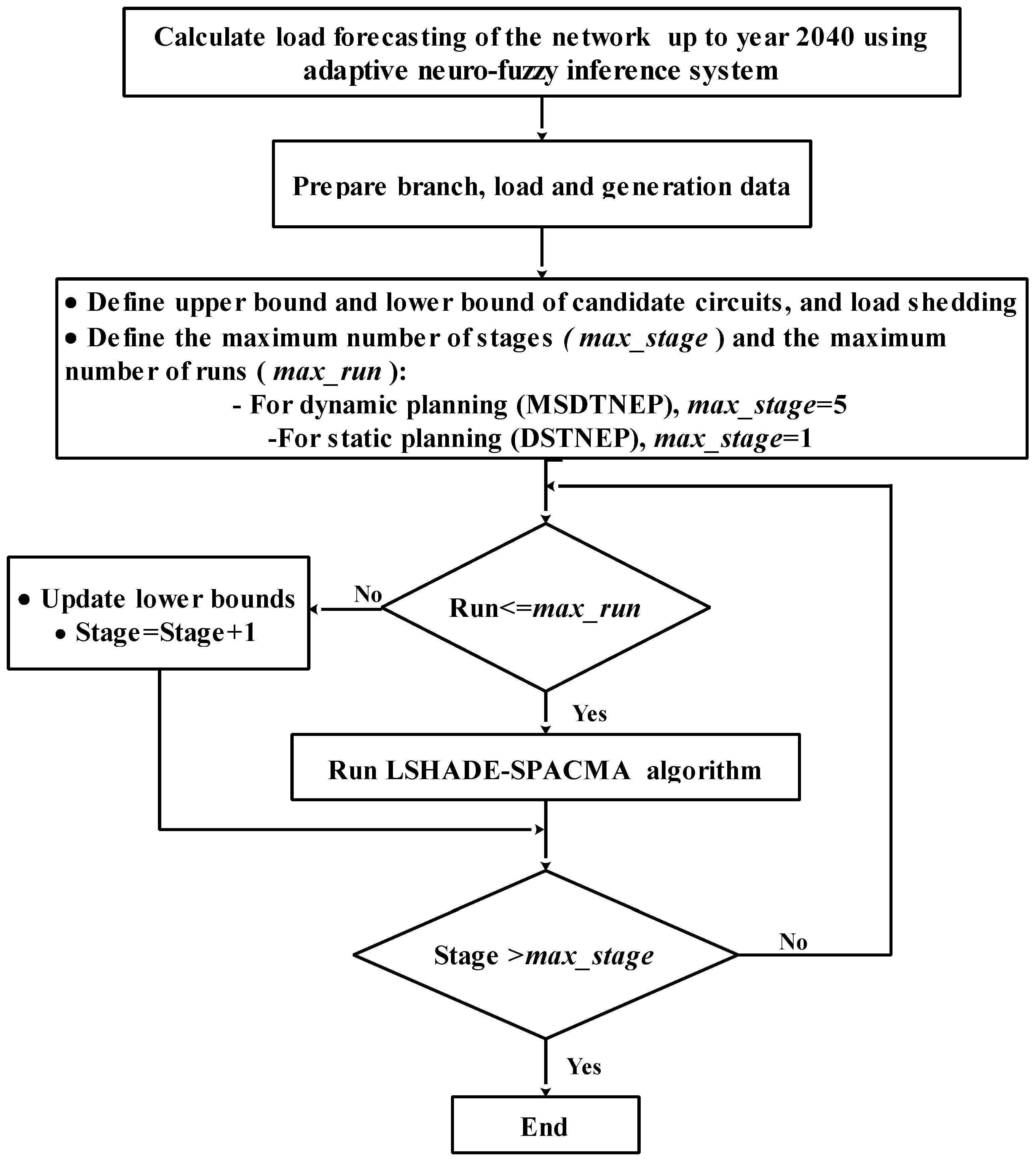
2.3. Applied Strategy

The proposed strategy to solve the TNEP problem (Figure 1) starts with an initial load forecast for WDN up to year 2040 using ANFIS. Next, the LSHADE-SPACMA algorithm was implemented to solve MSDTNEP and DSTNEP problems as long as the current run is less than or equal to the maximum number of runs (max_run). If the current run exceeded the max_run, both the lower bound and stage number were updated. This process was repeated until the current stage exceeded the maximum number of stages (max_stage). The max_stage for MSDTNEP and DSTNEP were 5 and 1, respectively.

3. Load Forecasting Using ANFIS

The ANFIS was used to obtain long-term load forecasting of WDN up to year 2040. Artificial intelligence techniques such as the fuzzy logic controller (FLC) and the artificial neural network (ANN) are commonly used in long-term load forecasting [24,25,26,27,28,29].
Recognizing the non-linear relationship between the selected input and the given output is the FLC’s key benefit in many applications in diverse fields. ANNs can “learn” because of the versatility of neuron-linking weights; thus, the solution can be adapted to boost efficiency. ANFIS combines ANN and FLC to enable this hybrid approach to adapt to various problems through machine learning using an iterative mechanism to detect non-linear relationships. ANFIS rapidly overcomes the complexities and robustness of the system by modeling its non-linear function with reasonable precision. The basic steps of ANFIS for long-term load forecasting are summarized as follows:
Step 1:
Define the input and output of the model. Input is the historical year and output is the actual peak load data.
Step 2:
Collect all data from previous periods and normalize scales,
Step 3:
Divide data into two sets—training data and test data. Training data are about 70–90% of the data available.
Step 4:
Run and estimate all reasonable ANFIS and determine the type of membership function and number of linguistic variables.
Step 5:
Select the best ANFIS model.
Step 6:
Project input variables using an autoregressive model in years (defined for the future).
Step 7:
Predict total peak loads using selected ANFIS.

4. LSHADE with Semi-Parameter Adaptation Hybrid with CMA-ES

Differential Evolution (DE) is a stochastic population-based optimization algorithm, starting with randomly generated individuals that evolve through probabilistic operators such as recombination and mutation [30,31,32]. The efficiency of DE depends heavily on population size (Np), the chosen mutation and/or crossover strategy, the mutation-associated scale factor (F), and the recombination-associated crossover rate (Cr). Adaptive methods for online modification of control parameters during DE were explored to eliminate the need to tune the parameters. In the literature, novel mutation techniques were introduced.
In Mohamed et al. [26], a semi- parameter adaptation scheme was implemented to enhance LSHADE technique’s performance. Besides, a hybridization strategy between LSHADE-SPA and CMA-ES was presented and considered successful on a wide range of optimization issues. In this section, the specifics of LSHADE-SPACMA are summarized, which is a recent improvement of LSHADE and is introduced in Mohamed et al. [26].

4.1. LSHADE

4.1.1. Initialization

To initialize LSHADE, a population of candidate solutions (decision vectors) is generated randomly within the specified upper and lower bounds. The mth component of the decision vector was formulated by the following Equation [26]:
D m , k o = D m , L + r a n d ( 0 , 1 ) ( D m , u D m , L )
where rand (0, 1) returns a uniformly distributed random number in [0, 1] and superscript ‘o’ represents initialization. If ‘d’ is the dimension of decision vector, then k = 1, 2, …, Np and m = 1, 2, …, d.

4.1.2. Mutation

Different DE mutation strategies were considered to generate a mutant vector corresponding to each population member D k G . In Mohamed et al. [26], the ‘current-to-pbest/1’ strategy is used and given by:
m u k G = D k G + F k G ( D P b e s t G D k G ) + F ( D r 1 G D r 2 G )
The p-value here is a control parameter that is supposed to enhance exploitation and exploration processes. Random indices ( r 1 and r 2 ) were picked from the population’s concatenation with an external archive that houses parent vectors that have generated successful vectors. The scale factor F is a positive control parameter used to scale the difference vector.

4.1.3. Crossover

For each generation G, the target vector is combined with muG using Equation (17) to generate the trial vector u k , m G based on C r [26]:
u k , m G = { m u k , m G ,   i f   ( r a n d k , m C r   O R   m = m r a n d ) D k , m G  
where r a n d k m is a uniformly distributed random number in set [0, 1] and m r a n d is a uniformly distributed random integer in set [1, d] to ensure that at least one component of the trial vector is inherited from the mutant vector.

4.1.4. Selection Scheme

DE implements a greedy selection technique. It states that if and only if the trial vector u k G yields an as-good-as or better fitness function value than D k G , then u k G is set to D k G + 1 . Otherwise, the old vector D k G is reserved. The selection scheme for a minimization problem follows [26]:
D k G + 1 = { u k G , i f   ( f ( u k G ) f ( D k G ) ) D k G , o t h e r w i s e

4.1.5. Linear Population Size Reduction (LPSR)

Linear Population Size Reduction (LPSR) is employed to boost the efficiency of LSHADE-SPA. The population size of the LPSR will be reduced by linear function as follows [22,26,27]:
N G + 1 = r o u n d [ ( N m i n N i n i t M A X N F E ) N F E + N i n i t ]

4.1.6. Semi-Parameter Adaptation (SPA) of Scaling Factor (F) and Crossover Rate (Cr)

Parameter adjustments had a significant effect on the efficiency of DE. Each problem has appropriate values for each parameter. SPA for F and Cr is proposed in [26] and is implemented in this work. It consists of two parts, in which the first part is activated during the first half of the search, and the second part is activated during the second half.

First Part of SPA

SPA’s idea is focused on adapting Cr using original LSHADE adaptation when the current number of iterations is less than half of the maximum number of iterations. While the F parameter is tuned using uniform distribution randomly within a specific limit as given in Equation (20) [26].
F k = 0.45 + 0.1 r a n d
However, C r k values are adapted based on the following Equation [26]:
C r k = r a n d n ( M c r k , 0.1 )
where M c r k is a randomly chosen memory slot that stores successful means of preceding generations. The memory index k is randomly selected from the range [1, h]. h is the size of memory. All Mcr initial values are 0.5, and one memory slot Mcr is updated at the end of each generation using the arithmetic mean of C r k values, that succeed to generate new individuals.

Second Part of SPA

In this part, the adaptation is concentrated on F, and LSHADE adaptation is used to adjust the Fk parameter as follows [26]:
F k = r a n d c ( M F k , σ )
where σ is the standard deviation for Cauchy distribution and equals 0.1, M F is a memory slot randomly chosen to store successful means of preceding generations. One memory slot M F is modified using the Lehmer mean of F k values at the end of each generation to successfully generate new individuals. The F k value of the previous five generations of the first part of the SPA was used to initialize the memory slot M F for the second part of SPA. The Cr parameter adaptation process remains as is during the second part. However, due to the nature of the LSHADE parameter adaptation, the Cr parameter is gradually frozen to the adapted values. According to the SHADE parameter adaptation, when successful individuals do not produce all Cr values in a generation, the corresponding memory slot is adjusted to the terminal value. Therefore, MCr will not be updated until the search is over.

4.2. Covariance Matrix Adaptation Evolution Strategy (CMA-ES)

Among its many variants, CMA-ES can solve various types of optimization problems efficiently. In CMA-ES, a multivariate normal distribution is used to model the search space. New individuals are produced using Gaussian distribution that accounts for the population’s path over successive generations. CMA-ES automatically adapts the mean vector m, covariance matrix C, and step size σc. CMA-ES steps are summarized according to [26]:
  • Generate an initial population and then calculate the fitness function.
  • Gaussian distribution is used to produce new individuals, thus:
    D k = N ( T , σ c 2 C )     i = 1 , , n
  • Update m using the best μ individuals according to T = k = 1 μ W k   D k   ,   where k = 1 μ W k = 1 and   W 1 W 2 W μ .
  • Update σc and C.
  • Steps 2 and 3 are repeated until a stop criterion is met.

4.3. LSHADE-SPACMA Hybridization Framework

In order to enhance LSHADE-SPA’s performance, a hybridization framework between the recent version of CMA-ES and LSHADE-SPA is applied [26]. Each individual D in the population produces an individual u offspring using either LSHADE or CMA-ES according to the probability variable (FCP) class. FCP values are chosen randomly from memory slots that are set to MFCP. One memory slot is modified at the end of each generation based on the output of each algorithm. As a result, populations were gradually assigned to a better performance algorithm. Updates were produced using individuals that successfully created new individuals. The memory slot of the MFCP is then updated based on the following formula:
M F C P , G + 1 = ( 1 C ) M F C P , G + C   A l G 1
where C is the learning rate, and A l G 1 is the improvement rate for each algorithm calculated according to Equation (25):
A l G 1 = m i n ( p r o b m a x , m a x ( p r o b m i n , ω A l G 1 ω A l G 1 + ω A l G 2 )
where p r o b m i n and p r o b m a x are the minimum and maximum probabilities set to each algorithm, respectively. Thus, to execute both algorithms together, FCP values must be maintained in the range of 0.2 to 0.8. The variable ω A l G 1 is the summation of differences between the old and new fitness values for each individual belonging to the algorithm in Equation (26):
ω A l G 1 = i = 1 n f ( u o l d ) f ( u ) ,
where f is the fitness function. u o l d and u are the old and the offspring individuals, respectively. n is the number of individuals belonging to algorithm A l G 1 .

4.4. Pseudocode of LSHADE-SPACMA for Solving the TNEP Problem

The pseudocode of the LSHADE-SPACMA algorithm for solving the TNEP problem is presented in Table 1. It starts with setting the population size and dimension of the problem and defining the maximum number of problem evaluations, the lower bound, and the upper bound of decision variables. The population of Np individuals was initialized according to Equation (15), and initial values of SHADE and CMA control parameters were introduced. Steps 1 through 10 are repeated until a stop criterion is reached.

5. Simulation Results and Analyses

An assessment of three standard test systems—Garver 6-bus test system, Egyptian WDN, and 93-bus Colombian system—were carried out to verify the proposed optimization technique’s capability to solve the TNEP problem. Static plan results, using LSHADE-SPACMA, were compared to results obtained in previous studies [4,13,20,21,28]. Finally, MSDTNEP of WDN up to 2040 with embedded N-1 security constraints is employed based on two scenarios. The following case studies are conducted on MATLAB r2017a on a DELL PC, and its model name is ‘OptiPlex7050‘, including an ‘Intel® Core™ i7’ CPU at 2.6 GHz and 16 GB RAM.

5.1. Validation of LSHADE-SPACMA Technique to Solve the TNEP Problem

5.1.1. Garver 6-Bus Test System

In the pioneering paper [4], the Garver network was discussed and has since been used by many other researchers to compare various TNEP approaches. Figure 2 shows that it comprises 6 buses and 6 lines. Bus 6 is not connected to the rest of the network in the initial configuration, and the current demand for buses 1–5 is 760 MW, while the installed generation capacity for these interconnected nodes is only 215 MW. As a result, to avoid power from not being supplied, the TNEP would have to facilitate interconnecting bus 6 to the rest of the network.
Regarding the standard Garver system, it is important to stress that the optimal identified solution is the same as the solution mentioned in the literature to validate the proposed algorithm’s efficiency in solving the TNEP problem. The final configuration and the optimal solution of TNEP for the Garver 6-bus network system using the LSHADE-SPACMA technique are depicted in Table 2 and Figure 2b. This solution includes one new branch between nodes 3 and 5, two new branches between nodes 4 and 6, and four new branches between nodes 2 and 6. The proposed method gives 13 paths with costs of 200 million USD. It provides the same results obtained by Garver [4] using the linear programming (LP) method in 6.68 s, decreasing the computational burden.

5.1.2. 93-Bus Colombian System

The Colombian test system had 93 buses and 155 circuits. It was designed to meet a 9750 MW load system, and 155 control variables were optimized to minimize the total investment cost. The initial configuration for the system can be seen in Escobar et al. [17].
The best topology for the Colombian system using LSHADE-SPACMA is depicted in Table 3, which produced the same results obtained by Escobar et al. [13]. Both methods added 6 circuits at an investment cost of 316.44 million USD, while LSHADE-SPACMA got the global optimum solution in 475.19 s. The results demonstrate that LSHADE-SPACMA is sufficient to solve large-scale systems and complex problems in one run.

5.2. West Delta Network (WDN) System Planning

WDN is a 66 kV transmission network and a section of the Unified Egyptian Network. The initial configuration of WDN with proposed routes is shown in Figure 3 [24]. It comprises a 52-bus system connected by 55 double circuits, 8 generation units, and 44 load buses. The actual data of WDN are introduced in [24].

5.2.1. Validation of LSHADE-SPACMA Technique to Solve the TNEP Problem for WDN

WDN was expected to meet the predicted peak load of the 2195.8 MW. A new site generator at bus 53 and 31 candidate routes have been proposed [24,25,33]. The new configuration of WDN is shown in Table 4. LSHADE-SPACMA adds seven new right of way routes and yields 17.28 million USD for an investment cost of the added transmission lines, and the consumed time of one run is 164.78 s. The results demonstrate, moreover, that LSHADE-SPACMA has the superiority compared to the HM [33], IBPSO [24], and MVO [25], because they acquired a high investment cost of 21.24, 22.19, and 20.645 million USD, respectively. The results presented in Table 5 explore that the power flow in the transmission lines is within its prescribed limits.

5.2.2. Multi-Stage Dynamic Planning for WDN up to 2040 without Security N-1 Security Constraint

In this section, MSDTNEP of WDN without N-1 security constraint is employed up to year 2040. The actual peak load data of WDN from the year 2008 to 2015 are used in the load forecasting process [24]. The load forecasting up to year 2040 using ANFIS, linear, parabolic and exponential trends is presented in Figure 4. The results show that ANFIS has the lowest mean absolute error (MAE) and the best results; therefore, it is applied in this work. The predicted loads from 2016 to 2040 using ANFIS are shown in Table 6.
MSDTNEP without including an N-1 security constraint for WDN from 2016 up to 2040 is shown in Table 7. The planning period is divided into five stages and each stage comprises five years. The considered interest rate is 0.2. The dynamic planning results in adding three circuits in the first and second stages, two circuits in the third stage, and four circuits in the fourth and fifth stages to guarantee that the power system operates economically and reliably. The results also show that the generation station’s capacity at bus 53 should be increased to 1315.7 MW to meet the possible load demand in 2040. Dynamic planning of WDN in 2030 (third stage) shows that total circuits added from 2016 to 2030 are eight; however, the static plan in Section 5.2.1 gives seven circuits. As in dynamic planning, each stage depends on previous stages. In the second and third stages, six new routes are added to ensure reliable operation for the power system and meet each bus’s load demand in these periods. Hence, these routes are imposed in the planning of the third stage.

5.2.3. Multi-Stage Dynamic Planning for WDN up to 2040 with Security N-1 Security Constraint

To study the impact of including N-1 security constraint on WDN planning, two scenarios were suggested to keep the power system reliable, secure, and low cost:
Scenario 1: The system was planned with the same routes proposed in Fathy et al. [24] and load shedding was applied.
Scenario 2: The maximum number of circuits in each route was supposed to be four, as per Egyptian requirements.
Table 8 and Figure 5 show that the planning of WDN with routes proposed by Fathy et al. [24] for scenario 1 cannot ensure system security without load shedding. Scenario 1 results in the addition of 15 circuits with load shedding of 162.68 MW in the first stage, 6 circuits with load shedding of 43.23 MW in the second stage, 1 circuit with load shedding of 127.4 MW in the third stage, 4 circuits with load shedding of 134.19 MW in the fourth stage, and 5 circuits with load shedding of 160.46 MW in the fifth stage. The total investment cost would be 287.46 million USD.
Scenario 2 proposes 25 circuits in the first stage, 8 circuits in the second stage, 20 circuits in the third stage, 7 circuits in the fourth stage, and 12 circuits in the fifth stage, as depicted in Table 8 and Figure 6. The total investment cost is 57.33 million USD, lower than scenario 1. Hence, scenario 2 is recommended.
It is clear that steady-state power system insecurity based on scenario 1 overloads transmission lines and causes successive interruptions leading to partial blackouts (Figure 7 and Table 8). The results demonstrate that increasing the capacity at bus 53 cannot mitigate the rolling blackout problem, and the available solution is to install distribution generators at various locations, causing the total investment cost to increase. On the other hand, MSDTNEP of WDN based on scenario 2 leads to a better plan for WDN and lower investment cost, because it accounts for several features such as annual load growth, prevention of rolling blackouts, and N-1 security criterion. Blackouts are avoided in scenario 2 by installing additional circuits of lower cost compared to the cost of installing new distribution generators (Figure 7).

6. Conclusions and Future Works

The implementation of the LSHADE-SPACMA algorithm was investigated to solve the TNEP problem. Promising results were obtained using three sample systems and confirmed the potential of this approach. The results show that the LSHADE-SPACMA algorithm produces a better (low-cost) solution than IBPSO, MVO, and HT for the WDN. Moreover, the LSHADE-SPACMA reached optimum solutions for both large- and small-scale systems such as the Colombian system and the Garver test system in a single run.
Ignoring N-1 reliability constraint in the TNEP model threatens the security of power systems. A suggested approach to tackle this problem was applied to the Egyptian WDN, and its performance was evaluated. The MSDTNEP up to year 2040 including an N-1 security constraint, and it was assessed based on two scenarios. Scenario 1 adopted plans based on the candidate routes with the implementation of load shedding. Scenario 2, the suggested solution, assumed that the maximum number of circuits in each line could be increased to 4.
ANFIS was employed to predict load demand growth until 2040. The input and the output of ANFIS are the historical year and the actual peak load data, respectively. The numerical results show that dynamic planning leads to a more accurate and realistic assessment of the network. Moreover, the N-1 security constraint has a significant impact on the final configuration of WDN. The results also demonstrate that the planning of WDN with the candidate lines proposed in scenario 1 cannot guarantee system security without imposing a load shedding or partial blackouts. It should be noted that scenario 1 results in the addition of 31 circuits with load shedding of 627.96 MW at the end of the planning horizon. The total investment cost is estimated to be 287.46 million USD. Scenario 2 does not cause blackouts and is recommended. This scenario requires the addition of 62 circuits with no load shedding and an investment cost of 57.33 million USD.
The results demonstrated that the suggested strategy is considered a promising solution to maintain N-1 security and avoid rolling blackouts. It is applicable for all power systems because it is not complex and has a low investment cost [34].
Egypt’s vision is to achieve an energy sector that meets national sustainable development standards and optimizes the use of renewable resources to support economic growth and protect the environment’s health and quality [35,36]. Hence, a new paradigm of transmission and generation planning for WDN is needed, which considers the system’s increasingly decentralized and stochastic nature due to the predicted high penetration of renewable energy sources in the Egyptian network.

Author Contributions

M.M.R. and S.H.E.A.A. designed the problem under study; M.M.R. performed the simulations and obtained the results; S.H.E.A.A. analyzed the obtained results; M.M.R. wrote the paper, which was further reviewed by S.H.E.A.A., Y.A., M.M.S., and Z.M.A. All authors have read and agreed to the published version of the manuscript.

Funding

This research received no external funding.

Institutional Review Board Statement

Not applicable.

Informed Consent Statement

Not applicable.

Data Availability Statement

The data presented in this study are available on request from the corresponding author. The data are not publicly available due to their large size.

Conflicts of Interest

The authors declare no conflict of interest.

Nomenclature

Input Data and Indices
ACTNEPAC transmission network expansion planning
ANFISAdaptive neuro-fuzzy inference system
CMA-ESCovariance Matrix Adaptation Evolution Strategy
DCTNEPDC transmission network Expansion planning
DCPFDC power flow
DEDifferential Evolution
DSTNEPDeterministic static transmission network expansion planning
DTNEPDynamic transmission network expansion planning
GAGenetic algorithm
HMHeuristic method
LPLinear programming
LPSRLinear population size reduction
LSHADE-SPACMALinear population size reduction Success History-based Differential Evolution with semi-parameter adaptation hybrid with CMA-ES
MSDTNEPMulti-stage dynamic transmission network expansion planning
SPASemi-parameter adaptation
STNEPStatic transmission network expansion planning
TNEPTransmission network expansion planning
WDNEgyptian West Delta Network
RLine resistance
P i Active power injection at bus i
BijSusceptance of route between bus i and j
θ i , θ j Voltage angles at bus i and j, respectively
P G i , P d i Active power generation source and the load demand (MW) at bus i, respectively
C i j Cost of circuit between buses i and j
XLine reactance
X i j 0 ,   X i j _ m a x , X i j Initial number of circuits, the maximum number of circuits, and the actual number of circuits between buses i and j, respectively
P i j , P i j _ m a x Active power flow and the active power flow limit in the i-j right of way (MW), respectively
P s h , i Amount of load shedding
C r Penalty parameter that penalizes, in the objective function, any system load shedding
α Maximum percentage of load shedding
N y ,   y r Total number of stages and stage number, respectively
NpPopulation size
D m , k o , D m , u , D m , L Initial, upper bound, and lower bound of mth component of the decision vector, respectively
m u k G Mutant vector corresponding to each population member D k G
FScale factor
CRCrossover rate
D Pbest G Best individual vector with the best fitness value at G generation in the population
u k , m G Trial vector
NFECurrent number of fitness evaluations
MAXNFEMaximum number of fitness evaluations
NinitInitial population size
NminMinimum number of individuals that DE can work with

References

  1. Mahdavi, M.; Antunez, C.S.; Ajalli, M.; Romero, R. Transmission expansion planning: Literature review and classification. IEEE Syst. J. 2019, 13, 3129–3140. [Google Scholar] [CrossRef]
  2. Freitas, P.F.S.; Macedo, L.H.; Romero, R. A strategy for transmission network expansion planning considering multiple generation scenarios. Elect. Power Syst. Res. 2019, 172, 22–31. [Google Scholar] [CrossRef]
  3. Naderi, E.; Pourakbari-Kasmaei, M.; Lehtonen, M. transmission expansion planning integrated with wind farms: A review, comparative study, and a novel profound search approach. Int. J. Electr. Power Energy Syst. 2020, 115, 105460. [Google Scholar] [CrossRef]
  4. Garver, L.L. Transmission Network Estimation. IEEE Trans. Power Appar. Sys. 1970, 89, 1688–1697. [Google Scholar] [CrossRef]
  5. Han, S.; Kim, H.-J.; Lee, D. A Long-term evaluation on transmission line expansion planning with multistage stochastic programming. Energies 2020, 13, 1899. [Google Scholar] [CrossRef] [Green Version]
  6. Taherkhani, M.; Hosseini, S.H.; Javadi, M.S.; Catalão, J.P. Scenario-based probabilistic multi-stage optimization for transmission expansion planning incorporating wind generation integration. Elect. Power Syst. Res. 2020, 189, 106601. [Google Scholar] [CrossRef]
  7. Zhang, F.; Hu, Z.; Song, Y. Mixed-integer linear model for transmission expansion planning with line losses and energy storage systems. IET Gener. Transm. Distr. 2013, 7, 919–928. [Google Scholar] [CrossRef]
  8. Dodu, J.C.; Merlin, A. Dynamic model for long-term expansion planning studies of power transmission systems: The Ortie model. Int. J. Elect. Power Energy Syst. 1981, 3, 2–16. [Google Scholar] [CrossRef]
  9. Mora, C.A.; Montoya, O.D.; Trujillo, E.R. Mixed-integer programming model for transmission network expansion planning with battery energy storage systems (BESS). Energies 2020, 13, 4386. [Google Scholar] [CrossRef]
  10. Li, Y.-H.; Wang, J.-X. Flexible transmission network expansion planning considering uncertain renewable generation and load demand based on hybrid clustering analysis. Appl. Sci. 2016, 6, 3. [Google Scholar] [CrossRef] [Green Version]
  11. Das, S.; Verma, A.; Bijwe, P.R. Efficient multi-year security constrained AC transmission network expansion planning. Elect. Power Syst. Res. 2020, 187, 106507. [Google Scholar] [CrossRef]
  12. Lee, S.T.Y.; Hicks, K.L.; Hnyilicza, E. Transmission expansion by branch-and-bound integer programming with optimal cost-capacity curves. IEEE Trans. Power Appar. Syst. 1974, PAS-93, 1390–1400. [Google Scholar] [CrossRef]
  13. Zhan, J.; Chung, C.Y.; Zare, A. A fast solution method for stochastic transmission expansion planning. IEEE Trans. Power Syst. 2017, 32, 4684–4695. [Google Scholar] [CrossRef]
  14. Pereira, M.V.F.; Pinto, L.M.V.G. Application of sensitivity analysis of load supplying capability to interactive transmission expansion planning. IEEE Trans. Power Appar. Syst. 1985, 381–389. [Google Scholar] [CrossRef]
  15. Sousa, A.S.; Asada, E.N. Combined heuristic with fuzzy system to transmission system expansion planning. Elect. Power Syst. Res. 2011, 81, 123–128. [Google Scholar] [CrossRef]
  16. Da Silva, E.L.; Gil, H.A.; Areiza, J.M. Transmission network expansion planning under an improved genetic algorithm. IEEE Trans. Power Syst. 2000, 15, 1168–1174. [Google Scholar] [CrossRef]
  17. Escobar, A.H.; Gallego, R.A.; Romero, R. Multistage and coordinated planning of the expansion of transmission systems. IEEE Trans. Power Syst. 2004, 19, 735–744. [Google Scholar] [CrossRef]
  18. Da Silva, E.L.; Ortiz, J.M.A.; De Oliveira, G.C.; Binato, S. Transmission network expansion planning under a tabu search approach. IEEE Trans. Power Syst. 2001, 16, 62–68. [Google Scholar] [CrossRef]
  19. Binato, S.; De Oliveira, G.C.; De Araújo, J.L. A greedy randomized adaptive search procedure for transmission expansion planning. IEEE Trans. Power Syst. 2001, 16, 247–253. [Google Scholar] [CrossRef]
  20. Shayeghi, H.; Mahdavi, M.; Bagheri, A. Discrete PSO algorithm based optimization of transmission lines loading in TNEP problem. Energy Convers. Manag. 2010, 51, 112–121. [Google Scholar] [CrossRef]
  21. Shayeghi, H.; Mahdavi, M.; Bagheri, A. An improved DPSO with mutation based on similarity algorithm for optimization of transmission lines loading. Energy Convers. Manag. 2010, 51, 2715–2723. [Google Scholar] [CrossRef]
  22. Torres, S.P.; Castro, C.A. Expansion planning for smart transmission grids using AC model and shunt compensation. IET Gener. Transm. Distr. 2014, 8, 966–975. [Google Scholar] [CrossRef]
  23. Huang, S.; Dinavahi, V. Multi-group particle swarm optimisation for transmission expansion planning solution based on LU decomposition. IET Gener. Transm. Distr. 2017, 11, 1434–1442. [Google Scholar] [CrossRef]
  24. Fathy, A.A.; Elbages, M.S.; El-Sehiemy, R.A.; Bendary, F.M. Static transmission expansion planning for realistic networks in Egypt. Elect. Power Syst. Res. 2017, 151, 404–418. [Google Scholar] [CrossRef]
  25. Shaheen, A.M. Application of multi-verse optimizer for transmission network expansion planning in power systems. In Proceedings of the 2019 International Conference on Innovative Trends in Computer Engineering (ITCE’2019), Aswan, Egypt, 2–4 February 2019. [Google Scholar]
  26. Mohamed, A.W.; Hadi, A.A.; Fattouh, A.M.; Jambi, K.M. LSHADE with Semi-Parameter Adaptation Hybrid with CMA-ES for Solving CEC 2017 Benchmark Problems. In Proceedings of the 2017 IEEE Congress On Evolutionary Computation (Cec), San Sebastián, Spain, 5–8 June 2017. [Google Scholar]
  27. Nazar, M.S.; Vahidi, B.; Hosseinian, S.H. TNEP and the effects of wind generation on market prices, network reliability, and line failures in TNEP. Int. J. Electr. Power Energy Syst. 2020, 123, 106296. [Google Scholar] [CrossRef]
  28. Silva, I.D.J.; Rider, M.J.; Romero, R.; Garcia, A.V.; Murari, C.A. Transmission network expansion planning with security constraints. IET Gener. Transm. Distr. 2005, 152, 828–836. [Google Scholar] [CrossRef]
  29. Akdemir, B.; Çetinkaya, N. Long-term load forecasting based on adaptive neural fuzzy inference system using real energy data. Energy Procedia 2012, 14, 794–799. [Google Scholar] [CrossRef] [Green Version]
  30. Tanabe, R.; Fukunaga, A.S. Improving the search performance of SHADE using linear population size reduction. In Proceedings of the 2014 IEEE Congress on Evolutionary Computation (CEC), Beijing, China, 6–11 July 2014. [Google Scholar]
  31. Fathy, A.; Aleem, S.H.E.A.; Rezk, H. A novel approach for PEM fuel cell parameter estimation using LSHADEEpSin optimization algorithm. Int. J. Energy Res. 2020, 1–21. [Google Scholar] [CrossRef]
  32. Zhang, J.; Member, S.; Sanderson, A.C. JADE: Adaptive differential evolution with optional external archive. IEEE Trans. on Evolutionary Comp. 2009, 13, 945–958. [Google Scholar] [CrossRef]
  33. Fathy, A.A.; Elbages, M.S.; Mahmoud, H.M.; Bendary, F.M. Transmission expansion planning for realistic Network in Egypt using Heuristic Technique. Int. Electrical Eng. J. 2016, 7, 2148–2155. [Google Scholar]
  34. Zobaa, A.F.; Aleem, S.H.E.A.; Abdelaziz, A.Y. Classical and Recent Aspects of Power System Optimization; Academic Press: Cambridge, MA, USA; Elsevier: Amsterdam, The Netherlands, 2018. [Google Scholar]
  35. Abdel Aleem, S.H.E.; Zobaa, A.F.; Abdel Mageed, H.M. Assessment of energy credits for the enhancement of the Egyptian Green Pyramid Rating System. Energy Policy 2015, 87, 407–416. [Google Scholar] [CrossRef] [Green Version]
  36. Rawa, M.; Abusorrah, A.; Al-Turki, Y.; Mekhilef, S.; Mostafa, M.H.; Ali, Z.M.; Aleem, S.H.E.A. Optimal allocation and economic analysis of battery energy storage systems: Self-consumption rate and hosting capacity enhancement for microgrids with high renewable penetration. Sustainability 2020, 12, 144. [Google Scholar] [CrossRef]
Figure 1. Proposed strategy to solve transmission network expansion planning (TNEP) problem.
Applsci 11 02155 g001
Figure 2. Garver system: (a) New configuration using LSHADE-SPACMA; (b) New configuration using LP [4].
Applsci 11 02155 g002
Figure 3. Single-line diagram of WDN [24].
Applsci 11 02155 g003
Figure 4. WDN load forecasting using ANFIS, linear, parabola and exponential trends.
Applsci 11 02155 g004
Figure 5. Optimal configuration for WDN based on scenario 1.
Applsci 11 02155 g005
Figure 6. Optimal configuration for WDN based on scenario 2.
Applsci 11 02155 g006
Figure 7. Comparison between scenarios 1 and 2.
Applsci 11 02155 g007
Table 1. Pseudo-code of LSHADE-SPACMA algorithm to solve the TNEP problem.
Input
  • Dimension of the problem, d.
  • Population size, Np.
  • Stop criterion, MAXNFE (i.e., maximum number of fitness evaluations).
  • Maximum and minimum values of d-decision variables, in vector form Dmax and Dmin.
xmax = [Dmax,1, …, Dmax,d] and xmin = [Dmin,1, …, Dmin,d ].
Initialization
  • Set generation counter, t = 1 and function evaluation counter NFE = 0.
  • Set SHADE parameters: Memory M size, initialize MFcP = 0.5, MCr = 0.5 and MF = 0.5.
  • POP: Create a population of Np individuals according to Equation (14).
  • Initialize CMA parameters.
  • Evaluate objective function and constraint violation using Equation (2) to Equation (6) or using Equation (7) to Equation (14) for each individual in POP.
  • Increase function evaluation counter NFE by Np.
Algorithm loop
Step 1 For i = 1:NP, do
ri = select from [1,H] randomly;
C r i , G = r a n d n ( M c r i , 0.1 )
FCPi,g = MFCP,ri
If nfes < max_nfes/2
F i , G = 0.45 + 0.1 r a n d ;
otherwise,
F i , G = r a n d n ( M f r i , 0.1 ) ;
end
end
Step 2
  • Generate donor vector using LSHADE ( V L S H A D E ).
  • Generate donor vector using CMA ( V C M A ).
  • Concatenate V L S H A D E , V C M A .
Step 3Generate trial vector (U).
Step 4
  • Check constraints from Equations (3)–(6) or (8)–(14).
  • Evaluate (U) using fitness Equations (2) or (7).
Step 5Update POP and Fitness function according to the evaluation of U.
Step 6Store successful FCP, F, and Cr
Step 7
  • Update archive A
  • If (archive size >   | A | )
Delete individuals archive randomly
End
Step 8Update MCr and MFCP
If nfes < max_nfes/2
Update MF
end
Step 9
  • Calculate NG+1 according to Equation (19).
  • If NG < NG+1
-
Sort individuals in P based on their fitness values and delete the NG-NG+1 member.
-
Resize archive ( | A | ) according to the new POP.
End
Step 10
  • Update CMA parameters.
Table 2. New configurations of Garver network using LP [4] and LSHADE-SPACMA.
Optimization Algorithm
LP [4]LSHADE-SPACMA
TerminalNo. of CircuitsPower Flow
(MW)
TerminalNo. of CircuitsPower Flow
(MW)
FromToFromTo
121−51121−51.25
141−32141−31.74
1515315152.99
2316223162.00
24142413.63
352187352187.00
263−357264−356.88
463−188462−188.12
Cost
(million USD)
200Cost
(million USD)
200
Time (s)NC *Time (s)6.68
* NC donates not calculated.
Table 3. New configuration of the Colombian system presented in Escobar et al. [13] and LSHADE-SPACMA.
Escobar et al. [17]LSHADE-SPACMA
TerminalNo. of CircuitsTerminalNo. of Circuits
FromToFromTo
4581145811
5557155571
5562155621
5657156571
5681156811
8285182851
Cost
(million USD)
316.44Cost
(million USD)
316.44
Time (s)NCTime (s)475.19
Table 4. New right-of-way routes and transmission line costs for WDN using IBPSO, HT, MVO, and LSHADE-SPACMA.
IBPSO [20]HT [28]MVO [21]LSHADE-SPACMA
TerminalNo. of CircuitsTerminalNo. CircuitsTerminalNo. CircuitsTerminalNo. of Circuits
FromToFromToFromToFromTo
522163426341561
634231531736133531
3353232531225315532
34532335313753136532
36532345313353120531
3553134531
3653236532
Added circuits9Added circuits9Added circuits8Added circuits7
Total Cost
(million USD)
22.19Total Cost
(million USD)
21.24Total Cost
(million USD)
20.64Total Cost
(million USD)
17.28
Time (s)NCTime (s)NCTime (s)NCTime (s)164.78
Table 5. Power flow injection in the new configuration of WDN.
LSHADE-SPACMA
TerminalNo. CircuitsPower Flow
(MW)
Max. Power Flow
(MW)
TerminalNo. CircuitsPower Flow
(MW)
Max. Power Flow
(MW)
FromToFromTo
6412210.36278.082829227.13175.52
41392112.38175.52132923.51175.52
3938227.6787.7922132137.23278.08
8412−73.13278.0813302114.53175.52
851214.4822112240.68292.64
846274.95175.522122−26.56278.08
8472161.11278.08425224.9343.84
47482105.77175.52424223.4843.84
4849277.65175.52242521.6043.84
317271.61278.0842327.05278.08
1719236.71175.52426258.17175.52
316252.18278.083142−52.27278.08
1618247.94278.0823142−12.71278.08
111295.88175.522021250.17278.08
1128285.72175.5218202−4.79278.08
7432185.89278.08642291.80278.08
44432−81.42175.52214275.20278.08
44452−3.29175.52315212.71278.08
7422−19.7782.3042122219.76278.08
404225.9082.304427228.24278.08
640266.6182.304110222.5987.792
6362−163.09175.5219215.4487.792
536299.07175.524950216.9487.792
533213.4487.7925152211.29175.52
3635263.3987.792537233.8887.792
534259.66175.52561131.08139.04
531242.45278.0833531−97.36139.04
31302−43.09175.525532−188.29278.08
3032260.14278.0836532−276.58278.08
4645217.41175.5220531−77.55139.04
Total number of circuits = 117
Table 6. Load forecasting for WDN using ANFIS technique up to year 2040.
YearPredicted LoadYearPredicted Load
20161260.220292128.3
20171325.120302195.8
20181390.620312263.4
20191456.620322330.9
2020152320332398.5
20211589.720342466.1
20221656.720352533.7
20231723.820362601.3
2024179120372668.9
20251858.420382736.5
20261925.820392804.1
20271993.220402871.7
20282060.7
Table 7. Dynamic planning of WDN up to 2040 without N-1 security.
Stage No.Added LinesTotal Cost
(Million USD)
5–65–86–347–347–3623–5322–5333–535–5334–5336–538–53
1001 *0010010004.71
21010010110107.23
31010010121203.42
41111010122206.28
51111111122226.58
Total circuits = 12628.22
* Grey shading indicates a change in the number of circuits.
Table 8. Dynamic planning of WDN up to year 2040 with N-1 security.
Candidate LineScenario 1Candidate LineScenario 2
Stage NumberStage Number
1234512345
5–6111116–4100222
5–71111141–3902222
5–81111139–3812222
5–22111118–4122222
5–29111118–5111222
5–32000018–4700222
6–320000147–4802222
6–341111148–4900011
6–37000013–1700002
7–32011117–4311111
7–331111144–4322222
7–340001144–4500222
7–36111117–4211222
7–37001116–36000 11
8–38111115–3612222
8–33000115–3322222
8–341111136–3522222
8–360111113–2922222
8–371111113–3022222
25–53000114–2400002
23–531111124–2500002
22–53000114–2600222
19–531111118–2022222
37–53000016–4211111
33–53011112–1400011
5–53011111–1000222
31–53011111–900002
34–53000015–3700001
36–53111115–711112
20–53111115–800111
8–53011115–2200444
NA *6–3211111
6–3400122
23–5311111
22–5300111
33–5300001
5–5324444
34–5300111
36–5300034
Added circuits156145 25820712
Added load shedding (MW)162.6843.23127.4134.19160.46 00000
Cost
(million USD)
115.0736.2546.1144.3945.63 25.77.738.126.596.16
* NA denotes not applicable.
Publisher’s Note: MDPI stays neutral with regard to jurisdictional claims in published maps and institutional affiliations.

