Baselining Flexibility from PV on the DSO-Aggregator Interface

Abstract

Flexibility can be used to mitigate distribution network overloading. Distribution system operators (DSOs) can obtain this flexibility from market parties connected to the distribution network. After flexibility has been delivered to the DSO, it needs to be settled. This is typically done by comparing load measurements with a baseline. This baseline describes an asset’s power profile in case no flexibility would have been delivered. Until recently, baselining research mainly focused on large-scale, predictable and controllable assets. The flexibility used by DSOs however typically comes from small-scale, less predictable and less controllable assets. This paper addresses the baselining problem for photo-voltaic systems. Three existing baselining methods are selected based on their simplicity and transparency and their limitations with respect to application towards photo-voltaic systems are evaluated. Based on this, a proof-of-concept for a new, fourth method is provided. It overcomes some of the limitations of the three existing ones, while still ensuring simplicity and transparency in order to promote market acceptance and practical applicability. All four methods are subjected to two different curtailment strategies: curtailing all peaks above a threshold and curtailing based on a day-ahead flexibility request. Using weather data from three summer weeks in 2019, it is shown that the newly developed method is able to provide a more accurate baseline than the existing methods.

1. Introduction

As the energy transition is gaining momentum, more and more photo-voltaic (PV) and wind turbines are connected to the distribution networks. Furthermore, fossil-fuel based heating and transportation is being replaced by electric alternatives, such as heat pumps (HPs) and electric vehicles (EVs). Distributed energy resources (DERs) strain the existing distribution networks, which have not been designed for the peak loads caused by these new technologies. When a high penetration of DERs is expected, distribution system operators (DSOs) must reinforce their networks to avoid network congestion (overloading). Since large-scale reinforcements are costly and time-consuming, the need for alternatives to prevent or postpone reinforcements is urgent. One of the promising alternatives is the use of demand response (DR) in order to utilise flexibility.

Both research and pilot projects have shown DR can be used as a mitigation measure for expected congestion in distribution networks. Reviews of a number of DR projects are provided by [1,2], where [1] places four pilot projects in the perspective of the current European regulations and [2] analyses the viability of four different DR mechanisms related to a pilot project in the Netherlands. In the unbundled energy sector of Europe, characterised by a strict distinction between network operation on one hand and electricity generation and consumption on the other, DSOs must rely on third parties to provide DR services. These third parties should receive adequate compensation. It is therefore necessary for both DSOs and third parties to be able to verify the delivered flexibility. This is typically done using a so-called baseline, which describes the behaviour of an asset in case no DR service would have been provided.

Baselining is identified as one of the main barriers in the deployment and evaluation of DR. According to [3], accurate baselines are needed in order to enable DR in Europe. To achieve this, the availability of measurements and historical baselines is required. A more in-depth discussion of baselining can be found in [4]. A baseline forms a synthetic and hypothesised profile, and therefore per definition has an error. This observation is seen as a threat to consumer’s participation to a DR program, as the (financial) compensation of flexibility provided depends on the accuracy of the baseline. It is furthermore argued that although baselining is already applied for (large) industrial and commercial loads, providing an accurate baseline for smaller devices with irregular consumption might be a challenge [4]. The work of [5] takes the transmission system perspective of deploying flexibility, analysing operational planning, operations, and settlement. As part of their analysis, [5] identifies the lack of an appropriate baselining methodology as the most urgent barrier for aggregators to provide balancing services.

Numerous authors have pointed out the necessity of truth-telling in DR schemes. Chen analysed a DR program from a game theoretical perspective [6]. The DR program is tested for its truth-telling and cheat-proof behaviour. The authors show the need for truth-telling in a distributed solution, with consumers behaving naturally selfish. The universal smart energy framework (USEF) foundation identifies gaming as one of the issues with their (self-reported) baseline model, in which deviations from the reported baseline are not penalised [7,8]. In [9], a DR program is implemented, taking the system operator’s perspective. Consumers report their baseline and to ensure truth-telling, consumers deviating from the baseline—while not providing promised flexibility—are penalised with a random penalty. An alternative implementation of this DR program uses a reported baseline in which consumers not only provide their baseline, but also their marginal utility [10]. The authors showed that by adding the consumer’s marginal utility, prices for penalty and reward for flexibility delivery vary over time.

In the USA, baselining has been applied for over a decade already. In 2008, a study aiming at standardising baseline methodologies has been conducted. In this study, various models are compared based on a statistical analysis of their performance [11]. The five different methodologies defined by the USA’s energy standardisation board are presented in [3,12]. Both conclude that multiple methodologies are required, as no one-size-fits-all solution is available. Every case is individually analysed, and the most suitable baselining methodology is selected. An alternative approach is presented by [13,14]. Here, a regression-based baseline model has been developed, also focusing on the USA perspective in relation to large industrial and commercial loads.

More recently, refs. [15,16] focuses on residential loads, and ref. [16] focuses on the European context. In [15], it is found that improving the baseline accuracy and reducing the bias does not necessarily result in improved economic benefits of a model. The authors assess the total stakeholders’ profits for five different baseline models. It is found that baseline models with a bias positive to the customers result in higher customer participation. Hatton [16] proposes a statistical method of control group selection, which eliminates the need for historical datasets. The approach is tested on residential loads with flexibility from air-conditioners and electric heaters, appliances with a high coincidence factor.

Most baselining research focuses on the American power system. With the ongoing energy transition and increasing use of flexibility, the European perspective is however increasingly studied [7,8,16,17]. In [17], baseline models are compared for the Baltic states. The statistical model as applied in France (see also [16]) is considered not to be viable, because of the immature flexibility market in the Baltic states. Regression-based models are dropped based on the USA market’s rejection in 2009 [17]. The common practice in the EU is considered to be the window-before approach, in which meter readings taken before flexibility activation are used to set a baseline. An alternative is the window before and after approach, however this is considered to be more vulnerable to data manipulation [17]. The accuracy of this methodology is further limited when the flexibility source has a irregular consumption, a problem earlier identified by [4].

Until recently, baselining research focused on large-scale, predictable loads. As a result of the energy transition, it is urgent to increasingly utilise flexibility to avoid network congestion and overloading. This flexibility often consists of less predictable, small-scale loads such as EVs, HPs, battery energy storage and PV. Traditional baselining methodologies are not always suitable for these types of loads. Moreover, these baselining methodologies typically focus on a market-customer interface, whereas flexibility to avoid congestion and overloading of distribution grids needs to be settled between an aggregator party and a DSO.

The contributions of this paper can be summarised as follows:

• This paper analyses the baselining challenge on the interface between the DSO and an aggregator (i.e., day-ahead flexibility market), in the context of utilising flexibility in distribution networks. This topic is treated from a European perspective.
• Three existing baselining methods are selected based on their simplicity and transparency and their applicability towards PV systems is evaluated, providing insight in their limitations.
• A fourth (hybrid) method, maintaining simplicity and transparency, is proposed by the authors. This novel method overcomes some of the limitations of the first three methods, as shown in a proof of concept.

2. Baselines in the Literature

The literature on baselines typically describes the baselining problem from two perspectives: (1) the type of baseline and its implementation, and (2) the criteria relevant for the evaluation in a particular application. In this section we start discussing the latter.

2.1. Evaluation Criteria

In order to evaluate the performance of a baselining methodology, evaluation criteria are required. The accuracy of the baseline is a key evaluation criterion and typically the only quantifiable criterion considered. However, it is not the only relevant criterion. Several other (qualitative) criteria should be considered as well, such as transparency, integrity, simplicity, inclusiveness, and proneness to manipulation.

2.1.1. Accuracy

Accuracy can be considered from two perspectives, i.e., precision and bias. The precision describes how close determined values are to each other, providing a measure for the statistical variability. The literature often focuses on precision, when talking about accuracy in general (e.g., [15,17]). A baseline methodology is considered to have a bias when there is a systematic over- or underestimation, of a consistent magnitude. Bias is also known as trueness and is sometimes considered as a separate parameter, for example in [15]. Having a biased baseline is not necessarily a problem. In the work of [15], a positive bias (overestimating the baseline, benefiting the customer) has led to a higher customer participation, which in turn led to higher overall profit. Figure 1 further illustrates the difference between precision and bias, in the context of the concept of accuracy. A baseline is considered accurate, when it is both precise and unbiased.

2.1.2. Simplicity

Simplicity, or its opposite complexity, is a criterion describing how easy or hard it is to implement and understand a baselining methodology. This criterion is addressed extensively in the literature (e.g., by [3,17,18,19]). In particular [20,21] consider this to be a crucial criterion. According to [20,21], a baselining methodology has to be simple in order for DSOs and market parties to adopt it.

2.1.3. Transparency

In order for a baselining methodology to be adopted by the DSO and market parties, it is not only necessary to be simple. Transparency is equally important [20]. Transparency is necessary to facilitate the required degree of trust that market parties have in the fair outcome of the settlement process. Transparency ensures market parties know exactly how the baseline is produced and which data is used. This allows them to reproduce a baseline in order to validate it and ensures settlement is fair.

2.1.4. Inclusiveness

Inclusiveness is the extent to which the behaviour of different types of flexibility assets can be described by a single baselining methodology. It is debatable whether a high degree of inclusiveness is possible while still meeting the other criteria. This is also a reason no one-size-fits-all baselining approach has been proposed so far.

2.1.5. Proneness to Manipulation

Proneness to manipulation, also known as integrity, describes the extent with which a baselining methodology is prone to manipulation. Two examples of manipulation are described by [19]. The first example is called user dilemma, which refers to flexibility providers (users) influencing the future baseline by actively delivering flexibility. The future baseline often (only) takes into account recent historical load measurements. These measurements also reflect flexibility delivered in the past, thus affecting future baselines. Secondly, [19] discusses gaming, or baseline cheating, which refers to the baseline being influenced by intentionally increasing consumption (or production) in the days before flexibility is delivered. Gaming possibilities are also identified as a factor by [3,18].

2.1.6. Other Considerations

Besides the evaluation criteria discussed in this section, it is important to realise that any baselining methodology should facilitate flexibility to be used in multiple markets. As discussed by [20], owners of flexibility assets should be able to optimise the benefits from the flexibility they provide. This means a DSO cannot expect an asset owner will keep flexibility exclusively available for the DSO. Measurements at the location of flexibility assets are often used by the DSO to determine a baseline. These measurements might include—or be ’contaminated’ by—flexibility offered to other markets, e.g., the balancing market.

Evaluation criteria are sometimes known under different terms in the literature. Examples are the opposing criteria simplicity and complexity, and integrity and proneness to manipulation. These criteria are also categorised differently in the literature. In [17], for example, the criterion robustness is presented. Robustness links the criteria integrity and bias, discussed above.

Regardless of the choice or categorisation of the evaluation criteria, a trade-off is typically required. It is not possible to score well on each individual criterion. Building a baseline that is simple and transparent, inherently leads to a trade-off in terms of, e.g., accuracy and inclusiveness, and so forth. The design choices and the argumentation for a specific baselining methodology (and the choice of consistent evaluation criteria) are therefore more important, than the categorisation of the evaluation criteria that are chosen.

2.2. Baseline Methodologies

The various baselines found in the literature can be clustered in eight categories (alternative categorisations are possible. For example, [20] identifies six categories: averaging, regression, machine learning and hybrids, control groups, schedules, and interpolation):

• Window before;
• Window before and after;
• Prognosis;
• Historical;
• Calculated;
• Machine learning;
• Control group;
• Combinations/other.

The remainder of this section examines these eight categories in more detail. A description of each methodology is provided and the advantages and disadvantages are discussed, using the evaluation criteria described above.

2.2.1. Window before

The window before or metering before metering after methodology takes a measurement (e.g., a single measurement, an average/minimum/maximum value over a time window) from before the moment of activation of the flexibility. This methodology’s advantage is its simplicity. Window before is easy to implement and transparent to all users and market parties. It is however potentially prone to manipulation. In order to minimise the risk of anticipation or gaming, the single measurement used for baselining preferably is a measurement from a timeslot at which the aggregator was not yet notified of the demand for flexibility.

The accuracy of the window before methodology largely depends on the variability of the flexibility source. For stable flexibility sources the accuracy might be sufficient. However, for highly variable flexibility sources the accuracy of a single measurement before activation may be insufficient. This baselining methodology is commonly used and can be found in for example references [11,12,15,17,19].

2.2.2. Window before and after

The window before and after methodology is similar to the window before methodology. However, in this case both a (set of) measurement(s) from before and after the activation window is used. This can for example be based on single measurements, or an average/minimum/maximum value over a time window. Like the window before methodology, the window before and after methodology is easy to implement and scores well in terms of transparency. The methodology is however also prone to manipulation. For the measurement before activation, the same argument as in the window before methodology can be made. However, as market parties know a measurement from after the activation window will also be used to determine the baseline, this value could be influenced by the market parties for their benefit.

The overall accuracy of the baseline again depends on the variability of the flexibility source. It is better than the accuracy of window before, as interpolation methods can be applied based on the two values that are known. However, for variable sources this may not be sufficient. This baselining methodology can be found in the overview presented by [17].

2.2.3. Prognosis

The prognosis or nomination methodology uses an ex-ante prognosis, describing the expected behaviour of the flexibility sources. This method is for example applied in the universal smart energy framework (USEF) [7,8], where the aggregator provides the DSO with a prognosis. Another example is the settlement process of system imbalances. Balance responsible parties (BRPs) provide the transmission system operator with a prognosis, based on which the system imbalance will be settled ex-post [22].

This baselining methodology is transparent for market parties and easy to understand. Information and communication technology (ICT) is required to enable market parties to provide their prognoses to the DSO. The required protocols and interfaces are not yet standardised, complicating practical implementation. The accuracy depends on the ability of market parties to estimate their future behaviour accurately, for which the law of large numbers applies. While on transmission level BRPs are able to provide relatively accurate prognoses, at low-voltage level individual flexibility sources are highly unpredictable. This is in particular the case for EVs [23].

The proneness to manipulation depends largely on the way a prognosis baseline is implemented. The USEF implementation does not penalise aggregators for a deviation of their baseline, leaving it prone to manipulation [7,8]. On the other hand, transmission system operators settle the imbalance costs with BRPs based on the provided baselines, providing BRPs an incentive not to cause system problems by deviating from their program [24,25].

2.2.4. Historical

The historical (rolling) baseline methodology uses historical measurements over a longer period. This method is extensively described in the literature. Implementations can be based on the average value of the measurements of x out of y days [11], or using an exponential moving average [15].

For this baselining methodology, proneness to manipulation not only refers to gaming, but also to the discussed user dilemma: the baseline is determined using historical values, so by providing flexibility today, the future baseline of the flexibility source is influenced (typically at the expense of the user’s business case). Gaming is harder with the historical baseline, as this implies aggregators would need to structurally adjust their behaviour on days no flexibility is activated.

The baselining methodology is easy to understand, but slightly more complicated to implement. ICT infrastructure is necessary to determine the baselines. This ICT infrastructure needs to be interfaced with (amongst others) measurements and the measurement data should be correct and available at all times. In terms of transparency it is paramount that market parties have an agreement on the measurement data used, as this is necessary for reproducible and verifiable results. For traditional sources (e.g., large, predictable industrial loads) this method scores well in terms of accuracy. The accuracy however quickly drops when flexibility assets are volatile and have different profiles every day. This baselining methodology is commonly referred to in the literature, and can be found in for example references [11,15,16,17,19].

2.2.5. Calculated

The calculated baseline methodology introduces a baseline based on a mathematical description rather than measurements and data. This mathematical description may still use data, but aims to eliminate the necessity of accurate and reliable measurements at the point of connection of flexibility assets. The calculated methodology is discussed by [16] and implemented by [12].

A subcategory of the calculated baseline methodology is the regression-based methodology. Here, a regression model is used to calculate the baseline. An example is the spline fixed effect change point model, proposed in [26]. The regression-based baselining methodology is broadly referred to and applied in the literature, and can be found in, e.g., [11,13,14,15,16].

In general, the calculated baselines perform worse than the previously discussed methodologies in terms of simplicity and transparency. It is less clear how the baseline is determined, which depends on mathematical algorithms rather than measurements. The upside of the use of algorithms can however be found in the proneness to manipulation. As models determine the outcome of the baseline, aggregators do not have an opportunity for gaming and the user dilemma is eliminated. The accuracy of calculated baselines largely depends on the accuracy of the models of the flexibility sources considered.

2.2.6. Machine Learning

Machine learning implementations are nowadays also used as a baselining methodology [27,28,29,30]. By using a ’black-box’ approach, machine learning eliminates the baseline’s proneness to manipulation. Furthermore, it can potentially better describe the behaviour of the more fluctuating flexibility assets, resulting in a higher accuracy. However, there are also disadvantages, namely a lack of transparency and simplicity, which are essential for market parties to accept a baselining algorithm.

2.2.7. Control Group

With the control group or peer group methodology, the baseline is determined by taking the measurements from a control group similar to a flexibility source cluster. The control group is supposed to represent the behaviour of the flexibility source cluster. When no flexibility is activated in the control group, it can be used to establish the baseline for the flexibility source cluster.

The control group methodology is applied by France [16], who identified two key advantages of the control group approach, namely:

• No large dataset with historic measurements is required. This method can therefore be applied immediately.
• Manipulation effects of flexibility sources are avoided.

However, [16] also identified a disadvantage of control group baselining, as participating in a control group would imply not providing any flexibility, making this less attractive.

The control group methodology is insensitive to gaming and the user dilemma, since the flexibility on the one hand, and the data to determine the baseline on the other hand, are obtained from different groups of customers. This, however, results in an approach less simple to understand and implement, so that this is a less transparent baselining methodology. In practice, choosing the control group transparently in such a way that accurately represents the behaviour of the flexibility cluster in case no flexibility would be provided. One reason for this is that it is often unknown to a DSO what exact appliances are behind a connection.

2.2.8. Combinations/Other

It is possible to combine multiple methodologies. This is for example done by [19], applying a combination of a regression-based and conventional baselining methodology.

An alternative to applying a baseline is the so-called drop-to approach, in which settlement is done based on a preset power level to which an aggregator needs to drop, regardless of the behaviour that would otherwise have occurred. This is for example applied by [12]. This facilitates financial compensation, as to this end only the measurements have to be compared with the preset drop-to level instead of to a baseline. An advantage of drop-to is the simplicity and transparency. The disadvantage is the fact that when the baseline would already be close to the drop-to value anyway, the DSO is paying relatively much for the acquired flexibility, whereas when the baseline would deviate significantly from the drop-to value, the financial compensation for the aggregator might be low, discouraging participation.

3. Methodology

This paper analyses the baselining challenge on the interface between a DSO and an aggregator (more on the interface in Section 3.2). This is done explicitly for PV, as PV is currently causing most capacity problems, making solutions for PV most relevant to DSOs. To this end, four baselining methodologies are evaluated: three existing methods and one novel method proposed by the authors. Alternative flexibility assets (e.g., EV, HP and battery energy storage) are discussed qualitatively. The behaviour of the PV system is modelled with a standard Python implementation (Section 3.4) and is used to generate the necessary dataset to analyse the baselines (Section 3.5).

3.1. Selected Baseline Methods

An overview of various evaluation criteria used for baselines is presented and discussed in Section 2.1. This paper focuses on providing the DSO with the tools needed to settle flexibility. Therefore, the chosen solution should be simple to understand and implement for the DSO, and transparent for market parties. That is why, as mentioned in Section 2.1, the criteria transparency and simplicity are considered to be boundary conditions for any baselining methodology to be adopted. In the context of this paper, machine learning methodologies and control group methodologies are therefore excluded.

As simplicity and transparency are paramount for the acceptance by the DSO and market parties, the following three types of baselining methodologies are implemented for evaluation and benchmarking:

• Window before;
• Window before and after;
• Historical.

Additionally, a novel approach is proposed by the authors, also meeting the precondition of simplicity and transparency. More on the implementation of the methods in Section 3.5.

3.2. DSO-Aggregator Interface

The DSO-aggregator interface is a case-specific interface used by DSOs to communicate their flexibility needs with aggregators. This interface varies for different approaches towards utilising flexibility (e.g., day-ahead flexibility markets, capacity or curtailment agreements).

The chosen approach towards enabling DSOs to utilise flexibility and the corresponding interface affect the baselining solution. It is therefore necessary to explain the assumptions behind the interface, as these assumptions lay at the basis of the measured load profile (including its flexibility):

• Day-ahead flexibility market;
• Gate-closure at 12:00 (noon);
• DSO requests flexibility from aggregators, aggregators comply.

3.3. Input Data

For this paper, weather data from the year 2019 for the city of Eindhoven, the Netherlands is used as input for the simulations. This dataset contains hourly weather measurements and forecasts (up to 36 h ahead) of solar irradiance, outdoor temperature and wind speed. The summary statistics of the input data can be found in

Table 1. Summary statistics of the input data. The following labels are used: M for measurement data and F for the day-ahead forecast.

	Solar Irradiance [W/m2]		Temperature [°C]		Wind Speed [m/s]
1–8 June	M	F	M	F	M	F
minimum	0	0	10.2	10.8	0.0	1.0
maximum	889	864	31.3	31.7	10.0	9.0
average	233	258	18.4	19.4	3.4	3.5
1–8 July	M	F	M	F	M	F
minimum	0	0	9.2	8.7	0.0	1.0
maximum	881	885	25.3	24.9	7.0	6.0
average	272	287	17.4	17.3	3.4	3.3
1–8 August	M	F	M	F	M	F
minimum	0	0	11.6	13.1	0.0	1.0
maximum	817	758	26.3	25.4	8.0	6.0
average	206	226	19.4	19.2	3.2	3.4

. From the summary statistics it can be observed that during the selected period in August, both the maximum and average irradiance are a bit lower than during the selected periods in June and July.

3.4. Pv Model

The PV system is modelled using Python’s pvlib library (https://pvlib-python.readthedocs.io/en/stable/ (accessed on 10 January 2021)). From this library, the following functions are used sequentially, in order to model the behaviour of a generic PV system (including the relevant parameters and their values):

• pvlib.temperature.pvsyst_cell(), to determine the cell temperature using the weather parameters solar irradiance, outdoor temperature and wind speed.
• pvlib.pvsystem.PVsystem(), to model the PV system, with the basic model parameters pdc0 = 1000 and gamma_pdc = −0.004, where pdc0 is the module’s direct current (DC) power rating at cell reference temperature and 1000 W/m² irradiance. gamma_pdc is the temperature coefficient in units of 1/°C [31].
• pvlib.pvsystem.pvwatts_dc(), using the solar irradiance and PV cell temperature profile to generate a DC profile.
• pvlib.pvsystem.pvwatts_ac(), using the DC output profile and the parameter pdc0 = 1000 to generate an alternating current (AC) profile.

Table 2. PV system parameters.

Parameter	Value
Peak power	1000 W
Azimuth	180°
Tilt	0°
Other parameters	default contents

presents some key parameters of the implemented system. Other parameters are set to their default values. Additional information on the PV models of the pvlib library can be found in [31].

Using the weather data, two output profiles with a peak power of 1 kW are generated: the forecasted PV output (ex-ante) and the PV output based on the measurements (ex-post).

3.5. Implementation

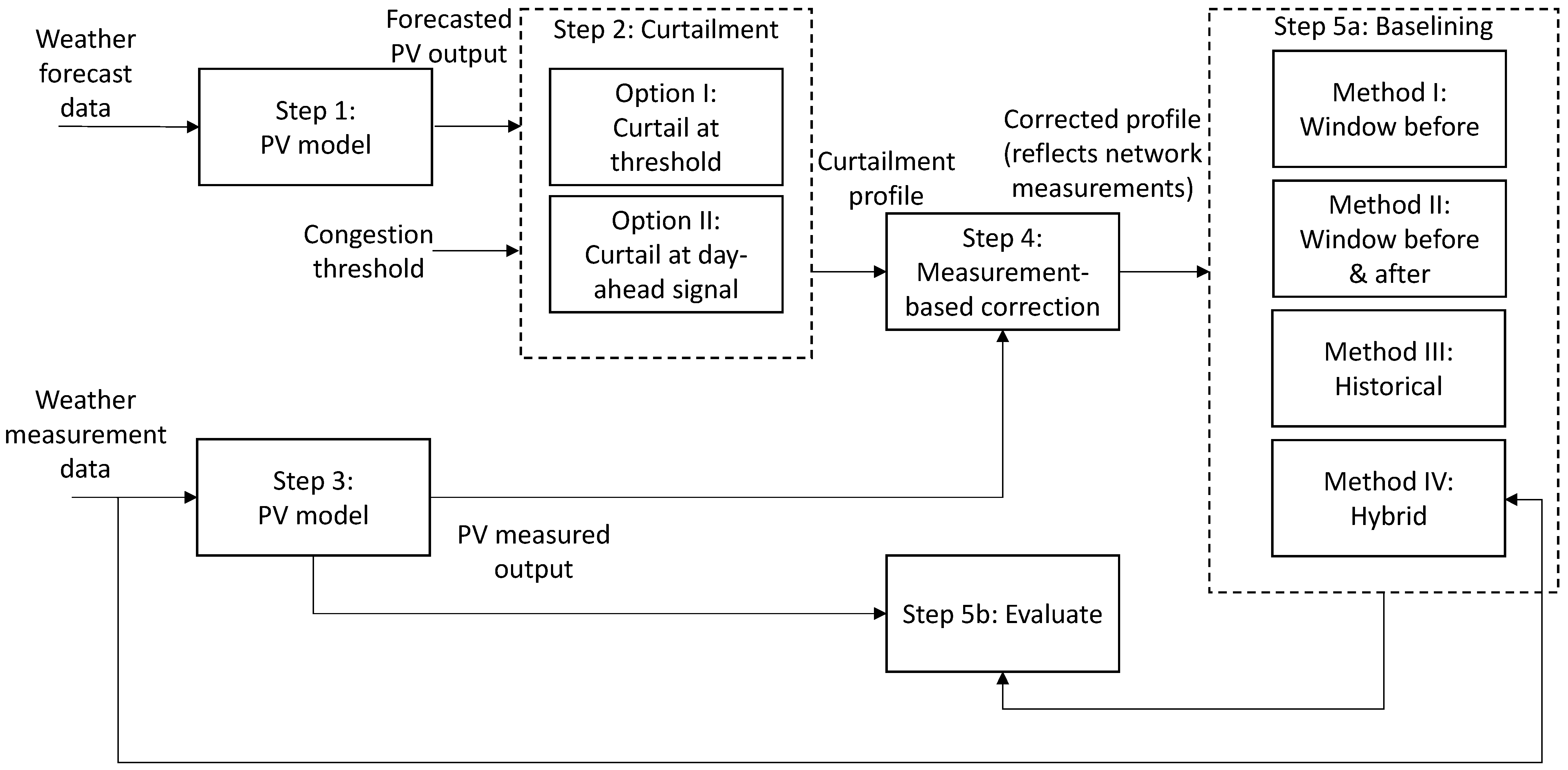
In order to evaluate the different baselining methodologies, a number of steps need to be taken. These steps follow the flowchart presented in Figure 2. The steps are briefly described below, after which a more elaborate description is provided on the implementation of the curtailment process and of the different baselining methodologies.

Step 1:

The expected day-ahead PV output is determined, using weather forecasts and the PV model described in Section 3.4.

Step 2:

The PV output profile is compared to a pre-set congestion threshold to determine the required flexibility (curtailment), and its duration.

Step 3:

The actual PV output profile is generated, using weather measurements and the PV model described in Section 3.4.

Step 4:

The actual PV output profile is cross-referenced with the expected curtailment profile, correcting the curtailment profile for the actual behaviour on the day of flexibility delivery. The output of this ex-post measurement-based correction consists of synthesised measurement profiles of the flexibility asset. In a real-life implementation this step can be skipped.

Step 5:

The various baselines are determined (a) and evaluated (b), using the root mean square error (RMSE, Equation (1)) and mean absolute error (MAE, Equation (2)) as error metrics, where $y_j$ is the reference profile and ${\widehat{y}}_j$ the baseline profile.

$$RMSE=\sqrt{\frac{1}{n}\sum _{j=1}^n{\left(y_j-{\widehat{y}}_j\right)}^2}$$

(1)

$$MAE=\frac{1}{n}\sum _{j=1}^n\left|y_j-{\widehat{y}}_j\right|$$

(2)

3.5.1. Curtailment

The (expected) curtailment profile is determined day-ahead and three variations are implemented: option 1, option 2a, and option 2b. Option 1 assumes the DSO will notify a market party that curtailment is needed during every timestep in which a predetermined congestion threshold would be (partially) exceeded. This could for example be used to facilitate larger amounts of PV in a congested region by curtailing the PV during the limited periods of time it runs at peak production. For option 2 (both a and b) it is assumed that the DSO will provide a selected curtailment window. This is for example applicable if, during some periods of time, sufficient load is present, thus curtailment of the PV installation is not necessary for a whole afternoon, but for a window of a few timesteps only, implying the DSO does not need to obtain flexibility for every peak. Option 2 is split in 2a and 2b. For option 2a no flexibility has been activated in the previous week and for option 2b flexibility has been activated in the previous week. This differentiation is of importance for baselining methods using historical data, as this historical data includes the previously activated flexibility, thus yielding a method vulnerable to the user dilemma, described in Section 2.1.5.

3.5.2. Ex-Post Measurement Based Correction

The objective of this step is synthesising a measurement profile. In a real-life implementation, this step would therefore not be required. As the curtailment profile is determined day-ahead, based on the expected PV output, a correction needs to be made to determine the actual profile as it would be measured in a real-life situation. To this end, an ex-post measurement based correction is made by comparing the PV output based on the weather measurements with the curtailment profile. When the PV production is lower than the curtailment profile, the curtailment profile is corrected downwards. When the PV production exceeds the expectation, this surplus is added to the curtailment profile. This new, corrected profile represents load measurements that would have been acquired at the flexibility asset in a real-life situation.

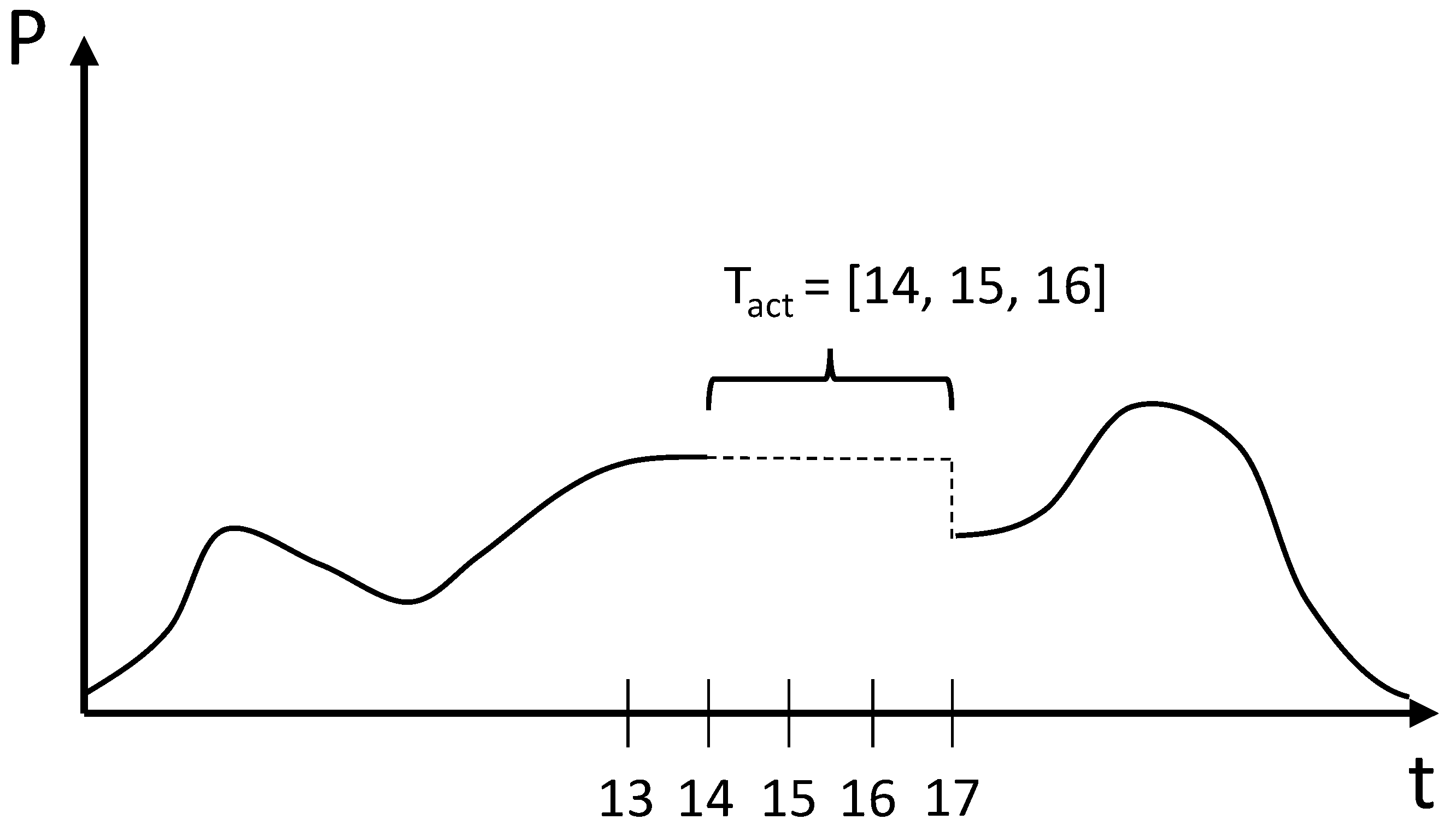
3.5.3. Baseline Method I: Window before

The window before baselining methodology is implemented by using the last measurement before flexibility activation as a baseline for the flexibility activation period. Equation (3) describes the baselining procedure mathematically, in which t is the timestep, $T_{act}$ is the list of activated timesteps, and $P_t^{meas}$ the power measurement at timestep t.

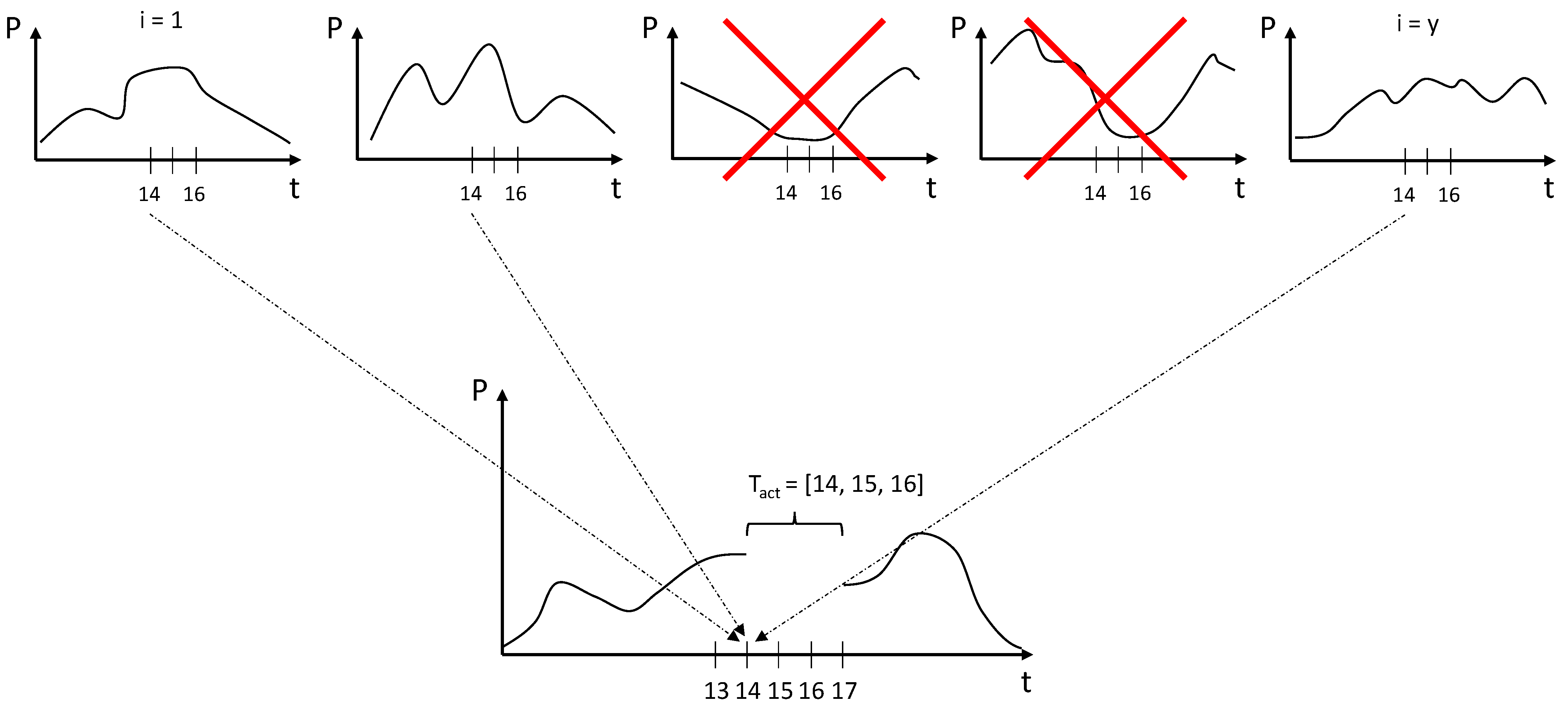
This method is illustrated in Figure 3 and the following example: Assume a curtailment request starting at 14:00 and lasting three hours. In this example, the $T_{act}=[14, 15, 16]$, and during this period the baseline is set equal to the previous timestep (in this example, timestep 13).

$${P_t}^{base}=\left\{\begin{array}{ccc}{P}_{t-1}^{meas}\hfill & if& t\in T_{act}\\ {P_t}^{meas}\hfill & otherwise& \end{array}\right.$$

(3)

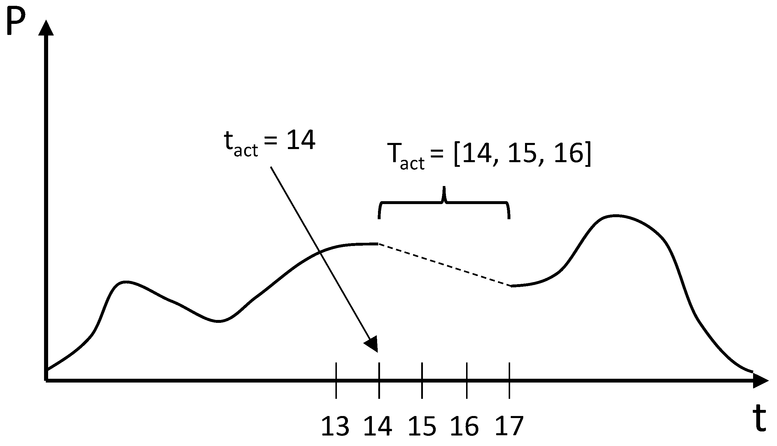
3.5.4. Baseline Method II: Window before and after

The window before and after baseline uses the last measurement before and the first measurement after the flexibility activation. During the flexibility activation, linear interpolation is used to generate a baseline for the intermediate timesteps. Equations (4) and (5) describe the baselining procedure mathematically, in which t is the timestep, $T_{act}$ is the list of activated timesteps, $\left|T_{act}\right|$ the length of the activation period, $t_{act}$ the first activated timestep, $P_t^{meas}$ the power measurement at timestep t, and $P_{t_{act}-1}^{meas}$ the power measurement at timestep $t_{act}-1$.

The method is illustrated with the same example as in Section 3.5.3. Figure 4 visualises the baseline applied for method II, illustrating the newly introduced variable $t_{act}$ (the first activated timestep, in this example 14). In this example, the baseline values for the timesteps in $T_{act}$ are derived from a linear interpolation between the last step before (timestep $t_{act}-1=13$) and first step after activation (timestep $t_{act}+\left|T_{act}\right|=17$).

$$\frac{\Delta P^{base}}{\Delta t}=\frac{P_{t_{act}+\left|T_{act}\right|}^{meas}-P_{t_{act}-1}^{meas}}{\left|T_{act}\right|+1}$$

(4)

$${P_t}^{base}=\left\{\begin{array}{ccc}\frac{\Delta P^{base}}{\Delta t}\left(t-\left(t_{act}-1\right)\right)+P_{t_{act}-1}^{meas}\hfill & if& t\in T_{act}\\ {P_t}^{meas}\hfill & otherwise& \end{array}\right.$$

(5)

3.5.5. Baseline Method III: Historical

The highest x out of y (historical) baseline is implemented using the highest 3 out of 5 historical days. As the flexibility source is PV, no differentiation is made between week days and weekend days. For each individual timestep, the same timestep is taken from the last five days, after which the three highest values obtained are averaged and used as the baseline value for the respective timestep.

Equations (6) and (7) describe the baselining procedure, where x and y represent the highest x (i.e., 3) out of y (i.e., 5), $T_{act}$ represents the list of activated timesteps, and ${\overline{P}}_t$ represents the average power at timestep t. Figure 5 illustrates this method, in which the highest 3 out of 5 historical days are used.

$$\begin{array}{ccc}\overline{P_t}=\frac{1}{x}{\displaystyle \sum _{k=0}^x}{max}_k\left(P_{i,m}\right)& \forall i,1,...,y& \forall m\end{array}\in T_{act}$$

(6)

$$P_t^{base}=\left\{\begin{array}{ccc}\overline{P_t}\hfill & if& t\in T_{act}\\ {P_t}^{meas}\hfill & otherwise& \end{array}\right.$$

(7)

3.5.6. Baseline Method IV: Combined Historical and Calculated

The authors propose a fourth, novel method. This method is a hybrid form and combines a highest x out of y (historical) baseline with a calculated correction based on the solar irradiance at the time. The highest x out of y baseline is implemented similar to baseline method III, taking the highest 3 out of 5 historical days. In addition, for each timestep, the historical measurements of the irradiance are captured. The average irradiance, corresponding with the highest 3 out of 5 measurements is then used to scale the baseline with the measurement at the timestep of activation.

Equations (8) and (9) describe the baselining procedure, where x and y represent the highest x (i.e., 3) out of y (i.e., 5), $T_{act}$ represents the list of activated timesteps, $T_{max}$ is the list of timesteps (day, hour) of the highest x out of y days, $I_t$ the irradiance at timestep t, ${\overline{I}}_t$ the average irradiance at timestep t, and the average power ${\overline{P}}_t$ is determined using Equation (6). Figure 6 illustrates this method.

$$\begin{array}{ccc}\overline{I_t}=\frac{1}{x}{\displaystyle \sum _{k=0}^x}{I}_{k,jl}& \left(j,l\right)\in T_{max}& \end{array}$$

(8)

$${P_t}^{base}=\left\{\begin{array}{ccc}\frac{I_t{\overline{P}}_t}{\overline{I_t}}\hfill & if& t\in T_{act}\\ {P_t}^{meas}\hfill & otherwise& \end{array}\right.$$

(9)

4. Results

This section presents the obtained results. First, the weather data is presented, as this has a strong influence on the further outcomes. Then, the reference profiles for the PV generation are presented. These are the profiles with which the baselines are benchmarked. This is followed by the curtailment profiles, both before and after correction. Finally, the behaviour of the baselining methods and a discussion of the results are presented.

4.1. Weather Profiles

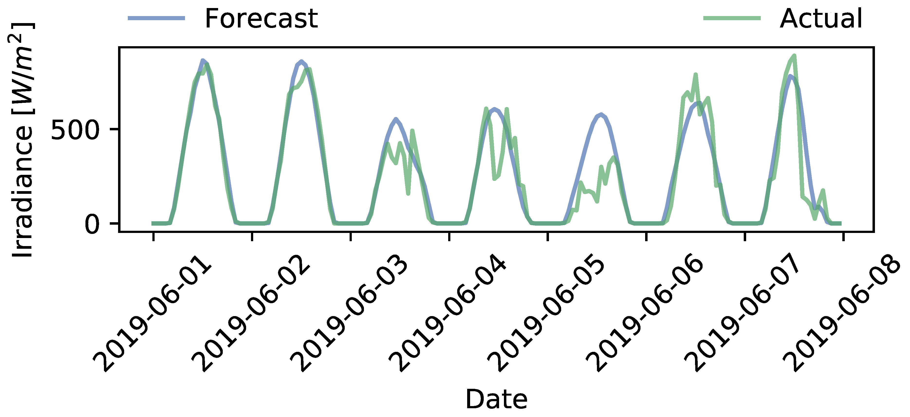
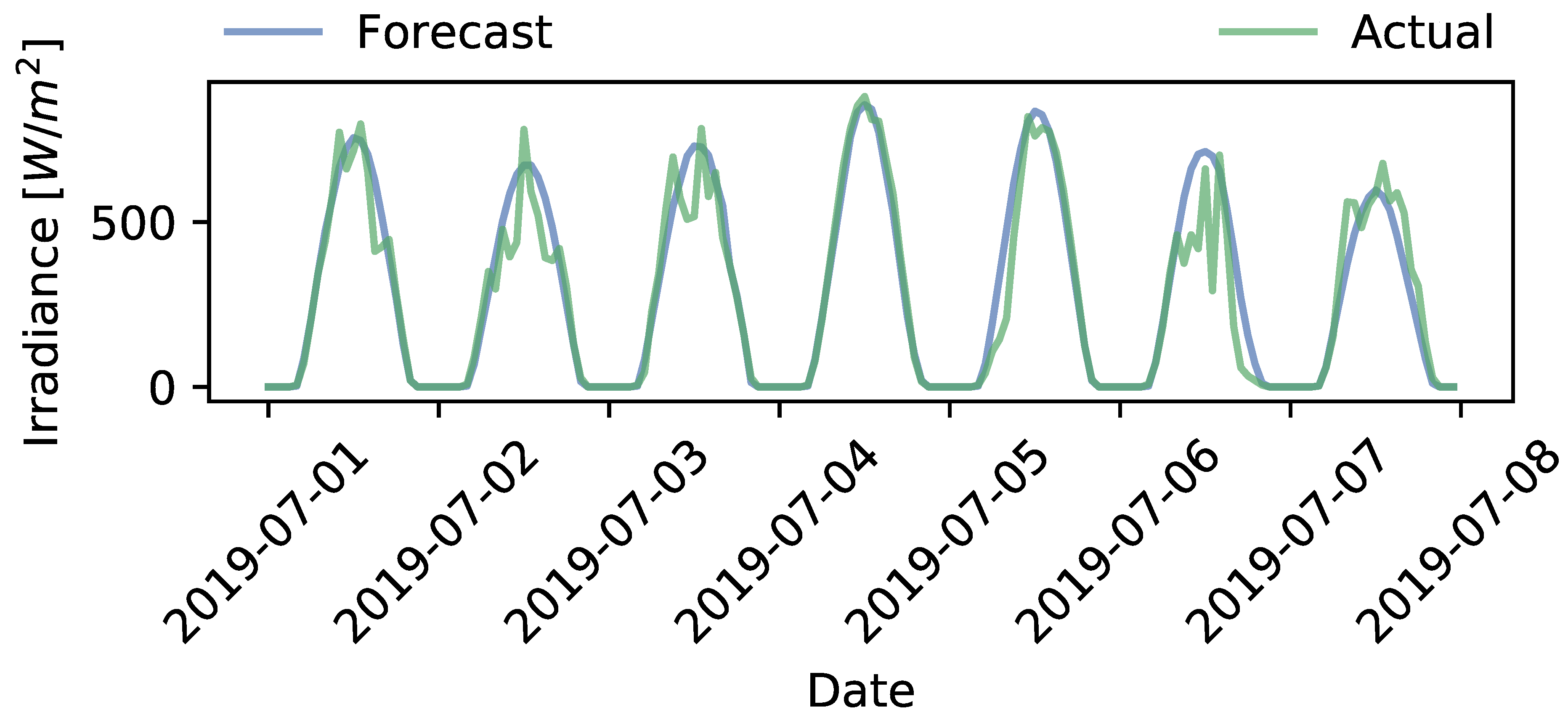
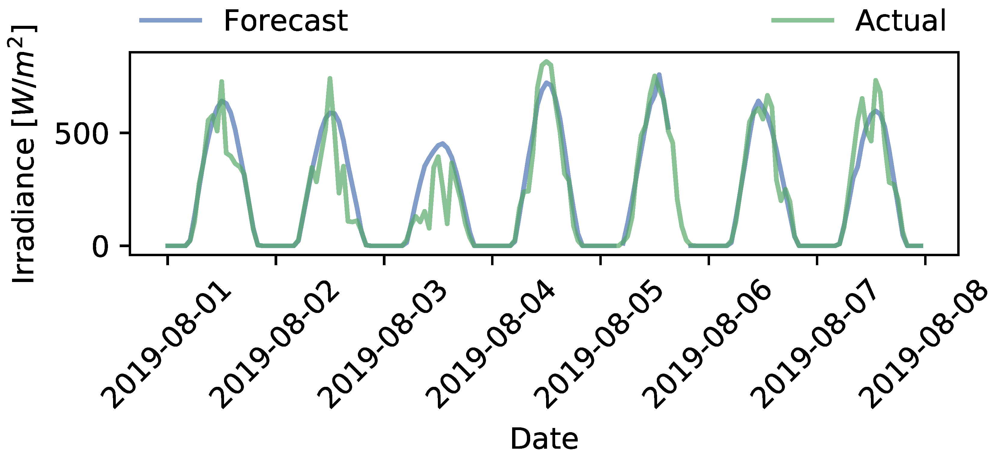
To evaluate the four baseline methods, three summer weeks with different weather profiles are selected (this research limits itself to summer weeks, as in the Netherlands curtailment of PV is not expected to occur in the winter-periods): the first week of June, July, and August. These data are used as the input for steps 1 and 3 of Section 3.5. Figure 7, Figure 8 and Figure 9 provide a visualisation of the irradiance data. It can be observed that, in terms of irradiance, the actual values differ quite a bit from the forecast. This is most likely caused by cloud movements, which are challenging to forecast accurately in a day-ahead setting. It furthermore is clear that the daily fluctuations in irradiance can be significant. This is in particular the case for the first weeks of June and August. It can be expected that this affects the results, in particular for method III, which takes historical data into account. As flexibility is expected to be needed primarily in the weeks with the highest PV production, the visualisations of the results in this section are based on the first week of July.

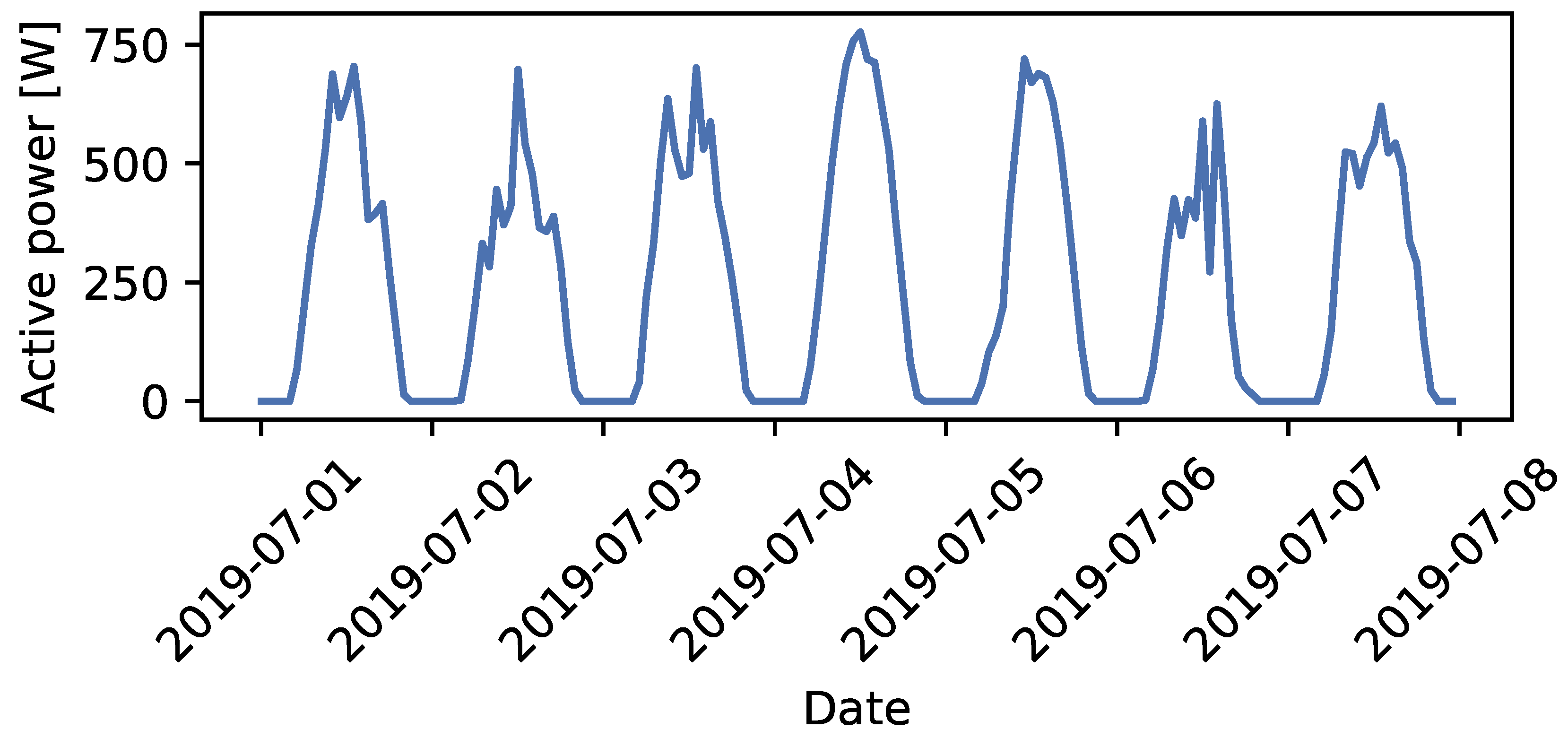
4.2. Reference Profile

The reference profile is the PV output profile generated during step 3, using irradiance measurements (Section 3.5). The reference profile reflects the unconstrained PV output, given the weather conditions. This profile is used to benchmark the performance of the selected baselining methods. The four baselining methods’ error metrics are computed using the reference profile. Figure 10 shows an example of the profile, during the first week of July 2019.

Besides benchmarking the performance of the four baselining methods, the reference profile is also used to correct the (expected, day-ahead) curtailment profiles (step 4).

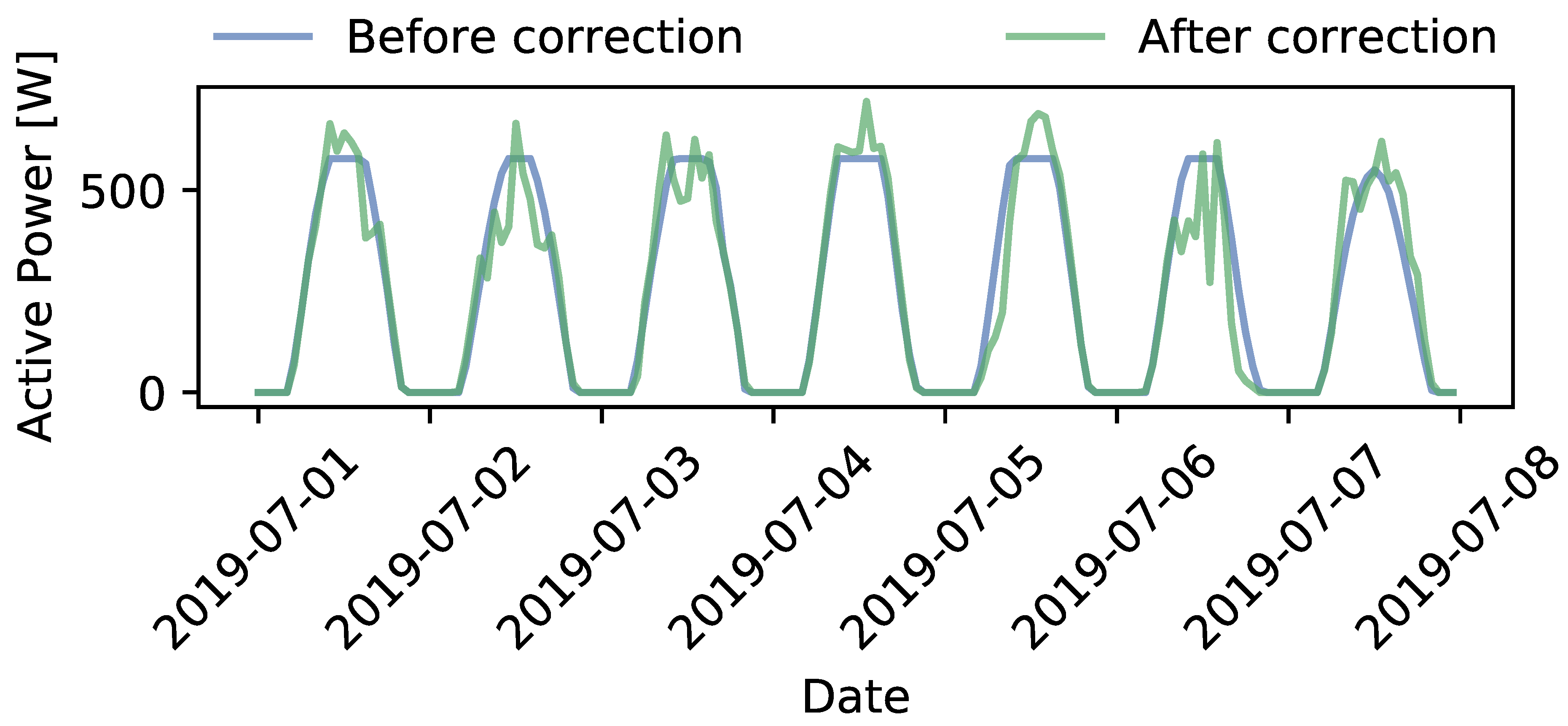
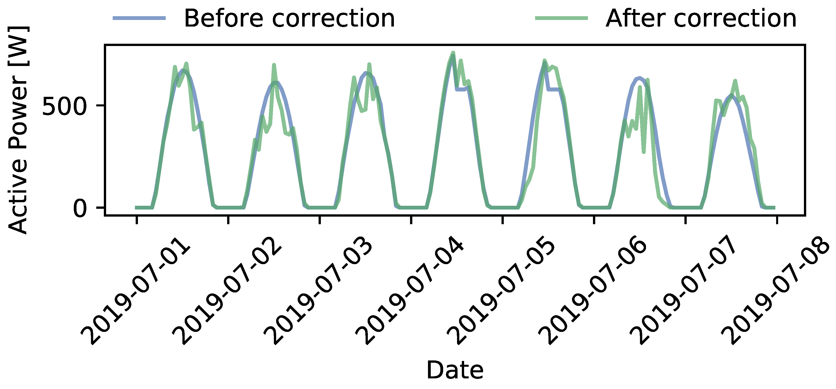
4.3. Curtailment Profiles

This research distinguishes between different curtailment variations: option 1, option 2a and option 2b (see Section 3.5.1). The day-ahead flexibility requests set a fixed curtailment level at 578 W. This value represents 75% of the maximum forecasted PV power. In case of curtailment option 1, all expected PV production larger than this limit is curtailed.

Curtailment option 2 (a and b) represents the DSO explicitly requesting flexibility at specific timeslots. In the context of this paper, this is done by manually setting curtailment limits at these timeslots. The limit is again 578 W. For option 2 (a and b) the timeslots at which curtailment is requested are the following:

• 2 June from 11:00 until 15:00
• 7 June from 10:00 until 14:00
• 4 July from 12:00 until 15:00
• 5 July from 12:00 until 16:00
• 5 August from 12:00 until 14:00

In case of curtailment option 2a, no flexibility has been enabled in the last week of May, June and July. The historical data used with methods III and IV is therefore not influenced by flexibility activation. The user dilemma (Section 2.1.5), part of the criterion proneness to manipulation, does therefore not play a significant role.

In case of option 2b, flexibility has been utilised in some of the days in the last weeks of May, June and July. This is expected to reflect back in the results of methods III and IV, as the historical data used to get the baselines is now influenced by previously activated flexibility. The additional timeslots at which flexibility is activated for curtailment option 2b are the following:

• 27 May from 12:00 until 14:00
• 29 May from 12:00 until 16:00
• 31 May from 12:00 until 14:00
• 29 June from 12:00 until 16:00
• 30 June from 12:00 until 16:00
• 1 July from 12:00 until 16:00
• 30 July from 12:00 until 14:00

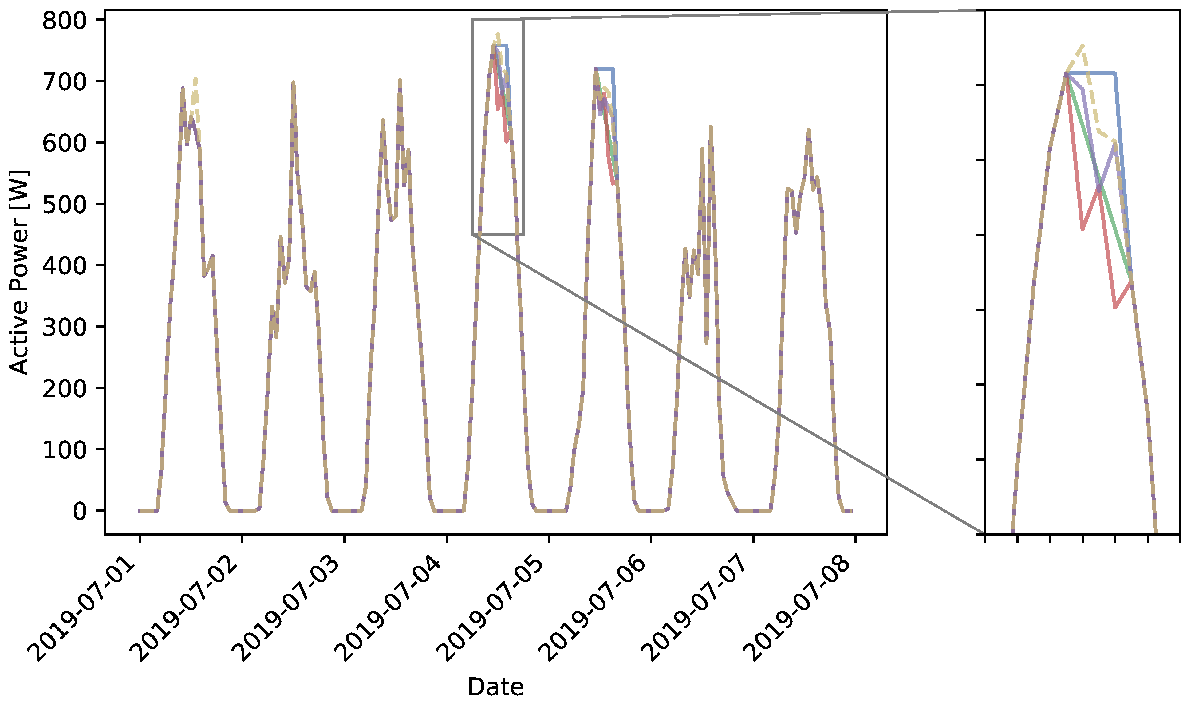
Figure 11 and Figure 12 show the curtailment profiles for curtailment options 1 and 2 (a and b). These profiles correspond with the results of steps 2 (before correction) and 4 (after correction), described in Section 3.5. It can be observed that in some cases the curtailment limit is exceeded because irradiance was higher than predicted day-ahead. Depending on how conservative a DSO sets its flexibility needs in advance, higher than expected irradiance might cause overloading as this was not foreseen when determining the (day-ahead) curtailment limit. On the other hand, it can also be observed that in some cases the day-ahead predictions overestimate the reality. This can lead to a curtailment profile, where the DSO requests market parties to provide flexibility, which, however, turns out to be no longer necessary, as in reality solar irradiance is lower than predicted.

4.4. Baselining Methods

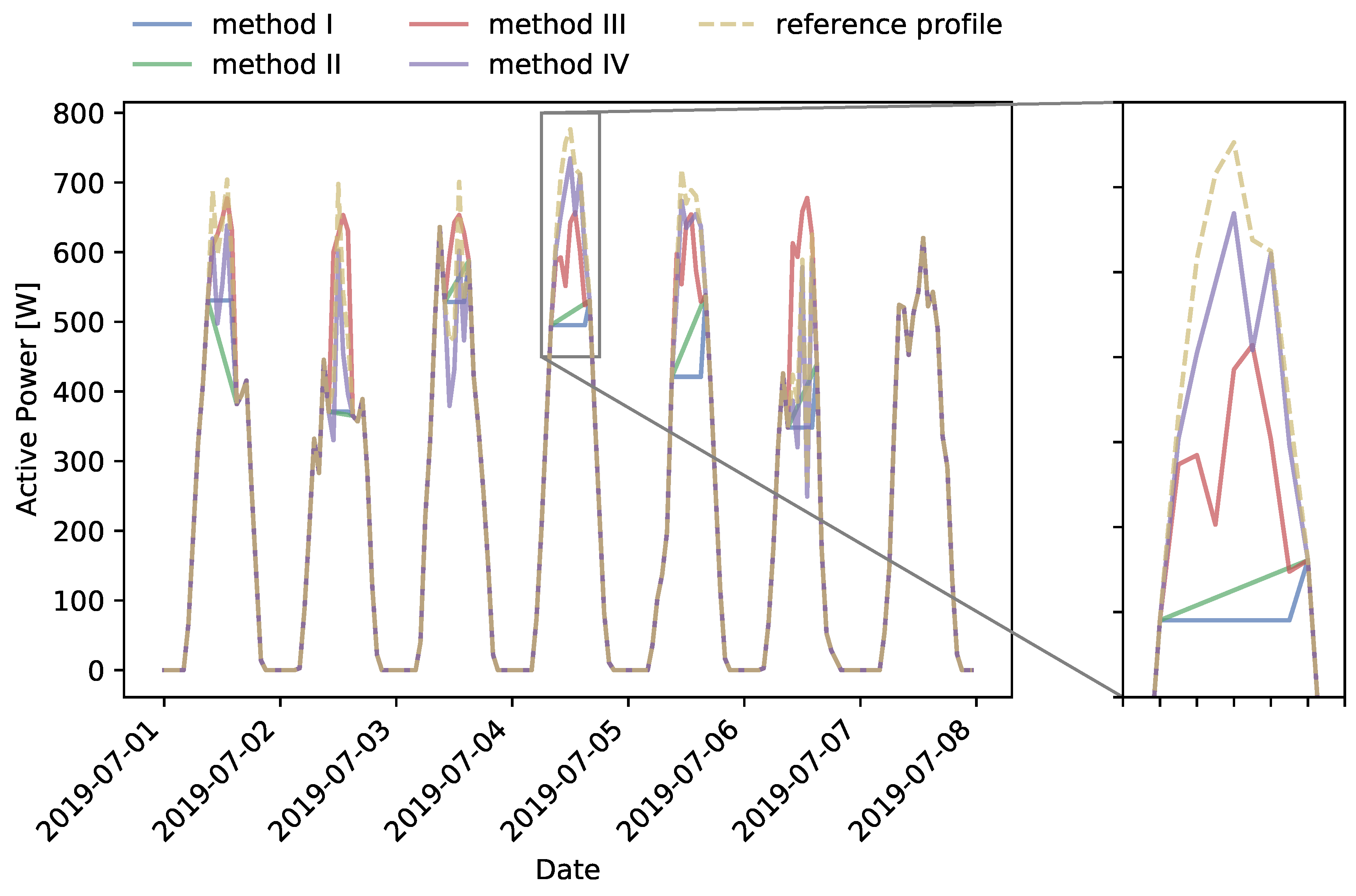
In step 5, described in Section 3.5, the baselining methods are evaluated. This is done for the curtailment options 1, 2a and 2b, and for the three first weeks of June, July and August 2019. Figure 13, Figure 14 and Figure 15 present an overview of the results for each of the four baselining methods for the different curtailment options during the first week of July 2019. This week represents a typical high PV production, during which a DSO might be expecting congestion problems.

4.4.1. Method I

Method I is the most simple way of implementing a baseline. The last measured value before flexibility activation is used as the baseline for the duration of the flexibility activation. In particular with curtailment option 1 (Figure 13), this causes significant levels of inaccuracy: when curtailing the entire peak production, method I per definition underestimates the baseline. Therefore, this baselining method is less suitable for situations in which peak PV production is continuously curtailed. In case the DSO requests flexibility from the market (curtailment option 2), this baseline’s accuracy will largely depend on the moment the DSO starts with flexibility activation, and its duration. It can be observed in Figure 14 and Figure 15 that when curtailment occurs on the peak of the day (e.g., 4 July), the baseline is an overestimate of the reference profile. Vice-versa, when curtailment starts before the peak, like in curtailment option 1 the baseline is expected to be underestimated. For flexibility activation over multiple timesteps, method I is also inaccurate. Due to the method’s simplicity, it might however perform satisfactorily for flexibility activation during a single (short) timestep, as the error will be limited.

4.4.2. Method II

Method II is based on a linearisation, using the last measured value before flexibility activation and the first measured value after flexibility activation. Like method I, method II is inaccurate when curtailing the entire afternoon PV peak. This can be observed clearly in Figure 13. For such curtailment profiles, baselining method II is therefore suitable.

When applying curtailment option 2 (a and b), method II tends to underestimate the reference profile, as can be observed in Figure 14 and Figure 15. This is inherent to the applied linearisation, in particular for smooth PV curves. Only in very specific weather conditions, with large fluctuations of PV output, method II might overestimate the reference profile. The performance of method II for curtailment option 2 (a and b) is better than for curtailment option 1. However, looking at the error metrics (

Table 3. Error metric for baselines in the first weeks of June, July and August, 2019. Units in [W].

	Option 1		Option 2a		Option 2b
	MAE	RMSE	MAE	RMSE	MAE	RMSE
1–8 June
Method I	9.00	31.44	3.47	18.78	3.47	18.78
Method II	15.87	60.75	8.80	52.65	8.80	52.65
Method III	12.31	44.86	5.27	29.84	5.64	30.45
Method IV	3.12	11.47	0.98	5.19	1.07	5.74
1–8 July
Method I	30.19	80.34	1.86	10.05	2.37	12.03
Method II	29.27	75.44	1.92	10.07	2.43	12.04
Method III	19.22	56.71	2.45	14.83	3.49	18.45
Method IV	10.01	26.38	0.45	2.63	1.41	8.28
1–8 August
Method I	7.61	40.53	4.71	36.14	4.71	36.14
Method II	9.37	45.37	4.85	36.28	4.85	36.28
Method III	8.54	43.29	4.34	35.78	4.34	35.78
Method IV	5.10	36.04	4.27	35.77	4.27	35.77

), overall baselining method I outperforms baselining method II.

4.4.3. Method III

Method III takes into account the last five days and uses the measurements of the three with the highest production. Looking at Figure 13, this method seems to be approximating the reference profile relatively well in the first few days of the week. On the 4th of July, it can be observed that, due to the relatively low profiles of the past days, method III underestimates the reference profile.

Looking at curtailment option 2, method III is relatively sensitive to previous flexibility activation, as this influences the historical data used to construct the baseline. This can be observed clearly by comparing Figure 14 with Figure 15. Looking at the zoom-box of the fourth of July, the profile of baselining method III is changed significantly in the latter figure.

4.4.4. Method IV

The new method IV, proposed by the authors, combines the historical data used in method III, with historical and actual irradiance measurements. As a result, the baseline is better able to follow the pattern of the reference profile. However, from Figure 13, it can be observed that this is typically with a downward bias in case curtailment option 1 is applied. Compared with methods I, II and III, our new method shows an improvement in accuracy for all curtailment options. For curtailment option 2a and 2b, the profile has the highest accuracy, with a mean absolute error of maximum 4.27 W in the first week of August. Furthermore, the historical flexibility activations introduced in curtailment option 2b have less impact on the outcome of method IV compared to method III.

4.5. Error Metric

For each of the three evaluated weeks, the mean absolute error (MAE) and root mean square error (RMSE) are determined (see Section 3.5). The results are presented in Table 3. For an additional three weeks, the error metrics can be found in Appendix A.

Comparing methods II and III, method III in general performs better. This method is based on the historical data, which can result in situations in which the opposite holds and the accuracy of method III is lower than the accuracy of method II. This is in particular the case for the first week of July, using curtailment option 2. Figure 14 shows that the first few days of July have a lower PV output. As these days are used to generate the baseline, this directly influences the result. In case of curtailment option 2b, this effect is increased due to flexibility activations being incorporated in the historical dataset.

It can be observed that overall, the performance of the new baselining method IV is better than that of methods I, II and III. Furthermore, the impact of the user dilemma on methods III and IV can be observed in curtailment option 2b. For these two methods, the error increases slightly when flexibility activation has occurred in the measurements of the historical days used to generate the baselines. This was to be expected, but the effect is relatively small, especially for method IV.

Overall it can be observed that the accuracy in weeks with volatile PV irradiance, like the first week of August, is significantly lower. This is because the historical data on which some of the baselines are based are strongly affected by this volatility. For curtailment option 1, the accuracy seems to decrease less during volatile weather, which can be explained by the lower amounts of flexibility activation.

The accuracy’s dependency on the actual weather situation shows one of the trade-offs a DSO must be prepared to make. When implementing baselining methods that are simple and transparent, there situations during which the performance of those baselines is lower are inevitable. This is not necessarily problematic, as the expectation is that the majority of flexibility activations will be during peak PV production weeks. Should a DSO often need flexibility in weeks with volatile PV output, alternative, more complex baselining methods might be required.

4.6. Discussion

The presented accuracy comparisons and error metrics are dependent on the used weather data, number and duration of flexibility requests and the magnitude of the curtailment. For a proof-of-concept of a newly developed transparent and simple method proposed in this paper, three summer weeks with different profiles have been selected. Each week gives a different result, which is to be expected when weeks with different profiles are compared. In particular weeks with a highly volatile irradiance profile have a large impact on the error metric (i.e., result in a worse performance). The error metrics of three additional weeks are presented in Appendix A. In future work, a broader statistical analysis is needed to ensure the results are valid in general.

As the baseline is equal to the measurement when no flexibility is activated, the amount and duration of flexibility requests also influences the baselining error. Increasing the number and/or duration of activations will increase the error of the baseline, as for those periods the baseline is no longer equal to the measurement (thus the error is no longer zero).

The error metrics should therefore not be interpreted in absolute sense. The MAE and RMSE provide a way to compare the four baselining methods, under the specific circumstances they have been tested for. This gives insight in their accuracy in similar situations. However, to get a better view, a simulation over a longer period of time would be required, including a platform to generate market-based flexibility activations. This is a topic for future research.

When implementing a simulation over a longer period of time, including a platform to generate flexibility activations or requests, the availability of flexibility can also be taken into account. For this paper, it is assumed that when flexibility is requested by the DSO, the market will offer it and the flexibility is indeed available at the moment of delivery. However, in a real-life situation not every flexibility request may be fulfilled and not all promised flexibility will be delivered. The resulting uncertainty affects the baselines, as the historical measurements depend on the activation (no delivered flexibility means no user dilemma). This again impacts the performance.

For method IV, the baseline is scaled using weather data. As the DSO does not necessarily have the same weather dataset as market parties have, it is important to evaluate the impact of using different datasets for the applied scaling, including using weather data from different locations, which is likely to happen given the limited amount of weather stations in relation to the spread of PV systems. To explore this we have used a weather dataset from the other side of the city. As the difference in output for baselining method IV was <2.5 W, or <1%, in our case the impact is negligible, but this topic also needs to be investigated further.

Our new method IV introduces an improvement compared to baselining methods I, II and III, while keeping the method as simple and transparent as possible. However, the accuracy improvement depends on the weather, and during periods with highly volatile irradiance profiles, the error may be higher. In case this is not acceptable, and a DSO is willing to compromise on the simplicity and transparency criteria, alternative methods might be considered (e.g., methods in the calculated or machine learning domain, see Section 2.2). Alternatively, the DSO might implement a prognosis-based baseline. For this paper, we have not considered this method, as the nature of the problem of determining a baseline is not solved by shifting this responsibility from the DSO to a market party (e.g., aggregator).

This paper focuses on a baselining method that can be used in combination with PV systems. Due to the strong dependency on a single parameter (i.e., irradiance), we expect this method might also apply to other flexibility sources that have a similar, single parameter, dependency (e.g., heat pumps, cooling installations). This assumption is a topic for further research.

5. Conclusions

This paper has evaluated four methods to establish a baseline when flexibility is provided by PV systems. The methods are selected for their simplicity and transparency, two key criteria in order for DSOs and market parties to accept and implement a baselining method. This is done for different curtailment strategies: downward curtailment towards a certain threshold value and day-ahead flexibility requests.

It is shown in this paper that three existing methods have shortcomings in terms of accuracy, in particular when curtailing downward to a threshold value. A proof-of-concept is provided for a fourth method, developed by the authors. It is shown that this method, while maintaining simplicity and transparency, performs better for the cases investigated in this paper. In cases of high PV production and a relatively smooth irradiance profile, this method is preferable. The extent of improvement is however dependent on the volatility of the irradiance profile.

Future work consists of two main elements. First, the current research evaluates baselines based on three independent weeks with a limited set of flexibility activations. Future research considering longer periods of time and including more frequent flexibility activations is required to further explore the performance improvement brought by the new method. Second, the current methods are evaluated for PV systems only. Future work should evaluate whether other flexibility assets, in particular those with a strong dependency on a single parameter can be described by this method as well.