Modified Crack Detection of Sewer Conduit with Low-Resolution Images

Abstract

Imaging devices of less than 300,000 pixels are mostly used for sewage conduit exploration due to the petty nature of the survey industry in Korea. Particularly, devices of less than 100,000 pixels are still widely used, and the environment for image processing is very dim. Since the sewage conduit images covered in this study have a very low resolution (240 × 320 = 76,800 pixels), it is very difficult to detect cracks. Because most of the resolutions of the sewer conduit images are very low in Korea, this problem of low resolution was selected as the subject of this study. Cracks were detected through a total of six steps of improving the crack in Step 2, finding the optimal threshold value in Step 3, and applying an algorithm to detect cracks in Step 5. Cracks were effectively detected by the optimal parameters in Steps 2 and 3 and the user algorithm in Step 5. Despite the very low resolution, the cracked images showed a 96.4% accuracy of detection, and the non-cracked images showed 94.5% accuracy. Moreover, the analysis was excellent in quality. It is believed that the findings of this study can be effectively used for crack detection with low-resolution images.

1. Introduction

The recent urban sinkholes in Korea are often caused by the loss of surrounding soil due to the aging of a sewer built intensively in the 1970s and 1980s. In the case of Korea, 980 local governments nationwide have conducted a detailed investigation of 12,000 km of the entire sewer, which is over 20 years old, to prevent sinkholes.

Since the current structure maintenance technique evaluates the condition with the naked eye of the inspector based on manpower, a lot of time and effort is consumed, resulting in the poor objectivity and reliability of the survey. One of the ways to compensate for this problem is to use digital image processing technology.

Recently, studies on the introduction of an image processing technique capable of analyzing the CCTV images of a sewer or the development of the devices are being conducted. Xu et al. [1] measured the deformation of the sewer through image analysis using a probe equipped with an annular laser pointer. McKim et al. [2] extracted information on cracks in a sewer using basic image processing techniques, and Moselhi et al. [3] applied artificial neural network method complementarily. Later, Yang and Su [4] studied an advanced image processing method of applying machine learning, and Yang et al. [5] also proposed a method for evaluating the quality of images taken from the sewer. Sinha et al. [6] studied the automated detection of cracks in buried concrete pipe images, and Halfawy et al. [7] tested the proposed algorithm on a set of CCTV videos obtained from the cities of Regina and Calgary in Canada. Recently, Haurum et al. [8] analyzed papers on CCTV sewer survey images. However, there is a limit to the application of the developed image processing method, because the quality of the image taken while navigating in such a dark environment with a lot of obstacles as the sewer is very low.

As for the sewer exploration device, a high-resolution digital camera of more than 2 million pixels has been developed. However, devices of less than 300,000 pixels are mostly being used in Korea because of the small size of the Korean survey industry and the low awareness of the severity of the sewer problem in Korea.

The sewer conduit images covered in this study are of 76,800 pixels (240 × 320), and it is difficult to detect cracks at such low resolution. Son et al. [9,10] studied the crack detection method of these low-resolution sewer images twice in 2017 [9] and 2019 [10]. Their 2019 [8] study showed relatively high accuracy research results, but it is a bit complicated to apply. An investigation improving crack detection to compensate for these problems was conducted in this study.

2. Crack Detection Procedure

As shown in

Table 1. Specification of sewer video clip.

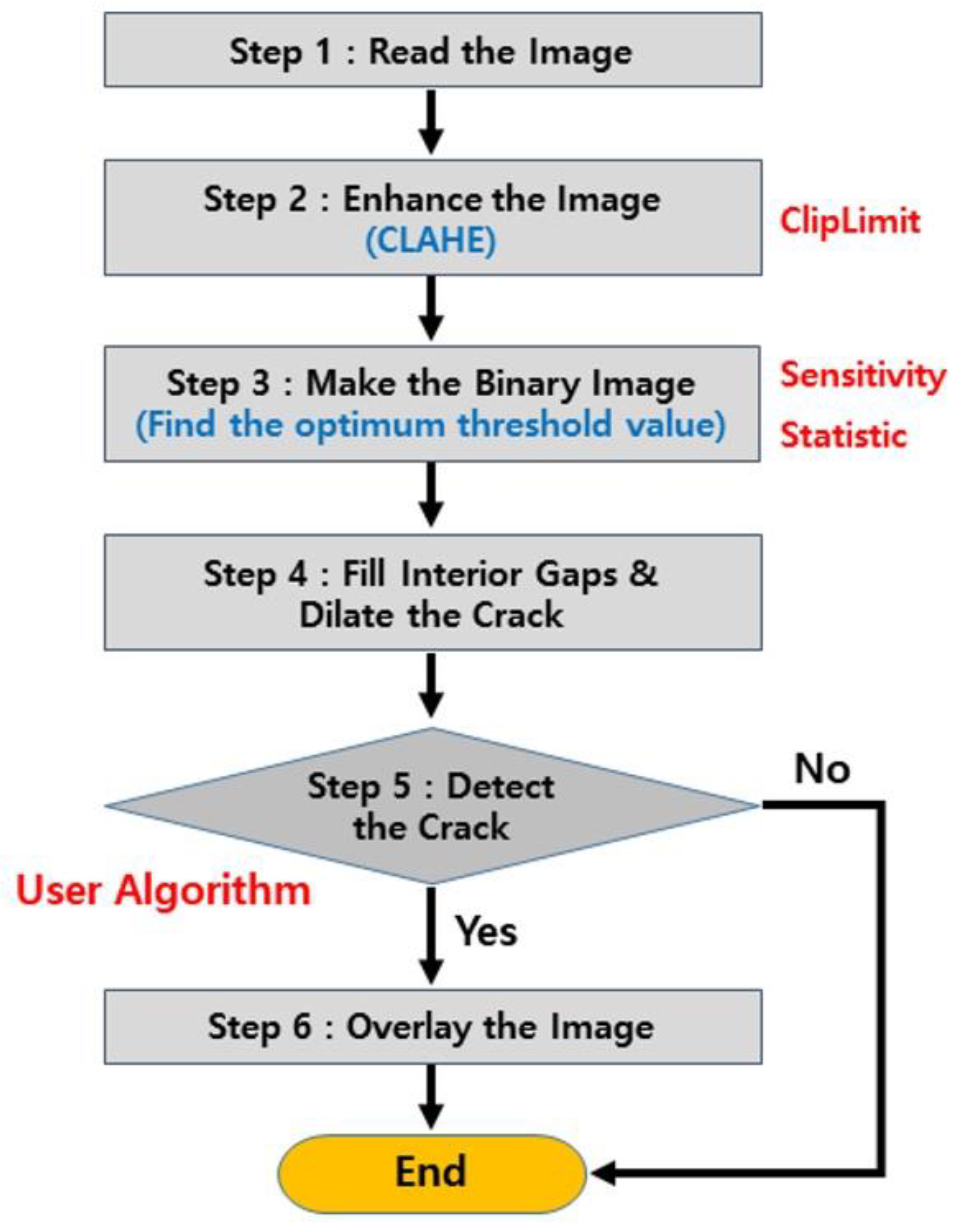
Duration	200 s
Frame Rate	30
Height	240
Width	320

, the sewer CCTV image is a video clip of 200 s in duration in very low-resolution images of 76,800 pixels (240 × 320). A total of 110 images were selected as analysis targets, excluding unnecessary (such as the beginning of the video clip) and overlapping images from a total of 200 images of one image per second. Of the 110 images, both cracked images (c1~c55) and non-cracked images (n1~n55) counted 55 each, and 20 sample data are shown in Figure 1 and Figure 2.

The crack detection procedure for low-resolution images goes through six steps as shown in

Table 2. Crack detection procedure.

Procedures for Crack Detection	Crack Image (c18)	Non-Crack Image (n25)
Step 1 Read the Image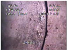
Step 2 Enhance the Image (CLAHE: Contrast-Limited Adaptive Histogram Equalization) (Parameter: ClipLimit)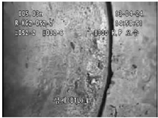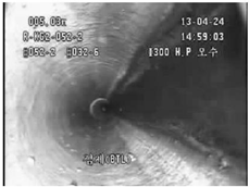
Step 3 Make the Binary Image (Find the Optimum Threshold Value) (Parameter: Sensitivity and Statistic)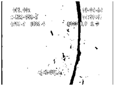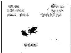
Step 4 Fill Interior Gaps and Dilate the Crack
Step 5 Detect the Crack (Complement the Image) (User Algorithm)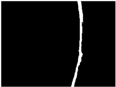
Step 6 Overlay the Image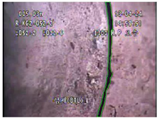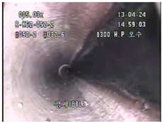

and Figure 3. The important steps in this procedure are Steps 2, 3, and 5, and the crack detection process for each step is summarized as follows.

2.1. Step 1: Read the Image

This is the stage of reading the original video of the sewer. Table 2 shows c18 and n25 as examples among 55 cracked images and 55 non-cracked images.

2.2. Step 2: Enhance the Image

First, a color image is converted into a grayscale image, and the image is enhanced in this step. There are many ways to enhance the image. This study applied the method of Contrast-Limited Adaptive Histogram Equalization (CLAHE) proposed by Zuiderveld [11]. CLAHE is a method widely used for contrast enhancement. Among the various parameters of CLAHE, an important parameter in this study is ClipLimit. The smaller the ClipLimit is, the more the histogram value redistributed from the maximum value increases, resulting in a more pronounced contrast. The range is a real number between 0 and 1, and the example in Table 2 uses 0. The parameter study of the changing ClipLimit between 0 and 1 is discussed in Section 3.

2.3. Step 3: Make the Binary Image

This step converts analog images to binary images. For crack detection, it is necessary to determine an optimal threshold value. The method proposed by Bradley [12] was used to compute it, and the parameters of step 3 were sensitivity and statistical analysis.

Sensitivity assigns a real number between 0 and 1. If the value is large, there is a risk of including some background pixels. Despite the risk, the larger pixels are regarded as a foreground for the binary conversion. Statistical methods can be selected from mean, median, or Gaussian. Mean is the local average value of the neighborhood, the median is the local median of the neighborhood, and Gaussian uses the Gaussian weighted average of the neighborhood as a statistic.

In the example of Table 2, the sensitivity was 1, and the chosen statistic was Gaussian. The parameter study of the sensitivity and statistical method is conducted in Section 3.

2.4. Step 4: Fill Interior Gaps and Dilate the Crack

This step involves filling the inside of the crack and expanding the crack. The method proposed by Soille [13] was used to fill the inside of the crack, and cracks mostly remain. Any deformation, that is not a crack, can be removed through the following step. The image dilation method proposed by Gonzalez et al. [14] was applied to highlight the cracks.

2.5. Step 5: Detect the Crack

This step determines the presence or absence of cracks, i.e., extracting only the cracks. This determines whether the object filled in the interior in Step 4 is a crack or not. In this step, a User Algorithm is required and will be explained in detail in Chapter 3. Additionally, it is a step inverting the black and the white color of the image to improve readability.

2.6. Step 6: Overlay the Image

Finally, is the step of overlaying the detected crack boundary on the original image. The method proposed by Gonzalez et al. [14] was used.

3. Crack Detection Parameters and User Algorithm

Finally, this stage overlays the detected crack boundary on the original image by the method of Gonzalez et al. [14].

3.1. Crack Detection Parameters

Table 3. Analysis parameters.

Var. #	Name	Range
Var. #1	ClipLimit	0, 0.00001, 0.0001, 0.01, [0.1:0.1:1] {15}
Var. #2	Sensitivity	[0:0.1:1] (start:spacing:end) {11}
Var. #3	Statistic	Mean, Median, Gaussian {3}

shows the analysis parameters described in Section 2, and

Table 4. Analysis results (%) by Var. #1 vs. Var. #2 (Var. #3: Mean).

(a) Crack Images
	Var. #2	0.0	0.1	0.2	0.3	0.4	0.5	0.6	0.7	0.8	0.9	1.0
Var. #1
0		0.0	0.0	0.0	0.0	0.0	3.6	87.3	92.7	96.4	94.5	94.5
0.00001		0.0	0.0	0.0	0.0	0.0	3.6	87.3	92.7	96.4	94.5	94.5
0.0001		0.0	0.0	0.0	0.0	0.0	3.6	87.3	92.7	96.4	94.5	94.5
0.001		0.0	0.0	0.0	0.0	1.8	5.5	78.2	90.9	96.4	94.5	94.5
0.01		0.0	0.0	0.0	0.0	0.0	5.5	52.7	92.7	98.2	100.0	98.2
0.1		0.0	0.0	0.0	0.0	0.0	5.5	45.5	90.9	98.2	100.0	100.0
0.2		0.0	0.0	0.0	0.0	0.0	5.5	47.3	90.9	98.2	100.0	100.0
0.3		0.0	0.0	0.0	0.0	0.0	5.5	49.1	90.9	98.2	100.0	100.0
0.4		0.0	0.0	0.0	0.0	0.0	5.5	49.1	90.9	98.2	100.0	100.0
0.5		0.0	0.0	0.0	0.0	0.0	5.5	49.1	90.9	98.2	100.0	100.0
0.6		0.0	0.0	0.0	0.0	0.0	5.5	49.1	90.9	98.2	100.0	100.0
0.7		0.0	0.0	0.0	0.0	0.0	5.5	49.1	90.9	98.2	100.0	100.0
0.8		0.0	0.0	0.0	0.0	0.0	5.5	49.1	90.9	98.2	100.0	100.0
0.9		0.0	0.0	0.0	0.0	0.0	5.5	49.1	90.9	98.2	100.0	100.0
1.0		0.0	0.0	0.0	0.0	0.0	5.5	49.1	90.9	98.2	100.0	100.0
(b) Non-Crack Images
	Var. #2	0.0	0.1	0.2	0.3	0.4	0.5	0.6	0.7	0.8	0.9	1.0
Var. #1
0		100.0	100.0	100.0	100.0	100.0	100.0	65.5	25.5	70.9	94.5	98.2
0.00001		100.0	100.0	100.0	100.0	100.0	100.0	65.5	25.5	70.9	94.5	98.2
0.0001		100.0	100.0	100.0	100.0	100.0	100.0	65.5	25.5	70.9	94.5	98.2
0.001		100.0	100.0	100.0	100.0	100.0	98.2	67.3	20.0	49.1	94.5	98.2
0.01		100.0	100.0	100.0	100.0	100.0	100.0	70.9	9.1	10.9	40.0	72.7
0.1		100.0	100.0	100.0	100.0	100.0	98.2	70.9	5.5	5.5	14.5	40.0
0.2		100.0	100.0	100.0	100.0	100.0	96.4	72.7	9.1	5.5	18.2	43.6
0.3		100.0	100.0	100.0	100.0	100.0	96.4	70.9	9.1	7.3	16.4	43.6
0.4		100.0	100.0	100.0	100.0	100.0	96.4	70.9	9.1	5.5	14.5	43.6
0.5		100.0	100.0	100.0	100.0	100.0	96.4	69.1	9.1	5.5	14.5	43.6
0.6		100.0	100.0	100.0	100.0	100.0	96.4	70.9	9.1	5.5	14.5	43.6
0.7		100.0	100.0	100.0	100.0	100.0	96.4	70.9	9.1	5.5	14.5	43.6
0.8		100.0	100.0	100.0	100.0	100.0	96.4	70.9	9.1	5.5	14.5	43.6
0.9		100.0	100.0	100.0	100.0	100.0	96.4	70.9	9.1	5.5	14.5	43.6
1.0		100.0	100.0	100.0	100.0	100.0	96.4	70.9	9.1	5.5	14.5	43.6

,

Table 5. Analysis results (%) by Var. #1 vs. Var. #2 (Var. #3: Median).

(a) Crack Images
	Var. #2	0.0	0.1	0.2	0.3	0.4	0.5	0.6	0.7	0.8	0.9	1.0
Var. #1
0		0.0	0.0	0.0	0.0	0.0	0.0	49.1	98.2	94.5	87.3	83.6
0.00001		0.0	0.0	0.0	0.0	0.0	0.0	49.1	98.2	94.5	87.3	83.6
0.0001		0.0	0.0	0.0	0.0	0.0	0.0	49.1	98.2	94.5	87.3	83.6
0.001		0.0	0.0	0.0	0.0	0.0	0.0	41.8	98.2	94.5	92.7	85.5
0.01		0.0	0.0	0.0	0.0	0.0	0.0	34.5	96.4	98.2	100.0	90.9
0.1		0.0	0.0	0.0	0.0	0.0	1.8	29.1	90.9	98.2	100.0	96.4
0.2		0.0	0.0	0.0	0.0	0.0	1.8	27.3	92.7	100.0	100.0	96.4
0.3		0.0	0.0	0.0	0.0	0.0	1.8	29.1	92.7	100.0	100.0	96.4
0.4		0.0	0.0	0.0	0.0	0.0	1.8	29.1	92.7	100.0	100.0	96.4
0.5		0.0	0.0	0.0	0.0	0.0	1.8	29.1	92.7	100.0	100.0	96.4
0.6		0.0	0.0	0.0	0.0	0.0	1.8	29.1	92.7	100.0	100.0	96.4
0.7		0.0	0.0	0.0	0.0	0.0	1.8	29.1	92.7	100.0	100.0	96.4
0.8		0.0	0.0	0.0	0.0	0.0	1.8	29.1	92.7	100.0	100.0	96.4
0.9		0.0	0.0	0.0	0.0	0.0	1.8	29.1	92.7	100.0	100.0	96.4
1.0		0.0	0.0	0.0	0.0	0.0	1.8	29.1	92.7	100.0	100.0	96.4
(b) Non-Crack Images
	Var. #2	0.0	0.1	0.2	0.3	0.4	0.5	0.6	0.7	0.8	0.9	1.0
Var. #1
0		100.0	100.0	100.0	100.0	100.0	100.0	72.7	32.7	90.9	100.0	100.0
0.00001		100.0	100.0	100.0	100.0	100.0	100.0	72.7	32.7	90.9	100.0	100.0
0.0001		100.0	100.0	100.0	100.0	100.0	100.0	72.7	32.7	90.9	100.0	100.0
0.001		100.0	100.0	100.0	100.0	100.0	100.0	61.8	21.8	80.0	100.0	100.0
0.01		100.0	100.0	100.0	100.0	100.0	100.0	69.1	1.8	20.0	54.5	85.5
0.1		100.0	100.0	100.0	100.0	100.0	100.0	72.7	3.6	7.3	18.2	40.0
0.2		100.0	100.0	100.0	100.0	100.0	100.0	72.7	3.6	3.6	18.2	41.8
0.3		100.0	100.0	100.0	100.0	100.0	100.0	70.9	3.6	0.0	18.2	41.8
0.4		100.0	100.0	100.0	100.0	100.0	100.0	70.9	3.6	0.0	18.2	41.8
0.5		100.0	100.0	100.0	100.0	100.0	100.0	72.7	3.6	0.0	18.2	41.8
0.6		100.0	100.0	100.0	100.0	100.0	100.0	72.7	3.6	0.0	18.2	41.8
0.7		100.0	100.0	100.0	100.0	100.0	100.0	72.7	3.6	0.0	18.2	41.8
0.8		100.0	100.0	100.0	100.0	100.0	100.0	72.7	3.6	0.0	18.2	41.8
0.9		100.0	100.0	100.0	100.0	100.0	100.0	72.7	3.6	0.0	18.2	41.8
1.0		100.0	100.0	100.0	100.0	100.0	100.0	72.7	3.6	0.0	18.2	41.8

and

Table 6. Analysis results (%) by Var. #1 vs. Var. #2 (Var. #3: Gaussian).

(a) Crack Images
	Var. #2	0.0	0.1	0.2	0.3	0.4	0.5	0.6	0.7	0.8	0.9	1.0
Var. #1
0		0.0	0.0	0.0	0.0	9.1	34.5	76.4	90.9	96.4	98.2	96.4
0.00001		0.0	0.0	0.0	0.0	9.1	34.5	76.4	90.9	96.4	98.2	96.4
0.0001		0.0	0.0	0.0	0.0	9.1	34.5	76.4	90.9	96.4	98.2	96.4
0.001		0.0	0.0	0.0	0.0	7.3	36.4	81.8	92.7	96.4	98.2	96.4
0.01		0.0	0.0	0.0	3.6	10.9	30.9	63.6	94.5	98.2	100.0	98.2
0.1		0.0	0.0	0.0	3.6	14.5	38.2	50.9	90.9	96.4	100.0	100.0
0.2		0.0	0.0	0.0	3.6	14.5	34.5	54.5	90.9	96.4	100.0	100.0
0.3		0.0	0.0	0.0	3.6	12.7	34.5	54.5	90.9	96.4	100.0	100.0
0.4		0.0	0.0	0.0	3.6	12.7	34.5	54.5	90.9	96.4	100.0	100.0
0.5		0.0	0.0	0.0	3.6	12.7	34.5	54.5	90.9	96.4	100.0	100.0
0.6		0.0	0.0	0.0	3.6	12.7	34.5	54.5	90.9	96.4	100.0	100.0
0.7		0.0	0.0	0.0	3.6	12.7	34.5	54.5	90.9	96.4	100.0	100.0
0.8		0.0	0.0	0.0	3.6	12.7	34.5	54.5	90.9	96.4	100.0	100.0
0.9		0.0	0.0	0.0	3.6	12.7	34.5	54.5	90.9	96.4	100.0	100.0
1.0		0.0	0.0	0.0	3.6	12.7	34.5	54.5	90.9	96.4	100.0	100.0
(b) Non-Crack Images
	Var. #2	0.0	0.1	0.2	0.3	0.4	0.5	0.6	0.7	0.8	0.9	1.0
Var. #1
0		100.0	100.0	100.0	100.0	100.0	100.0	74.5	45.5	32.7	63.6	94.5
0.00001		100.0	100.0	100.0	100.0	100.0	100.0	74.5	45.5	32.7	63.6	94.5
0.0001		100.0	100.0	100.0	100.0	100.0	100.0	74.5	45.5	32.7	63.6	94.5
0.001		100.0	100.0	100.0	100.0	100.0	100.0	69.1	50.9	30.9	56.4	87.3
0.01		100.0	100.0	98.2	98.2	90.9	85.5	70.9	45.5	23.6	20.0	49.1
0.1		100.0	100.0	100.0	96.4	94.5	90.9	60.0	21.8	9.1	9.1	29.1
0.2		100.0	100.0	100.0	96.4	96.4	90.9	60.0	20.0	7.3	9.1	29.1
0.3		100.0	100.0	100.0	96.4	96.4	90.9	63.6	18.2	3.6	7.3	25.5
0.4		100.0	100.0	100.0	96.4	96.4	90.9	63.6	18.2	3.6	3.6	25.5
0.5		100.0	100.0	100.0	96.4	96.4	90.9	63.6	18.2	3.6	3.6	25.5
0.6		100.0	100.0	100.0	96.4	96.4	90.9	63.6	18.2	3.6	3.6	25.5
0.7		100.0	100.0	100.0	96.4	96.4	90.9	63.6	18.2	3.6	3.6	25.5
0.8		100.0	100.0	100.0	96.4	96.4	90.9	63.6	18.2	3.6	3.6	25.5
0.9		100.0	100.0	100.0	96.4	96.4	90.9	63.6	18.2	3.6	3.6	25.5
1.0		100.0	100.0	100.0	96.4	96.4	90.9	63.6	18.2	3.6	3.6	25.5

show the analysis results. (a) The result of a crack image refers to the accuracy of finding cracks, and (b) the result of a non-crack image refers to the accuracy of finding non-crack. The smaller the sensitivity is, the closer to 100% the accuracy of the non-cracked image is, but the accuracy of the cracked image gets closer to 0%. The greater the sensitivity is (closer to 1), the higher the accuracy of both the cracked and non-cracked images is. The reason for this is that, although there is a risk of including some background pixels as the sensitivity increases, more pixels are regarded as a foreground to be binarized. Additionally, it was analyzed that the smaller the value of ClipLimit is, the more pronounced the contrast becomes, thus showing more accurate results.

Statistically speaking, the mean was the best in quantitative terms, but its accuracy was somewhat inferior in qualitative terms as shown in

Table 7. Comparison of results by Var. #3.

	Statistic	Mean	Median	Gaussian
Sample
c5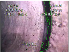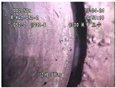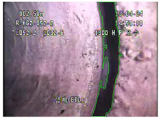
c6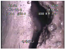
c7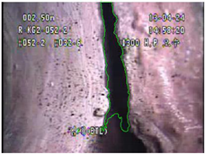
c10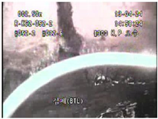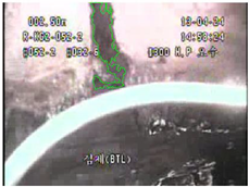
c15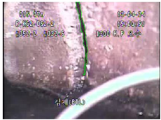
c22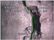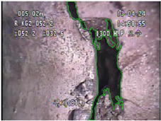

. Table 7 shows the comparison of the results by a statistical method, and the detected cracks are marked with a green outline on the original image. Gaussian statistic is analyzed to be superior in both quantitative and qualitative aspects. The reason for this is because the mean dilutes the edge. Thus, the neighboring Gaussian is analyzed to be effective.

3.2. User Algorithm

User algorithm is used to find cracks in Step 5 of Section 2, and it is a step to find only cracks in Step 4 of Table 2. As shown in

Table 8. Application of the user algorithm.

Original Image (c1)	Image at Step 4 (c1)
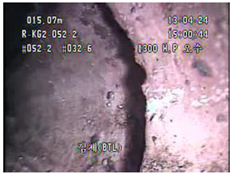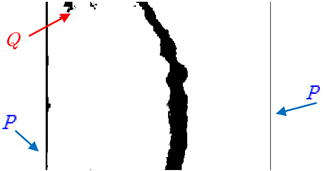Original Image (c16)	Image at Step 4 (c16)
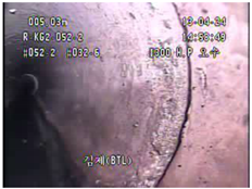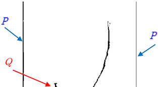Original Image (n15)	Image at Step 4 (n15)
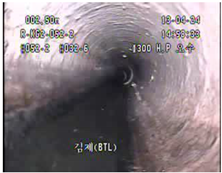Original Image (n23)	Image at Step 4 (n23)

, due to the low-resolution image characteristics of the sewer, it is detected like a crack in black on the left and right (the part marked with ‘P’). However, this is due to the idiosyncratic nature of the image, and in fact, it is not a crack. It should be removed.

The part marked with ‘Q’ in Table 8 is barely detected as a crack due to calculation error, but it is not a crack. To remove this error, the crack was detected by judging that the length and the width of the crack should be 9 mm (24 pixels) or more and 3 mm (eight pixels) or more, respectively. Additionally, if the width of the crack was more than half (160 pixels) of 320 pixels, which is the half of the width size of the image (240 × 320), it is determined that it is not a crack.

Table 9. User algorithm for crack detection.

Input: Image f(i, j) at Step 4 Output: Crack image g(i, j)       (1 ≤ i≤sz(1), 1 ≤ j ≤ sz(2))       (sz(1): Height of image, sz(2): width of image)
1	Using image f(j, i) in Step 4
2	for (k = 1 to No. of crack)
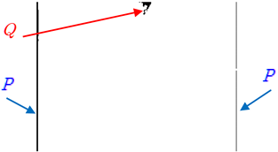
3	Truncate columns at left and right ends   (which are ‘P’ in Table 8)
4	for (i = 1 to sz(1))
5	Calculate length of cracks
6	end
7	for (j = 1 to sz(2))
8	Calculate width of cracks
9	end
10	Width of cracks     : longer than 3 mm (8 pixels) &, shorter than 160 pixels   Length of cracks     : More than 9 mm (24 pixel)
11	end

shows the algorithm for this step.

4. Results and Analysis

Through the crack detection procedure presented in Section 2 and the optimum parameters and user algorithm presented in Section 3, the crack detection results of the low-resolution sewer image were analyzed.

As a result of crack detection from the sewer images, 53 out of 55 (96.4%) were accurately detected as cracks, and 52 out of 55 (94.5%) were correctly detected as non-cracks.

Table 10. Summary of crack images.

	Images
Bad Results	c24, c52 (2 Images, 3.6%)
Good Results	c14, c16, c23, c25, c31, c32, c39, c40, c46, c51 (10 Images, 19.2%)
Excellent Results	Processed Image Count Excluding Upper Results (43 images, 78.2%)

and

Table 11. Summary of non-crack images.

	Images
Bad Results	n3, n5, n30 (3 Images, 5.4%)
Excellent Results	Processed Image Count Excluding Upper Results (52 images, 94.6%)

summarized the results of crack detection from crack and non-crack images, respectively. In Table 10, Bad results refer to detecting non-cracks as cracks, and Good results mean detecting only part of the crack. Excellent results refer to the case of perfect crack detection. Table 11 presents the results of crack detection from non-crack images only. If a crack is detected, when it is a non-crack image, it is considered a bad result. If it is correctly detected as not a crack, then it is an excellent result. Good results are meaningless in the case of non-crack images.

Table 12. Excellent results of crack images (only 12 results).

Original Image and Crack Image (c1)		Original Image and Crack Image (c3)
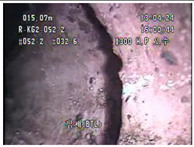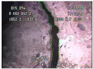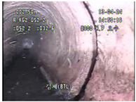Original Image and Crack Image (c4)		Original Image and Crack Image (c7)
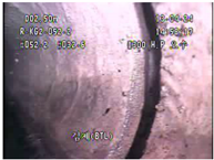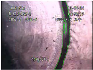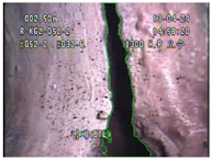Original Image and Crack Image (c8)		Original Image and Crack Image (c10)
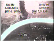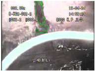Original Image and Crack Image (c15)		Original Image and Crack Image (c17)
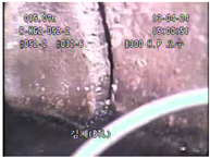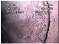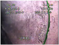Original Image and Crack Image (c20)		Original Image and Crack Image (c30)
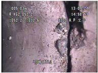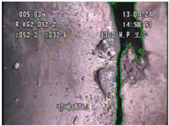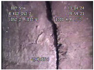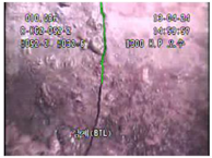Original Image and Crack Image (c47)		Original Image and Crack Image (c48)

shows the excellent results, and only 12 images are shown in consideration of the scope of paper size limit.

Table 13. Good results of crack images (all results).

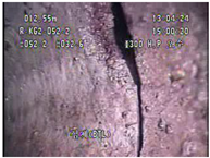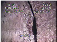Original Image and Crack Image (c14)		Original Image and Crack Image (c16)
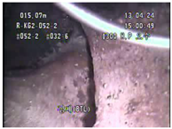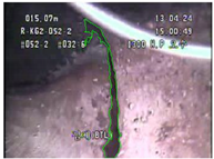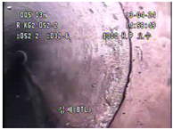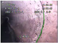Original Image and Crack Image (c23)		Original Image and Crack Image (c25)
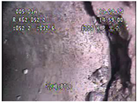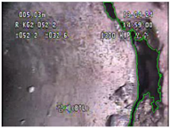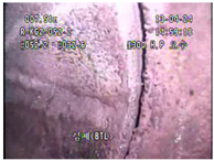Original Image and Crack Image (c31)		Original Image and Crack Image (c32)
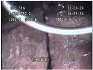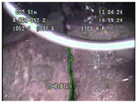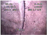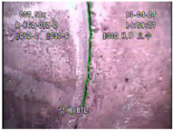Original Image and Crack Image (c39)		Original Image and Crack Image (c40)
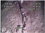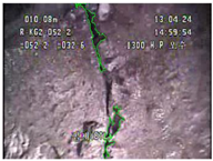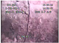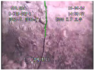Original Image and Crack Image (c46)		Original Image and Crack Image (c51)

shows the good results of detecting only a part of a crack.

Table 14. Bad results of crack and non-crack images (all results).

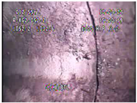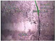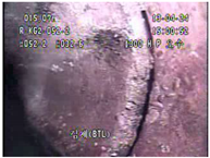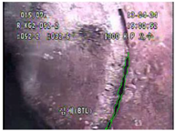Original Image and Crack Image (c24)		Original Image and Crack Image (c52)
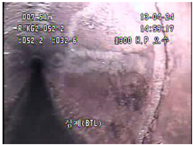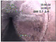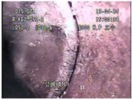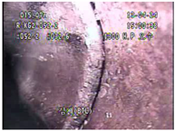Original Image and Non-Crack Image (n3)		Original Image and Non-Crack Image (n5)
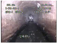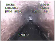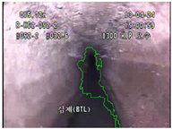
Original Image and Crack Image (n30)

shows the bad results of failing to detect cracks from crack images and the false detection of cracks from non-crack images.

5. Conclusions

This study improved the method of automatically detecting cracks from sewer images of very low resolution (240 × 320 = 76,800 pixels). Cracks were detected through a total of six steps such as enhancing the crack images in Step 2, finding the optimum threshold value in Step 3, and applying an algorithm to detect cracks in Step 5. Cracks were effectively detected by the optimum parameters obtained through Steps 2 and 3 and the user algorithm from Step 5.

Gaussian statistic is analyzed as superior in both quantitative and qualitative aspects. The reason for this is because the mean dilutes the edge. Thus, the neighboring Gaussian is analyzed to be effective. Despite the low resolution, the detection of crack images and non-crack images showed 96.4% accuracy and 94.5% accuracy with excellent quality, respectively. The accuracy is much higher than the results of the previous study by Son et al. [10], and the crack detection procedure is reduced from eight steps to six steps. In addition, the runtime taken to analyze one image was compared with the previous study [10]. This study took 0.103 s and the previous study [10] took 0.168 s. The runtime was reduced by 36.8%. Therefore, this study significantly advanced the previous study [10].

If the resolution of the image is increased (by at least 500,000 pixels) or an algorithm that effectively removes subtitles from the image is applied, cracks can be better detected. In conclusion, the findings of this study can be effectively used for the crack detection of low-resolution images.

References

- Xu, K.; Luxmoore, A.; Davies, T. Sewer pipe deformation assessment by image analysis of video surveys. Pattern Recognit. 1998, 31, 169–180. [Google Scholar] [CrossRef]
- McKim, R.A.; Sinha, S.K. Condition assessment of underground sewer pipes using a modified digital image processing paradigm. Tunn. Undergr. Space Technol. 1999, 14, 29–37. [Google Scholar] [CrossRef]
- Moselhi, O.; Shehab-Eldeen, T. Automated detection of surface defects in water and sewer pipes. Autom. Constr. 1999, 8, 581–588. [Google Scholar] [CrossRef]
- Yang, M.-D.; Su, T.-C. Automated diagnosis of sewer pipe defects based on machine learning approaches. Expert Syst. Appl. 2008, 35, 1327–1337. [Google Scholar] [CrossRef]
- Yang, M.-D.; Su, T.-C.; Pan, N.-F.; Yang, Y.-F. Systematic image quality assessment for sewer inspection. Expert Syst. Appl. 2011, 38, 1766–1776. [Google Scholar] [CrossRef]
- Sinha, S.K.; Fieguth, P.W. Automated detection of cracks in buried concrete pipe images. Autom. Constr. 2006, 15, 58–72. [Google Scholar] [CrossRef]
- Halfawy, M.R.; Hengmeechai, J. Efficient Algorithm for Crack Detection in Sewer Images from Closed-Circuit Television Inspections. J. Infrastruct. Syst. 2014, 20, 04013014. [Google Scholar] [CrossRef]
- Haurum, J.B.; Moeslund, T.B. A Survey on Image-Based Automation of CCTV and SSET Sewer Inspections. Autom. Constr. 2020, 111, 103061. [Google Scholar] [CrossRef]
- Son, B.J.; Jeon, J.R.; Heo, G.H. Image processing algorithm for crack detection of sewer with low resolution. J. Korea Acad. Ind. Coop. Soc. 2017, 18, 590–599. [Google Scholar]
- Heo, G.; Jeon, J.; Son, B. Crack Automatic Detection of CCTV Video of Sewer Inspection with Low Resolution. KSCE J. Civ. Eng. 2019, 23, 1219–1227. [Google Scholar] [CrossRef]
- Zuiderveld, K. Contrast Limited Adaptive Histograph Equalization, Graphic Gems IV; Academic Press Professional: San Diego, CA, USA, 1994; pp. 474–548. [Google Scholar]
- Bradley, D.; Roth, G. Adaptive Thresholding using the Integral Image. J. Graph. Tools 2007, 12, 13–21. [Google Scholar] [CrossRef]
- Soille, P. Morphological Image Analysis: Principles and Applications; Springer: Berlin/Heidelberg, Germany, 1999; pp. 173–174. [Google Scholar]
- Gonzalez, R.C.; Woods, R.E.; Eddins, S.L. Digital Image Processing Using MATLAB. Available online: http://www.gatesmark.com/ (accessed on 3 March 2021).