Abstract
Accurate measurement of honeybee (Apis mellifera) traffic in the vicinity of the hive is critical in systems that continuously monitor honeybee colonies to detect deviations from the norm. BeePIV, the algorithm we describe and evaluate in this article, is a new significant result in our longitudinal investigation of honeybee flight and traffic in electronic beehive monitoring. BeePIV converts frames from bee traffic videos to particle motion frames with uniform background, applies particle image velocimetry to these motion frames to compute particle displacement vector fields, classifies individual displacement vectors as incoming, outgoing, and lateral, and uses the respective vector counts to measure incoming, outgoing, and lateral bee traffic. We evaluate BeePIV on twelve 30-s color videos with a total frame count of 8928 frames for which we obtained the ground truth by manually counting every full bee motion in each frame. The bee motion counts obtained from these videos with BeePIV come closer to the human bee motion counts than the bee motion counts obtained with our previous video-based bee counting methods. We use BeePIV to compute incoming and outgoing bee traffic curves for two different hives over a period of seven months and observe that these curves closely follow each other. Our observations indicate that bee traffic curves obtained by BeePIV may be used to predict colony failures. Our experiments suggest that BeePIV can be used in situ on the raspberry pi platform to process bee traffic videos.
Dataset: The supplementary materials for our article include three video sets for the reader to appreciate how BeePIV processes bee traffic videos. Each set consists of three videos. The first video is an original raw video captured by our deployed BeePi electronic beehive monitoring system; the second video is the corresponding video that consists of the white background particle motion frames extracted from the first video; the third video is the video of displacement vectors extracted by PIV from each pair of consecutive white background frames from the second video. All computation is executed on a raspberry pi 3 model B v1.2 with four cores.
1. Introduction
Most of the work in a honeybee (Apis mellifera) colony is performed by the female worker bee whose average life span is approximately six weeks [1]. The worker becomes a forager in her third or fourth week after spending the first two to three weeks cleaning cells in the brood nest, feeding and nursing larvae, constructing new cells, receiving nectar, pollen, and water from foragers, and guarding the hive’s entrance. Foragers are worker bees mature enough to leave the hive for pollen, nectar, and water [2] and, when necessary, as scouts in search of new homesteads when their colonies prepare to split through swarming [3].
Since robust forager traffic is an important indicator of the well-being of a honeybee colony, accurate continuous measurement of honeybee traffic in the vicinity of the hive is critical in electronic beehive monitoring (EBM) systems that monitor honeybee colonies to detect and report deviations from the norm [4]. In a previous article [5], we presented our first algorithm based on particle image velocimetry (PIV) to measure directional honeybee traffic in the vicinity of a Langstroth hive [6]. We proposed to classify bee traffic in the vicinity of the hive as incoming, outgoing, and lateral. Incoming traffic consists of bees entering the hive through the landing pad or round holes in hive boxes (also known as supers). Outgoing traffic consists of bees leaving the hive either from the landing pad or from box holes. Lateral traffic consists of bees flying, more or less, in parallel to the front side of the hive (i.e., the side with the landing pad). We proposed to refer to these three types of traffic as directional traffic and defined omnidirectional traffic as the sum of the measurements of incoming, outgoing, and lateral traffic [7].
In this article, we present BeePIV, a video-based algorithm to measure omnidirectional and directional honeybee traffic. The algorithm is a new significant result in our ongoing longitudinal investigation of honeybee flight and traffic in images and videos acquired with our deployed BeePi EBM systems [5,7,8,9]). BeePIV is a significant improvement of our previous algorithm [5]. Our previous algorithm applied PIV directly to raw video frames without converting them to frames with uniform background or clustering multiple motion points generated by a single bee into a single particle, which had a negative effect on its accuracy. In BeePIV, frames from bee traffic videos are converted to particle motion frames with uniform white background and multiple motion points generated by a single bee are clustered into a single particle. PIV is applied to these particle motion frames to compute particle displacement vector fields. Individual displacement vectors are classified as incoming, outgoing, and lateral, and the respective vector counts are used to measure incoming, outgoing, and lateral bee traffic.
BeePIV is guided by our conjecture that there exist functions that map color variation in videos to video-specific threshold and distance values that can be used to reduce smoothed difference frames to uniform background frames with motion points. Another conjecture that we have implemented and partially verified in BeePIV is that color variation can be used to estimate optimal interrogation window sizes and overlaps for PIV.
We evaluate BeePIV on twelve 30-s color videos with various levels of bee traffic for which we obtained the ground truth by manually counting every full bee motion in each frame, which also constitutes a significant improvement on the evaluation of the previous algorithm whose performance was evaluated only on four 30-s videos. Another critical difference is that our previous algorithm when tested on the raspberry pi 3 model B v1.2 platform on 30-s videos, had an unacceptably slow performance of ≈2.5 h per video. BeePIV, by contrast, has a mean processing time of 2.15 min with a standard deviation of 1.03 min per video when tested on the same raspberry pi 3 model B v1.2 platform.
The remainder of our article is organized as follows. In Section 2, we present related work. In Section 3, we describe the hardware of the BeePi monitors we built and deployed on Langstroth hives to acquire bee traffic videos for this investigation and give a detailed description of BeePIV. In Section 4, we present the experiments we designed to evaluate the proposed algorithm. In Section 5, we summarize our observations and findings.
2. Related Work
While PIV is one of the most important measurement methods in fluid dynamics [10,11], it has also been used to measure and characterize insect flight patterns and topologies, because flying insects leave behind air motions that can be captured in regular or digital photos. PIV analysis of flight patterns improves our understanding of the insects’ behavior and ecology.
Several research groups have used PIV to investigate insect flight. Dickinson et al. [12] applied PIV to measure fluid velocities of a fruit fly and to determine the contribution of the leading-edge vortex to overall force production. Bomphrey et al. [13] performed a detailed PIV analysis of the flow field around the wings of the tobacco hawkmoth (Manduca sexta) in a wind tunnel. Flow separation was associated with a saddle between the wing bases on the surface of the hawkmoth’s thorax. Michelsen [14] used PIV to examine and analyze sound and air flows generated by dancing honeybees. PIV was used to map the air flows around wagging bees. It was discovered that the movement of the bee’s body is followed by a thin (1–2 mm) boundary layer and other air flows lag behind the body motion and are insufficient to fill the volume left by the body or remove the air from the space occupied by the bee body. The PIV analysis showed that flows collide and lead to the formation of short-lived eddies.
Several video-based electronic beehive monitoring (EBM) projects are related to our research. Rodriguez et al. [15] proposed a system that uses trajectory tracking to distinguish entering and leaving bees, which works reliably under smaller bee traffic levels. The dataset used by the researchers to evaluate their system consists of 100 fully annotated frames, where each frame contains 6–14 honeybees. Babic et al. [16] proposed a system for pollen bearing honeybee detection in videos obtained at the entrance of a hive. The system’s hardware includes a specially designed wooden box with a raspberry pi camera module inside. The box is mounted on the front side of a standard hive above the hive entrance. A glass plate is placed on the bottom side of the box, 2 cm above the flight board, which forces the bees entering or leaving the hive to crawl a distance of ≈11 cm. Consequently, the bees in the field of view of the camera cannot fly. The training dataset contained 50 images of pollen bearing honeybees and 50 images of honeybees without pollen. The test dataset consisted of 354 honeybee images.
The research reported in this article has been influenced and inspired by our ongoing research and development work on the mobile instructional particle image velocimetry (mI-PIV) system [17,18]. The system uses a smartphone’s internal camera for image acquisition and performs PIV analysis either on a web server or directly on the smartphone running Android using both open-source and our own PIV algorithms. We have been investigating the effects of different PIV parameters on the accuracy of the mI-PIV system. This system is an innovative stepping stone in making PIV less expensive and more widely available, particularly for application within educational settings. Our main design objective is to achieve convenience and safety without sacrificing too much accuracy so that the system is available not only to physics, engineering, and computer science university majors and professionals but also to high school students who have never had any exposure to PIV due to the expensive nature of commercial PIV systems.
We have designed and completed various experiments to benchmark the mI-PIV system as part of our iterative design-based research process. Our main findings are: (1) average flow velocity appears to be positively correlated with error due to higher in-plane gradients, particle streaking, greater in-plane motion of particles, and greater out-of-plane motion of particles associated with higher flow velocities; (2) while the mean bias error of different open-source PIV algorithms (e.g., OpenPIV [19], JPIV [20], and PIVLab [21]) varies, the variations are not significant to have appreciable effects on the overall accuracy on synthetic images; (3) the overall physical image processing times of the web server-based (images from fluid low videos are taken on a smartphone and processed on a web server) and smartphone-based (image capture and processing is done on a smartphone running Android) implementations of the mI-PIV system are similar with the smartphone-based implementation’s mean processing time being slightly smaller.
3. Materials and Methods
3.1. Hardware and Data Acquisition
The video data for this investigation were captured by BeePi monitors, multi-sensor EBM systems we designed and built in 2014 [8], and have been iteratively modifying since then [7,22]. Each BeePi monitor (see Figure 1) consists of a raspberry pi 3 model B v1.2 computer, a pi T-Cobbler, a breadboard, a waterproof DS18B20 temperature sensor, a pi v2 8-megapixel camera board, a v2.1 ChronoDot clock, and a Neewer 3.5 mm mini lapel microphone placed above the landing pad. All hardware components fit in a single Langstroth super. BeePi units are powered either from the grid or rechargeable batteries.
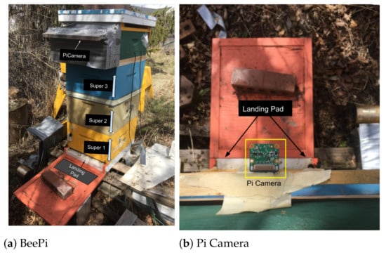
Figure 1.
BeePi monitor (a) on top of Langstroth beehive of 3 supers; BeePi’s hardware components are in top green super; pi camera (b) is looking down on landing pad and is protected against elements by wooden box; hardware details and assembly videos are available at [23,24].
BeePi monitors thus far have had six field deployments. The first deployment was in Logan, UT (September 2014) when a single BeePi monitor was placed into an empty hive and ran on solar power for two weeks. The second deployment was in Garland, UT (December 2014–January 2015), when a BeePi monitor was placed in a hive with overwintering honeybees and successfully operated for nine out of the fourteen days of deployment on solar power to capture ≈200 MB of data. The third deployment was in North Logan, UT (April–November 2016) where four BeePi monitors were placed into four beehives at two small apiaries and captured ≈20 GB of data. The fourth deployment was in Logan and North Logan, UT (April–September 2017), when four BeePi units were placed into four beehives at two small apiaries to collect ≈220 GB of audio, video, and temperature data. The fifth deployment started in April 2018, when four BeePi monitors were placed into four beehives at an apiary in Logan, UT. In September 2018, we decided to keep the monitors deployed through the winter to stress test the equipment in the harsh weather conditions of northern Utah. By May 2019, we had collected over 400 GB of video, audio, and temperature data. The sixth field deployment started in May 2019 with four freshly installed bee packages and is still ongoing as of January 2021 with ≈250 GB of data collected so far. In early June 2020, we deployed a BeePi monitor on a swarm that made home in one of our empty hives and have been collecting data on it since then.
We should note that, unlike many apiarists, we do not intervene in the life cycle of the monitored hives in order to preserve the objectivity of our data and observations. For example, we do not apply any chemical treatments to or re-queen failing or struggling colonies.
3.2. Terminology, Notation, and Definitions
We use the terms frame and image interchangeably to refer to two-dimensional (2D) pixel matrices where pixels can be either real non-negative numbers or, as is the case with multi-channel images (e.g., PNG or BMP), tuples of real non-negative numbers.
We use pairs of matching left and right parentheses to denote sequences of symbols. We use the set-theoretic membership symbol ∈ to denote when a symbol is either in a sequence or in a set of symbols. We use the universal quantifier ∀ to denote the fact that some mathematical statement holds for all mathematical objects in a specific set or sequence and use the existential quantifier ∃ to denote the fact that some mathematical statement holds for at least one object in a specific set or sequence.
We use the symbols ∧ and ∨ to refer to the logical and and the logical or, respectively. Thus, states a common truism that for every natural number i there is another natural number j greater than i.
Let and be sequences of symbols, where are positive integers. We define the intersection of two symbolic sequences in Equation (1), where are positive integers, whenever , for and . If two sequences have no symbols in common, then .
We define a video to be a sequence of consecutive equi-dimensional 2D frames , where t, j, and k are positive integers such that . Thus, if a video V contains 745 frames, then = , . By definition, videos consist of unique frames so that if and , then . It should be noted that and may be the same pixelwise. Any smaller sequence of consecutive frames of a larger video is also a video. For example, if is a video, then so are and .
When we discuss multiple videos that contain the same frame symbol or when we want to emphasize specific videos under discussion, we use superscripts in frame symbols to reference respective videos. Thus, if videos and include , then designates in and designates in .
Let be a video, , and be a positive integer. A frame’s context in V, denoted as , is defined in Equation (2).
where
In other words, the context of is a video that consists of a sequence of consecutive or fewer frames (possibly empty) that precede and a sequence of or fewer frames (possibly empty) that follow it. We refer to as a context size and to as the -context or, simply, context of and refer to as the contextualized frame of . If there is no need to reference V, we omit the superscript and refer to as the contextualized frame of .
For example, let , then the 3-context of is
Analogously, the 2-context of is
If , then is the pixel value at row r and column c in . If is a frame whose pixel values at each position are real numbers, we use the notation to refer to the maximum such value in the frame. If , then the mean frame of V, denoted as or when V can be omitted, is the frame where the pixel value at is the mean of the pixel values at of all frames , as defined in Equation (3).
If pixels are n-dimensional tuples (e.g., each is an RGB or PNG image), then each pixel in is an n-dimenstional tuple of the means of the corresponding tuple values in all frames .
Let be a video, and let be a context size and be the context of . The l-th dynamic background frame of V, denoted as , , is defined in Equation (4) as the mean frame of (i.e., the mean frame of the -context of ).
In general, the dynamic background operation specified in Equation (4) is designed to filter out noise, blurriness, and static portions of the images in a given video. As the third video set in the supplementary material shows, BeePIV can process videos taken against the background of grass, trees, and bushes. For an example, consider a 12-frame video V in Figure 2, and let . Figure 3 shows 12 dynamic background frames for the video in Figure 2. In particular, is the mean frame of of ; is the mean frame of of ; is the mean frame of of ; and is the mean frame of of . Proceeding to the right in this manner, we reach , the last contextualized frame of V, which is the mean frame of of .
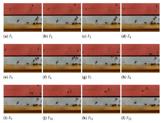
Figure 2.
Twelve frames of a video .
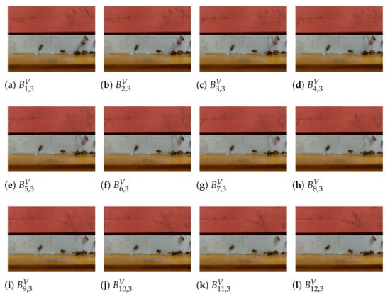
Figure 3.
Twelve dynamic background frames of video V in Figure 2 with .
A neighborhood function maps a pixel position in to a set of positions around it. In particular, we define two neighborhood functions (see Equation (5)) and (see Equation (6)) for the standard 4- and 8-neighborhoods, respectively, used in many image processing operations. Given a position in , the statement states that the 8-neighborhood of includes a position such that and .
We use the terms PIV and digital PIV (DPIV) interchangeably as we do the terms bee and honeybee. Every occurrence of the term bee in the text of the article refers to the Apis Mellifera honeybee and to no other bee species. We also interchange the terms hive and beehive to refer to a Langstroth beehive hosting an Apis Mellifera colony.
3.3. BeePIV
3.3.1. Dynamic Background Subtraction
Let be a video. In BeePIV, the background frames are subtracted pixelwise from the corresponding contextualized frames to obtain difference frames. The l-th difference frame of V, denoted as , is defined in Equation (7).
The pixels in that are closest to the corresponding pixels in represent positions that have remained unchanged over a specific period of physical time over which the frames in were captured by the camera. Consequently, the positions of the pixels in where the difference is relatively high, signal potential bee motions. Figure 4 shows several difference frames computed from the corresponding contextualized and background frames of the 12-frame video in Figure 2.
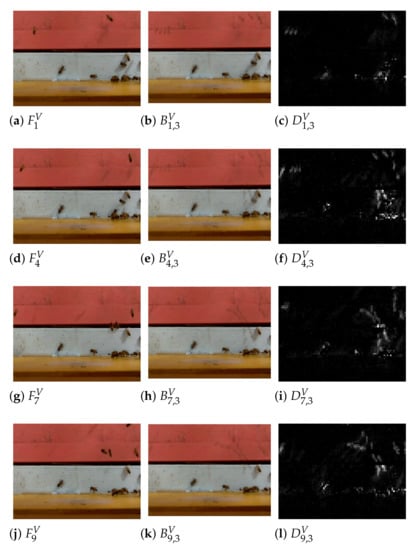
Figure 4.
Difference frames , for , computed from contextualized frames , , , and corresponding background frames , , , of 12-frame video V in Figure 2.
3.3.2. Difference Smoothing
A difference frame may contain not only bee motions detected in the corresponding contextualized frame but also bee motions from the other frames in the context or motions caused by flying bees’ shadows or occasional blurriness. In BeePIV, smoothing is applied to to replace each pixel with a local average of the neighboring pixels. Insomuch as the neighboring pixels measure the same hidden variable, averaging reduces the impact of bee shadows and blurriness without necessarily biasing the measurement, which results in more accurate frame intensity values. An important objective of difference smoothing is to concentrate intensity energy in those areas of that represent actual bee motions in .
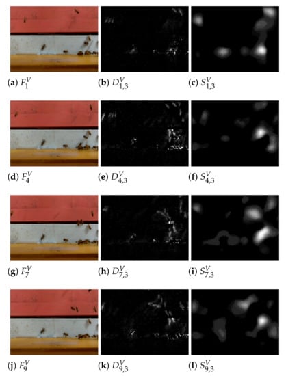
The smoothing operator, , is defined in Equation (9), where is a real positive number and is a weighting function assigning relative importance to each neighborhood position. In the current implementation of BeePIV, . We will use the notation to denote the smoothed difference frame obtained from so that . We will use the notation as a shorthand for the application of to every position in to obtain . Figure 5 shows several smoothed difference frames obtained from the corresponding difference frames where the weights are assigned using the weight function in Equation (10).
Let and let . The video smoothing operator applies the smoothing operator H to every frame in and returns a sequence of smoothed difference frames , as defined in Equation (11), where is a sequence of difference frames.
3.3.3. Color Variation
Since a single flying bee may generate multiple motion points in close proximity as its body parts (e.g., head, thorax, and wings) move through the air, pixels in close proximity (i.e., within a certain distance) whose values are above a certain threshold in smoothed difference frames can be combined into clusters. Such clusters can be reduced to single motion points on a uniform (white or black) background to improve the accuracy of PIV. Our conjecture, based on empirical observations, is that a video’s color variation levels and its bee traffic levels are related and that video-specific thresholds and distances for reducing smoothed difference frames to motion points can be obtained from video color variation.
Let be a video and let (see Equation (4)) be the background frame of with (i.e., the number of frames in V). To put it differently, as Equation (4) implies, is the mean frame of the entire video and contains information about regions with little or no variation across all frames in V.
A color variation frame, denoted as (see Equation (12)), is computed for each as the squared smoothed pixelwise difference between and across all image channels.
The color variation values from all individual color variation frames are combined into one maximum color variation frame, denoted as (see Equation (13)), for the entire video V. Each position in holds the maximum value for across all color variation frames , where . In other words, contains quantized information for each pixel position on whether there has been any change in that position across all frames in the video.
Figure 6 gives the background and maximum color variation frames for a low bee traffic video and a high bee traffic video . The maximum color variation frames are grayscale images whose pixel values range from 0 (black) to 255 (white). Thus, the whiter the value of a pixel in a is, the greater the color variation at the pixel’s position. As can be seen in Figure 6, has fewer whiter pixels compared to and the higher color variation clusters in tend to be larger and more evenly distributed across the frame than the higher color variation clusters in .
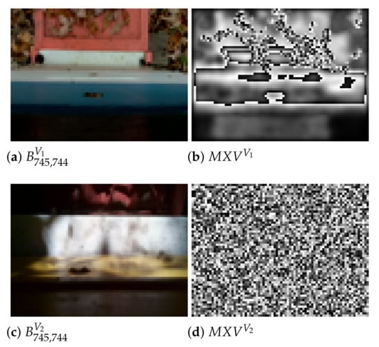
Figure 6.
is a low bee traffic video with 745 frames; is the background frame of ; is the maximum color variation frame for ; is a high bee traffic video with 745 frames; is the background frame of ; is maximum color variation frame for .
The color variation of a video V, denoted as , is defined in Equation (14) as the standard deviation of the mean of . Higher values of indicate multiple motions; lower values indicate either relatively few motions or complete lack thereof. We intend to investigate this implication in our future work.
We postulate in Equation (15) the existence of a function from reals to 2-tuples of reals that maps color variation values for videos (i.e., ) to video-specific threshold and distance values that can be used to reduce smoothed difference frames to uniform background frames with motion points. In Section 4.2, we define one such function in Equation (33) and evaluate it in Section 4.3, where we present our experiments on computing the PIV interrogation window size and overlap from color variation.
Suppose there is a representative sample of bee traffic videos obtained from a deployed BeePi monitor. Let and be experimentally observed lower and upper bounds, respectively, for the values of . In other words, for any , . Let and be the experimentally selected lower and upper bounds, respectively, for , that hold for all videos in the sample. Then in Equation (15) can be constrained to lie between and , as shown in Equation (16).
The frame thresholding operator, , is defined in Equation (17), where, for any position in , if and , otherwise. The video thresholding operator, , applies to every frame in and returns a sequence of smoothed tresholded difference frames , as defined in Equation (18), where .
In Section 4.2, we give the actual values of and we found by experimenting with the videos on our testbed dataset. Figure 7 shows the background frame of the video in Figure 2 and the value of computed from for the video. Figure 8 shows the impact of smoothing difference frames with the smoothing operation H (see Equation (9)) and then thresholding them with computed from .
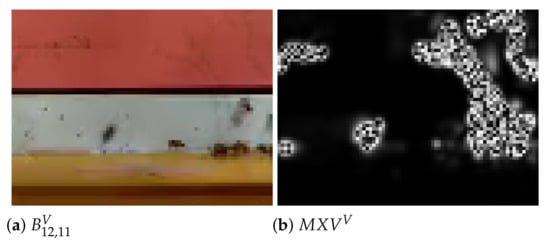
Figure 7.
Background frame (a) for 12 frames of video V in Figure 2 and (b) corresponding for V that holds values and positions of highest color variations across all 12 frames in V; value of computed from is 13.59; value of is 11.35; is computed by function in Equation (33) in Section 4.2.
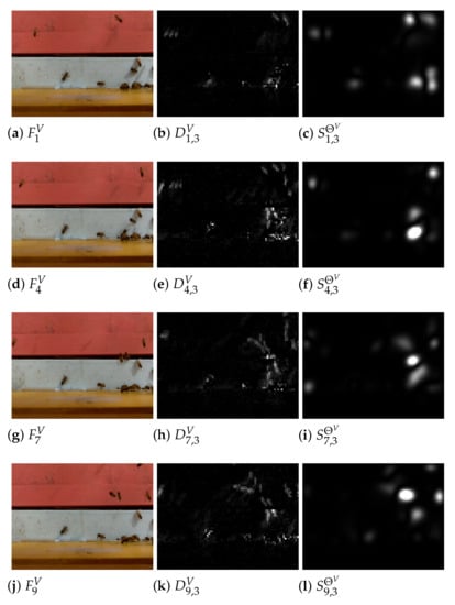
Figure 8.
Frames in left column are from video V in Figure 2; frames in middle column are corresponding difference frames computed from frames in left column; frames are computed from corresponding frames in middle column by smoothing them and thresholding their pixel values at .
The values of are used to threshold smoothed difference frames from a video V and the values of , as we explain below, are used to determine which pixels are in close proximity to local maxima and should be eroded. Higher values of indicate the presence of higher bee traffic and, consequently, must be accompanied by smaller values between maxima points, because in higher traffic videos, multiple bees fly in close proximity to each other. On the other hand, lower values of indicate lower traffic and must be accompanied by higher values of , because in lower traffic videos bees typically fly farther apart.
3.3.4. Difference Maxima
Equation (19) defines a maxima operator that returns 1 if a given position in a smooth thresholded difference frame is a local maxima by using the neighborhood function in Equation (5). By analogy, we can define , another maxima operator to do the same operation by using the neighborhood function in Equation (6).
We will use the notation , where n is a positive integer (e.g., or ), as a shorthand for the application of to every position of in to obtain the frame . The symbol b in the subscript of indicates that this frame is binary, where, per Equation (19), 1’s indicate positions of local maxima. Figure 9 shows that application of to a smoothed difference frame to obtain the corresponding .
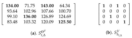
Figure 9.
(a) Smoothed thresholded difference frame ; (b) ; positions of local maxima in are (1,1), (1,3), (3,2), and (4,4); the values at these positions in are bolded.
The video maxima operator applies the maxima operator to every frame in a sequence of smoothed thresholded difference frames , and returns a sequence of binary difference frames, as defined in Equation (20), where is a sequence of smoothed thresholded difference frames.
3.3.5. Difference Maxima Erosion
Let P be the sequence of positions of all maxima points in the frame . For example, in Figure 9, . We define an erosion operator that, given a distance , constructs the set P, sorts the positions in P by their i coordinates, and, for every position such that , sets the pixel values of all the positions that are within pixels of in to 0 (i.e., erodes them). We let refer to the smoothed and eroded binary difference frame obtained from after erosion and define the erosion operator E in Equation (21).
The application of the erosion operator is best described algorithmically. Consider the binary difference frame in Figure 10a. Recall that this frame is the frame in Figure 9b obtained by applying the maxima operator to the frame in Figure 9a. After is applied, the sequence of the local maxima positions is .
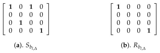
Figure 10.
(a) Binary difference frame ; (b) eroded frame , where and .
Let us set the distance parameter of the erosion operator to 4 and compute . As the erosion operator scans left to right, the positions of the eroded maxima are saved in a dynamic lookup array (let us call it I) so that the previously eroded positions are never processed more than once. The array I holds the index positions of the sorted pixel values at the positions in P. Initially, in our example, , because the pixel values at the positions in P, sorted from lowest to highest, are so that the value 125.50 is at position 4 in P, the value 134.00 at position 1, the value 136.00 at position 3, and the value 143 at position 2. In other words, the pixel value at is the lowest and the pixel value at the highest. For each value in I which has not yet been processed, the erosion operator computes the euclidean distance between its coordinates and the coordinates of each point to the right of it in I that has not yet been processed. For example, in the beginning, when the index position is at 1, the operator computes the distances between the coordinates of position 1 and the coordinates of positions 2, 3, and 4.
If the current point in I is at , a point to the left of it in I is at , then is the distance between them. If , the point at is eroded and is marked as such. The erosion operator continues to loop through I, skipping the indices of the points that have been eroded. In this example, the positions 2 and 3 in P are eroded. Thus, the frame shown in Figure 10b, has 1’s at positions and and 0’s everywhere else.
Since the erosion operator is greedy, it does not necessarily ensure the largest pixel values are always selected, because their corresponding positions may be within the distance of a given point whose value may be lower. In our example, the largest pixel value 143 at position is is eroded, because it is within the distance threshold from , which is considered first.
A more computationally involved approach to guarantee the preservation of relative local maxima is to sort the values in in descending order and continue to erode the positions within pixels of the position of each sorted maxima until there is nothing else to erode. In practice, we found that this method does not contribute to the accuracy of the algorithm due to the proximity of local maxima to each other. To put it differently, it is the positions of the local maxima that matter, not their actual pixel values in smoothed difference frames in that the motion points generated by the multiple body parts of a flying bee have a strong tendency to cluster in close proximity.
The video erosion operator applies the erosion operator to every frame in a sequence of binary difference frames and returns a sequence of corresponding eroded frames , as defined in Equation (22), where is a sequence of difference frames.
The positions of 1’s in each are treated as centers of small circles whose radius is of the width of , where in our current implementation. The parameter, in effect, controls the size of the motion points for PIV. After the black circles are drawn on a white background the frame becomes the frame . We refer to frames as motion frames and define the drawing operator in Equation (23), where is obtained by drawing at each position with 1 in a black circle with a radius of of the width of .
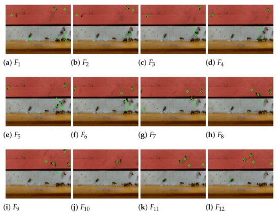
Figure 11 shows twelve motion frames obtained from the twelve frames in Figure 2. Figure 12 shows the detected motion points in each motion frame plotted on the corresponding original frame from which was obtained. The motion frames record bee motions reduced to single points and constitute the input to the PIV algorithm described in the next section.
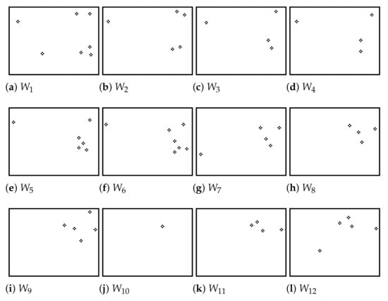
Figure 11.
Motion frames to obtained from original frames to in Figure 2.
The video drawing operator applies the drawing operator to every frame in a sequence of eroded frames and returns a sequence of the corresponding white background frames with black circles , as defined in Equation (24), where is a sequence of eroded frames. The sequence of motion frames is given to the PIV algorithm described in the next section.
3.3.6. PIV and Directional Bee Traffic
Let be a sequence of motion frames and let and be two consecutive motion frames in this sequence that correspond to original video frames and . Let be a window, referred to as interrogation area or interrogation window in the PIV literature, selected from and centered at position . Another window, , is selected in so that . The position of in is the function of the position of in in that it changes relative to to find the maximum correlation peak. For each possible position of in , a corresponding position is computed in .
The 2D matrix correlation is computed between and with the formula in Equation (25), where are integers in the interval . In Equation (25), and are the pixel intensities at locations in and in . For each possible position of inside , the correlation value is computed. If the size of is and the size of is , then the size of the matrix C is .
The matrix C records the correlation coefficient for each possible alignment of with . A faster way to calculate correlation coefficients between two image frames is to use the Fast Fourier Transform (FFT) and its inverse, as shown in Equation (26). The reason why the computation of Equation (26) is faster than the computation of Equation (25) is that and must be of the same size.
If is the maximum value in C and is the center of , the pair of and defines a displacement vector from in to in . This vector represents how particles may have moved from to . The displacement vectors form a vector field used to estimate possible flow patterns.
Figure 13 shows two frames and , two corresponding motion frames and obtained from them by the application of the operator in Equation (24), and the vector field computed from and by Equation (26). The two displacement vectors correspond to the motions of two bees with the left bee moving slightly left and the right bee moving down and right.
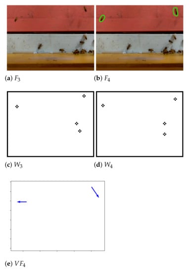
In Equation (27), we define the PIV operator that applies to two consecutive motion frames and to generate a field of displacement vectors . The video PIV operator applies the PIV operator G to every pair of consecutive motion frames and in a sequence of motion frames and returns a sequence of vector fields , as defined in Equation (28), where is a sequence of eroded frames. It should be noted that the number of motion frames in Z exceeds the number of the vector fields returned by the video PIV operator by exactly 1.
After the vector fields are computed by the G operator for each pair of consecutive motion frames and , the directions of the displacement vectors are used to estimate directional bee traffic. Each vector is classified as lateral, incoming, or outgoing according to the value ranges in Figure 14. A vector is classified as outgoing if its direction is in the range , as incoming if its direction is in the range , and as lateral otherwise.
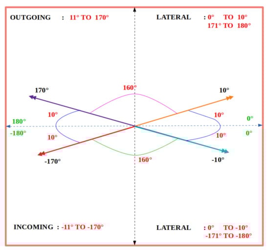
Figure 14.
Degree ranges used to classify PIV vectors as lateral, incoming, and outgoing.
Let and be two consecutive motion frames from a video V. Let , , and be the counts of incoming, outgoing, and lateral vectors. If is a sequence of k motion frames obtained from V, then , , and can be used to define three video-based functions , , and that return the counts of incoming, outgoing, and lateral displacement vectors for Z, as shown in Equation (29).
For example, let such that , , and , , . Then, , , and .
We define the video motion count operator in Equation (30) as the operator that returns a 3-tuple of directional motion counts obtained from a sequence of motion frames Z with , , and .
3.3.7. Putting It All Together
We can now define the BeePIV algorithm in a single equation. Let be a video. Let the video’s color variation (i.e., ) be computed with Equation (14) and let the values of , and be computed from with Equation (15). We also need to select a context size and the parameter for the circle drawing operator in Equation (24) to generate motion frames .
The BeePIV algorithm is defined in Equation (31) as the operator that applies to a video V. The operator is a composition of operators where each subsequent operator is applied to the output of the previous one. The operator starts by applying the video difference operator in Equation (8) to subtract from each contextualized frame its background frame . The output of is given to the video smoothing operator in Equation (11). The smoothed frames produced by are given to the video maxima operator in Equation (20) to detect positions of local maxima. The frames produced by are given to the video erosion operator in Equation (22). The eroded frames produced by are processed by the video drawing operator in Equation (24) that turns these frames into white background motion frames and gives them to the video motion count operator in Equation (30) to return the counts of incoming, outgoing, and lateral displacement vectors. We refer to Equation (31) as the BeePIV equation. Figure 15 gives a flowchart of the BeePIV algorithm.
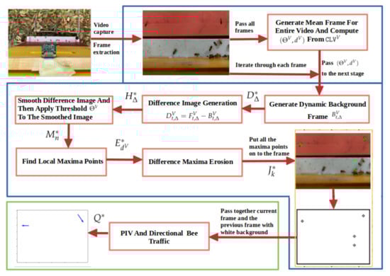
Figure 15.
Flowchart of BeePIV.
4. Experiments
4.1. Curated Video Data
We used thirty-two 30-s videos for our experiments from two BeePi monitors. Both monitors were deployed in an apiary in Logan, Utah, USA from May to November 2018. The raw videos captured by BeePi monitors have a resolution of 1920 × 1080 pixels, H.264 Codec, and a frame rate of 25 frames per second. In our current implemented version of BeePIV with which we performed the experiments described in this section, each video frame is resized to a resolution of 60 × 80 for faster processing on the raspberry pi platform.
We selected the videos to reflect varying levels of bee traffic across different backgrounds and under different weather conditions. Of these videos, we randomly selected 20 videos for our experiments to obtain plausible, data-driven parameters for the function in Equation (15) and in Equation (16) and evaluate the experimental findings on the remaining 12 videos. We refer to the set of 20 videos as the testbed set and to the set of 12 videos as the evaluation set. By using these terms we seek to avoid confusion with the terms training set and testing set prevalent in the machine learning literature, because BeePIV does not use machine learning techniques.
For ease of reference and interpretation of the plots in this section, we explicitly state that our testbed consisted of videos 5–8 and videos 10–25 and our evaluation set consisted of videos 1–4, 9, and 26–32. Since our testbed set contained 20 videos, each of which had 744 frames with the raspberry pi camera’s frame capture rate of ≈25 frames per second, the total frame count for this set was 14,880 (i.e., ). Since our evaluation set included 12 color videos, each of which had 744 frames, the total frame count for this set was 8928 (i.e., ).
For each video in both sets, we manually counted full bee motions in each frame and took the number of bee motions in the first frame of each video (Frame 1) to be 0. A full bee motion occurs when the entire body of a bee (tail, thorax, wings, head) moves from frame to frame. If a bee’s head or tail appears in a frame, it is not considered a full bee motion. In each subsequent frame, we counted the number of full bees that moved when compared to their positions in the previous frame. We also counted as full bee motions in a given frame (except in Frame 1) bees flying into the camera’s field of view that were abscent in the previous frame.
For 27 out of the 32 videos we also marked each moving bee with polygons of different colors easily distinguishable from the background, as shown in Figure 16, for faster verification of each other’s counts. We compiled a CSV file for each curated video with a count of bee motions in each frame. For example, the CSV file for the video out of which the two frames in Figure 16 were taken, has entries 2 for and 3 for , because has 2 marked bee motions and has 3 marked bee motions. It took us ≈10 h to curate each video for a total of ≈320 h of manual video curation. Higher traffic videos took, on average, 2–3 h longer to curate than lower traffic videos. We used the 32 CSV files with manual bee motion counts as the ground truth for our experiments. In all 32 videos, we identified 25,090 full bee motions: 20,590 motions in the testbed dataset and 4500 in the evaluation dataset.
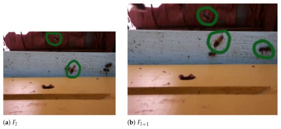
Figure 16.
Two consecutive curated frames from a BeePi video; in both frames each full bee motion was marked by a human curator with a green polygon.
4.2. Color Variation Threshold and Erosion Distance
We re-state, for ease of reference, Equation (14) for the color variation of a video V and Equation (16) for the color variation’s scaled threshold .
When we computed for each video in the testbed set, we observed that the rounded values of ranged from 5 to 210 and set to 5 and to 210. We also observed that for all of the videos the rounded values of ranged from 9 to 65. In particular, for the videos with lower bee traffic, tended toward 9 and for the videos with higher bee traffic–toward 65. Thus, we set the values of and to 9 and 65, respectively. Consequently, in the current implementation of BeePIV, the value of is computed according to Equation (32).
Recall that in Equation (15) we postulated the existence of functions from reals to 2-tuples of reals that maps video-specific color variation values to video-specific color variation threshold and erosion distance values that are used to convert smoothed difference frames to motion frames with uniform background. In the current implementation of BeePIV, the function is computed in accordance with Equation (33).
where
In Equation (33), we chose the specific ranges for in on the basis of our experiments with the 20 videos in the testbed set. We observed that the values computed from the videos with lower to medium bee traffic ranged from 9 to ≈21.5 and for the videos with medium to higher traffic ranged from 22 to 65. The average size of an individual honey bee in 60 × 80 video frames that BeePIV processes is ≈10 pixels. In lower traffic videos, where bees do not tend to fly in close proximity, we chose to set the value of to approximately 1/2 the size of the bee so that local maxima positions that farther apart than half the bee are not eroded. In higher traffic videos, where bees tend to fly in closer proximity, we set the value of to approximately 1/3 the size of the bee so that local maxima positions that are farther apart than a third of the bee are not eroded.
4.3. Interrogation Window Size and Overlap in PIV
To estimate the optimal values for the interrogation window size (i.e., the size of and ) and window overlap (see Equation (26)), we ran a grid search on the videos in the testbed set. Since we use the FFT version of the correlation equation, and are of the same size in BeePIV.
For the grid search, we tested all interrogation windows, where , in increments of 1. We chose values for the grid search, because the mean size of an individual honey bee is ≈10 pixels. Thus, the dimension of the smallest interrogation window is two pixels below the mean bee’s size and the dimension of the largest interrogation window is almost twice the mean bee’s size.
The control flow of the grid search was as follows. For each video V in the testbed set, for each window size in the interval , for each overlap from 1% to 70%, we used the BeePIV Equation (see Equation (31)) to compute the counts of incoming, outgoing, and lateral displacement vectors (i.e., , respectively). For each video, the overall omnidirectional count was computed as and was compared with the human ground truth count for the video in the corresponding CSV file. The absolute difference between the BeePIV count and human count (i.e., the absolute error) was recorded. Table 1 gives the interrogation window size and overlap for each video that resulted in the smallest absolute error for that video.

Table 1.
Interrogation window size and overlap for each video in testbed that resulted in smallest absolute error between BeePIV and human counts for that video; values in BeePIV column are , where Z is motion frame sequence of corresponding video V; values in Err column are absolute differences between corresponding values in Human Count and BeePIV columns.
On the basis of the grid search, we designed two functions , defined in Equation (34), and , defined in Equation (35), to map color variation (i.e., ) to 2-tuples of interrogation window sizes and overlaps.
The function , to which we henceforth refer as the DPIV_A method, splits the observed values into three intervals and outputs the mean window size and overlap of all window sizes and overlaps tried during the grid search that resulted in BeePIV achieving the smallest absolute error on all testbed videos whose values fall in the corresponding range (e.g., ).
The function , to which we henceforth refer as the DPIV_B method, splits the observed values into five intervals and outputs the mean window size and overlap of all window sizes and overlaps tried during the grid search that resulted in BeePIV achieving the smallest absolute error on all testbed videos whose values fall in the corresponding range (e.g., ). Both methods reflect the general strategy of increasing the size of the interrogation window or the amount of overlap as increases.
4.4. Omnidirectional Bee Traffic
In our previous article [5], we proposed a two-tier algorithm for counting bees in videos that couples motion detection with image classification. The algorithm uses motion detection to extract candidate bee regions and applies trained image classifiers (e.g., a convolutional network (ConvNet) or a random forest) to classify all candidate region as containing or not containing a bee. The algorithm is agnostic to motion detection or image classification methods insomuch as different motion detection and image classification algorithms can be paired and tested. We experimented with pairing three motion detection algorithms in OpenCV 3.0.0 (KNN [25], MOG [26], and MOG2 [27]) with manually and automatically designed ConvNets, support vector machines, and random forests to count bees in 4 manually curated videos of bee traffic. We curated these 4 videos in the same way as the 32 videos described in this article. Our experiments identified the following four best combinations MOG2/VGG16, MOG2/ResNet32, MOG2/ConvNetGS3, MOG2/ConvNetGS4 (see our previous article [5] for the details of how we trained and tested the convolutional networks VGG16, ResNet32, ConvNetGS3, and ConvNetGS4).
We compared the performance of BeePIV with DPIV_A (see Equation (34)), BeePIV with DPIV_B (see Equation (35)), MOG2/VGG16, MOG2/ResNet32, MOG2/ConvNetGS3, and MOG2/ConvNetGS4 on the twelve videos in our evaluation dataset in terms of absolute omnidirectional error. Figure 17 shows the result of our comparison. The absolute omnidirectional error was the smallest for DPIV_B for each video with DPIV_A being close second. The methods MOG2/VGG16, MOG2/ResNet32, MOG2/ConvNetGS3, MOG2/ConvNetGS4 performed on par with DPIV_A and DPIV_B on lower traffic videos but overcounted bee motions in higher traffic videos. Table 2 gives the PIV parameters we used in this experiment.
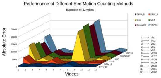
Figure 17.
Absolute omnidirectional error of six bee counting algorithms on twelve evaluation videos; VGG16 refers to MOG2/VG16; ResNet32 refers to MOG2/ResNet32; GS3 refers to MOG2/ConvNetGS3; GS4 refers to MOG2/ConvNetGS4.
Table 2.
PIV parameters used in absolute error comparison experiments.
4.5. Directional Bee Traffic
We cannot use our evaluation dataset for evaluating the directional bee counts of BeePIV (either with DPIV_A or DPIV_B), because we curated the videos for omnidirectional bee traffic (i.e., bee motions in any direction). Curating the videos for directional bee traffic would involve marking each detected bee motion in every frame as incoming, outgoing, and lateral, and specifying the angle of each motion with respect to a fixed coordinate system. We currently lack sufficient resources for this type of curation.
We can, however, use an indirect approach based on the hypothesis that in a typical hive the levels of incoming and outgoing bee traffic should match fairly closely over a given period of time, because all foragers (or most of them) that leave the hive eventually come back. If we consider the incoming and outgoing bee motion counts obtained with BeePIV as time series, we are likely to see that, in the long run, the incoming and outgoing series should follow each other fairly closely. Hives for which this is not the case may be failing or struggling.
We used the indirect approach outlined in the previous paragraph to estimate the performance of BeePIV (see Equation (31)) with DPIV_B (see Equation (35)) on all videos captured with the BeePi monitors deployed on the two beehives from May to November, 2018. Each BeePi monitor recorded a 30-s video every 15 min from 8:00 to 21:00. Thus, there were 4 videos every hour with a total 52 videos each day. We refer to these hives as R_4_5 and R_4_7 to describe and analyze our directional bee traffic experiments. Both hives were located in the same apiary in Logan, Utah ≈10 m apart. Although we had four monitored hives in that apiary, we chose to use the data from R_4_5 and R_4_7, because the BeePi monitors on these hives had the least number of hardware failures during the 2018 beekeeping season (May–November, 2018). R_4_5 was in sunlight from early morning until 12:00; R_4_7 remained in the shade most of the day and received sunlight from 16:30 to 18:30.
In our first experiment, we randomly chose 2 days from each month from May to August, 2018 (most active period in terms of bee traffic) from R_4_5 and R_4_7 to compute the incoming and outgoing bee motion count curves and to see how closely they follow each other. Our dataset included 832 videos from both hives. We applied BeePIV with DPIV_B to each video to obtain the counts of incoming and outgoing bee motions (i.e., and ). We henceforth refer to these curves as hourly bee motion count curves or as hourly curves. Figure 18 show the hourly curves for R_4_5 and R_4_7 for three different days in the chosen time period. While the overall shapes of the curves from the two hives are different, the incoming and outgoing curves of each hive closely follow each other. We also used Dynamic Time Warping (DTW) [28] to calculate the similarity between the incoming and outgoing time series. Lower DTW scores suggest the two curves are more closely aligned. Table 3 shows the DTW coefficients for the curves of the days in Figure 18 and several additional days.
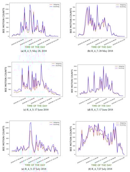
Figure 18.
Incoming and outgoing bee motion count curves for hives R_4_5 and R_4_7 on three different days in 2018; x-axis denotes time of day of video recording; y-axis denotes hourly means of incoming and outgoing traffic for corresponding hours.
Table 3.
DTW scores between outgoing and incoming curves in Figure 18 and several other days in 2018 beekeeping season; lower DTW values reflect closer curve alignments.
We computed the hourly incoming and outgoing curves for both hives for all the days in June–August, 2018. Figure 19 show the computed curves. Table 4 gives the mean daily DTW scores between the curves for June, July, and August, 2018 for both hives.
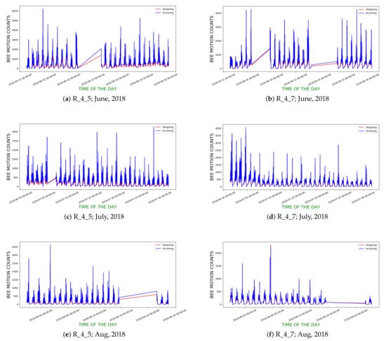
Figure 19.
Hourly incoming and outgoing bee motion curves of R_4_5 and R_4_7 in June, July and August 2018; straight line segments in curves indicate lack of data on corresponding periods due to hardware failures.
Table 4.
Mean daily DTW between hourly outgoing and incoming curves in June, July and August, 2018.
The plots and low DTW scores indicate that the incoming and outgoing bee traffic patterns appear to follow each other closely. We observed occasional spikes in incoming traffic that were not matched by similar spikes in outgoing traffic. On a closer examination of the corresponding videos, we observed that some bees were flying in and out too fast for the DPIV_B method to detect corresponding displacement vectors with an ordinary raspberry pi camera with a frame rate of 25 frames per second. In fact, we could barely detect some of these motions ourselves.
4.6. Directional Bee Traffic as Predictor of Colony Failure
The ultimate objective of an EBM system such as BeePi is to predict problems with monitored honeybee colonies. Since we knew from our manual beekeeper’s log that R_4_7 died in January 2019 whereas R_4_5 survived the winter and thrived in 2019, we inspected the incoming and outgoing curves for both hives from May to November 2018 for possible signs of failure. To compare the bee traffic in the two hives, we computed the mean of the incoming and outgoing bee motion counts for each day in the period from May to November, 2018 and plotted the incoming and outgoing curves for each hive. Figure 20 shows the two curves for this time period.
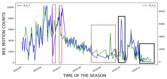
Figure 20.
Bee motion counts for the entire season of 2018; red boxes signify time periods with lack of data due to hardware failures in either hive.
To interpret the plots in Figure 20, one must discard the straight segments of the curves marked with red boxes, because they signify periods with no data from either hive due to hardware failures in our monitors that we had to fix before re-deploying them. The other parts of the curves indicate that the hives R_4_5 and R_4_7 were performing on par until November, 2018 when R_4_5 (the green curve) outperformed R_4_7 (the blue curve) for approximately three weeks.
We observed two important bee traffic events in the curves and marked them with two black boxes in Figure 20. The first black box above the value 2018-10 on the x-axis shows that there was a sudden increase in incoming and outgoing bee traffic in hive R_4_7, which we could not explain after we watched the real videos from that period and read our beekeeping log entries for that period.
The second black box above the value 2018-11 on the x-axis is more revealing. The curves in the box correspond to the period from the end of October 2018 to the end of November 2018, when the temperature becomes lower, which explains lower traffic in both hives. However, the higher variability of the R_4_5 green curve indicates that the bees in that hive were still flying in and out. On the other hand, the blue traffic curve for R_4_7 exhibits almost no variability and is consistently below the R_4_5 green curve, which indicates that the hive was in a weaker health condition. Indeed, our beekeeping log entries for R_4_7 show that it had fewer bees and less honey stored for the winter than R_4_7, which may account for the hive’s colony death approximately two months later.
4.7. Testing BeePIV on Raspberry Pi Platform
As we have stated in our previous articles (e.g., [7]), a long-term objective of the BeePi project is to develop an open citizen science platform for researchers, practitioners, and citizen scientists worldwide who want to monitor beehives. One of the essential characteristics of a citizen science platform is scalability. Thus, it is essential to ask the question of how much physical time the BeePIV algorithm takes when executed on the raspberry pi computer functioning as the computational unit of a deployed BeePi monitor. Since a BeePi monitor, records a 30-s video every 15 min, we can re-formulate our question in a more precise fashion: Can BeePIV, when executed on the raspberry pi computer, provide the bee motion counts for a given video before the next video is taken?
To answer this question, we executed BeePIV with DPIV_B on the 32 videos in the testbed and evaluation datasets on a raspberry pi 3 model B v1.2 with four cores, the model running in most of our currently deployed BeePi monitors. Table 5 shows the actual physical time taken by BeePIV to process each video on this raspberry pi platform. The results indicate that the processing time varies from video to video. In seconds, the mean processing time is 128.90 with a standard deviation of 61.68; in minutes, the mean processing time is 2.15 with a standard deviation of 1.03. While the longest time of 5.87 min taken by BeePIV on video 32 is significantly higher than the mean, it is significantly lower than 15 min (i.e., the length of the interval in between consecutive videos taken by the BeePi monitor). Hence, our test indicates that BeePIV can be used in situ to process bee traffic videos captured by deployed BeePi monitors.
Table 5.
Physical processing times for each video in our testbed and evaluation datasets; counts in columns Human Count and BeePIV Count are omnidirectional.
5. Summary
In this article, we have presented BeePIV, a video-based algorithm for measuring omnidirectional and directional honeybee traffic. The algorithm is a new significant result in our ongoing longitudinal investigation of honeybee flight and traffic in images and videos acquired with our deployed BeePi EBM systems. BeePIV converts frames from bee traffic videos to particle motion frames with uniform white background, applies PIV to these motion frames to compute particle displacement vector fields, classifies individual displacement vectors as incoming, outgoing, and lateral, and uses vector counts to measure incoming, outgoing, and lateral bee traffic.
We postulated the existence of functions that map color variation to video-specific threshold and distance values that can be used to reduce smoothed difference frames to uniform background frames with motion points and defined and evaluated two such functions. Our experiments with using those functions in BeePIV partially verified our conjecture that thresholds and distances can be obtained from video color variation insomuch as BeePIV outperformed our previously implemented omnidirectional bee counting methods on twelve manually curated bee traffic videos. We readily acknowledge that these results are suggestive in nature and that more curated videos are needed for experimentation. We currently lack sufficient resources to execute this curation, because curating videos for directional bee traffic involves marking each detected bee motion in every frame as incoming, outgoing, and lateral and specifying the angle of each motion with respect to a fixed coordinate system. We plan to perform this curation in the future on the videos in the testbed and evaluation datasets.
We proposed an indirect method to evaluate incoming and outgoing traffic based on the hypothesis that in many hives the levels of incoming and outgoing traffic should match fairly closely over a given period of time. The bee motion curves we computed for two hives indicate that the incoming and outgoing bee traffic patterns closely follow each other. We experimentally observed that in the healthy hive R_4_5 there was a period of time when the bees were flying in and out whereas in the failing hive R_4_7 the traffic curve over the same period exhibited almost no variability and was consistently below the curve of the healthy hive. We also observed that the hourly bee motion curves followed each other closely in the failing hive, too.
Our experiments with estimating the physical run times of BeePIV on the raspberry pi platform showed that the algorithm can be used in situ to process bee traffic videos in deployed BeePi monitors. In seconds, the mean processing time of executing BeePIV on the raspberry pi 3 model B v1.2 with four cores on 32 videos in our testbed and evaluation datasets was 128.90 with a standard deviation of 61.68; in minutes, the mean processing time on the same videos was 2.15 with a standard deviation of 1.03. While the longest time of 5.87 min taken by BeePIV on video 32 was significantly higher than the mean time, it was significantly lower than 15 min (i.e., the length of the interval in between consecutive videos taken by the BeePi monitor).
Supplementary Materials
The following are available online at https://www.mdpi.com/2076-3417/11/5/2276/s1.
Author Contributions
Supervision, Project Administration, and Resources, V.K., A.M.; Conceptualization and Software, S.M., V.K., T.T.; Data Curation, V.K., S.M.; Writing—Original Draft Preparation, V.K., S.M. Writing—Review and Editing, V.K., S.M., A.M.; Investigation and Analysis, S.M., V.K.; Validation, S.M., V.K. All authors have read and agreed to the published version of the manuscript.
Funding
This research is funded, in part, by our Kickstarter research fundraisers in 2017 [23] and 2019 [24]. This research is based, in part, upon work supported by the U.S. Office of Naval Research Navy and Marine Corps Science, Technology, Engineering and Mathematics (STEM) Education, Outreach and Workforce Program, Grant Number: N000141812770. Any opinion, findings, conclusions, or recommendations expressed in this material are those of the authors and do not necessarily reflect the views of the sponsor.
Data Availability Statement
Since we lack the resources to host the testbed and evaluation datasets online permanently, interested readers are encouraged to make individual email arrangements with the first author in case they want to obtain these datasets.
Acknowledgments
We would like to thank all our Kickstarter backers and especially our BeePi Angel Backers (in alphabetical order): Prakhar Amlathe, Ashwani Chahal, Trevor Landeen, Felipe Queiroz, Dinis Quelhas, Tharun Tej Tammineni, and Tanwir Zaman. We express our gratitude to Gregg Lind, who backed both fundraisers and donated hardware to the BeePi project. We are grateful to Richard Waggstaff, Craig Huntzinger, and Richard Mueller for letting us use their property in northern Utah for longitudinal EBM tests. We would like to thank Anastasiia Tkachenko for many valuable suggestions during the revision of this manuscript.
Conflicts of Interest
The authors declare no conflict of interest.
Abbreviations
The following abbreviations are used in this manuscript:
| EBM | Electronic Beehive Monitoring |
| FFT | Fast Fourier Transform |
| PIV | Particle Image Velocimetry |
| DPIV | Digital Particle Image Velocimetry |
| OpenPIV | Open Particle Image Velocimetry |
| JPIV | Java Particle Image Velocimetry |
| OpenCV | Open Computer Vision |
| DTW | Dynamic Time Warping |
| ConvNet | Convolutional Network |
| CSV | Comma Separated Values |
References
- Winston, M. The Biology of the Honey Bee; Harvard University Press: Cambridge, MA, USA, 1987. [Google Scholar]
- Page, R., Jr. The spirit of the hive and how a superorganism evolves. In Honeybee Neurobiology and Behavior: A Tribute to Randolf Menzel; Galizia, C.G., Eisenhardt, D., Giurfa, M., Eds.; Springer: Berlin, Germany, 2012; pp. 3–16. [Google Scholar] [CrossRef]
- Ferrari, S.; Silva, M.; Guarino, M.; Berckmans, D. Monitoring of swarming sounds in bee Hives for early detection of the swarming period. Comput. Electron. Agric. 2008, 64, 72–77. [Google Scholar] [CrossRef]
- Meikle, W.G.; Holst, N.; Mercadier, G.; Derouan, F.; James, R.R. Using balances linked to dataloggers to monitor honey bee colonies. J. Apic. Res. 2006, 45, 39–41. [Google Scholar] [CrossRef]
- Mukherjee, S.; Kulyukin, V. Application of digital particle image velocimetry to insect motion: Measurement of incoming, outgoing, and lateral honeybee traffic. Appl. Sci. 2020, 10, 2042. [Google Scholar] [CrossRef]
- Langstroth Beehive. Available online: https://en.wikipedia.org/wiki/Langstroth_hive (accessed on 7 January 2021).
- Kulyukin, V.; Mukherjee, S. On video analysis of omnidirectional bee traffic: Counting bee motions with motion detection and image classification. Appl. Sci. 2019, 9, 3743. [Google Scholar] [CrossRef]
- Kulyukin, V.; Putnam, M.; Reka, S. Digitizing buzzing signals into A440 piano note sequences and estimating forager traffic levels from images in solar-powered, electronic beehive monitoring. In Lecture Notes in Engineering and Computer Science, Proceedings of the International MultiConference of Engineers and Computer Scientists; Newswood Limited: Hong Kong, China, 2016; Volume 1, pp. 82–87. [Google Scholar]
- Kulyukin, V.; Reka, S. Toward sustainable electronic beehive monitoring: Algorithms for omnidirectional bee counting from images and harmonic analysis of buzzing signals. Eng. Lett. 2016, 24, 317–327. [Google Scholar]
- Willert, C.E.; Gharib, M. Digital particle image velocimetry. Exp. Fluids 1991, 10, 181–193. [Google Scholar] [CrossRef]
- Adrian, R.J. Particle-imaging techniques for experimental fluid mechanics. Annu. Rev. Fluid Mech. 1991, 23, 261–304. [Google Scholar] [CrossRef]
- Dickinson, M.; Lehmann, F.; Sane, S. Wing rotation and the aerodynamic basis of insect flight. Science 1999, 284, 1954–1960. [Google Scholar] [CrossRef]
- Bomphrey, R.J.; Lawson, N.J.; Taylor, G.K.; Thomas, A.L.R. Application of digital particle image velocimetry to insect aerodynamics: Measurement of the leading-edge vortex and near wake of a hawkmoth. Exp. Fluids 2006, 40, 546–554. [Google Scholar] [CrossRef]
- Michelsen, A. How do honey bees obtain information about direction by following dances? In Honeybee Neurobiology and Behavior: A Tribute to Randolf Menzel; Galizia, C., Eisenhardt, D., Giurfa, M., Eds.; Springer: Berlin, Germany, 2012; pp. 65–76. [Google Scholar] [CrossRef]
- Rodriguez, I.F.; Megret, R.; Egnor, R.; Branson, K.; Agosto, J.L.; Giray, T.; Acuna, E. Multiple insect and animal tracking in video using part affinity fields. In Proceedings of the Workshop Visual Observation and Analysis of Vertebrate and Insect Behavior (VAIB) at International Conference on Pattern Recognition (ICPR), Beijing, China, 20–24 August 2018. [Google Scholar]
- Babic, Z.; Pilipovic, R.; Risojevic, V.; Mirjanic, G. Pollen bearing honey bee detection in hive entrance video recorded by remote embedded system for pollination monitoring. ISPRS Ann. Photogramm. Remote Sens. Spat. Inf. Sci. 2016, 3, 51–57. [Google Scholar] [CrossRef]
- Minichiello, A.; Armijo, D.; Mukherjee, S.; Caldwell, L.; Kulyukin, V.; Truscott, T.; Elliott, J.; Bhouraskar, A. Developing a mobile application-based particle image velocimetry tool for enhanced teaching and learning in fluid mechanics: A design-based research approach. Comput. Appl. Eng. Educ. 2020, 1–21. [Google Scholar] [CrossRef]
- Armijo, D. Benchmarking of a Mobile Phone Particle Image Velocimetry System. Master’s Thesis, Department of Mechanical and Aerospace Engineering, Utah State University, Logan, UT, USA, 2020. [Google Scholar]
- OpenPIV. Available online: http://www.openpiv.net/ (accessed on 7 January 2021).
- JPIV. Available online: https://github.com/eguvep/jpiv/ (accessed on 7 January 2021).
- PIVLab. Available online: https://github.com/Shrediquette/PIVlab/releases/tag/2.38 (accessed on 7 January 2021).
- Kulyukin, V.; Mukherjee, S.; Amlathe, P. Toward audio beehive monitoring: Deep learning vs. standard machine learning in classifying beehive audio samples. Appl. Sci. 2018, 8, 1573. [Google Scholar] [CrossRef]
- Kulyukin, V. BeePi: A Multisensor Electronic Beehive Monitor. Available online: https://www.kickstarter.com/projects/970162847/beepi-a-multisensor-electronic-beehive-monitor (accessed on 7 January 2021).
- Kulyukin, V. BeePi: Honeybees Meet AI: Stage 2. Available online: https://www.kickstarter.com/projects/beepihoneybeesmeetai/beepi-honeybees-meet-ai-stage-2 (accessed on 7 January 2021).
- Zivkovic, Z. Improved adaptive gaussian mixture model for background subtraction. In Proceedings of the 17th international conference on pattern recognition (ICPR), Cambridge, UK, 26–26 August 2004; Volume 2, pp. 28–31. [Google Scholar]
- KaewTraKulPong, P.; Bowden, R. An Improved adaptive background mixture model for real-time tracking with shadow detection. In Proceedings of the Second European Workshop on Advanced Video Based Surveillance Systems (AVBS01), Kingston, UK, September 2001; pp. 28–31. [Google Scholar] [CrossRef]
- Zivkovic, Z.; van der Heijden, F. Efficient adaptive density estimation per imge pixel for the task of background subtraction. Pattern Recognit. Lett. 2006, 27, 773–780. [Google Scholar] [CrossRef]
- Salvador, S.; Chan, P. Toward accurate dynamic time warping in linear time and space. Intell. Data Anal. 2007, 11, 561–580. [Google Scholar] [CrossRef]


Publisher’s Note: MDPI stays neutral with regard to jurisdictional claims in published maps and institutional affiliations. |
© 2021 by the authors. Licensee MDPI, Basel, Switzerland. This article is an open access article distributed under the terms and conditions of the Creative Commons Attribution (CC BY) license (http://creativecommons.org/licenses/by/4.0/).