Article

Study on Accuracy Metrics for Evaluating the Predictions of Damage Locations in Deep Piles Using Artificial Neural Networks with Acoustic Emission Data

1
School of Resource & Civil Engineering, Northeastern University, Shenyang 110819, China
2
Department of Civil and Environmental Engineering, Pusan National University, Busan 46241, Korea
*
Authors to whom correspondence should be addressed.
Appl. Sci. 2021, 11(5), 2314; https://doi.org/10.3390/app11052314
Submission received: 29 January 2021 / Revised: 24 February 2021 / Accepted: 1 March 2021 / Published: 5 March 2021

Abstract

:
Accuracy metrics have been widely used for the evaluation of predictions in machine learning. However, the selection of an appropriate accuracy metric for the evaluation of a specific prediction has not yet been specified. In this study, seven of the most used accuracy metrics in machine learning were summarized, and both their advantages and disadvantages were studied. To achieve this, the acoustic emission data of damage locations were collected from a pile hit test. A backpropagation artificial neural network prediction model for damage locations was trained with acoustic emission data using six different training algorithms, and the prediction accuracies of six algorithms were evaluated using seven different accuracy metrics. Test results showed that the training algorithm of “TRAINGLM” exhibited the best performance for predicting damage locations in deep piles. Subsequently, the artificial neural networks were trained using three different datasets collected from three acoustic emission sensor groups, and the prediction accuracies of three models were evaluated with the seven different accuracy metrics. The test results showed that the dataset collected from the pile body-installed sensors group exhibited the highest accuracy for predicting damage locations in deep piles. Subsequently, the correlations between the seven accuracy metrics and the sensitivity of each accuracy metrics were discussed based on the analysis results. Eventually, a novel selection method for an appropriate accuracy metric to evaluate the accuracy of specific predictions was proposed. This novel method is useful to select an appropriate accuracy metric for wide predictions, especially in the engineering field.

1. Introduction

To transform the load from superstructures to the hard stratum, pile foundations have been widely designed in the construction of modern structures [1,2,3,4]. The stability of structures mostly relies on the health situations of the pile foundations. Due to its importance, the health monitoring of pile foundations is always of special interest in engineering [5]. As a passive non-destructive testing (NDT) technique, acoustic emission (AE) has been successfully used for the health monitoring of pile foundations [6,7]. An advantage of AE techniques is that in-service structures can be monitored continually without any disturbance [8,9]. The detection of damage locations using the AE technique is an important research topic in NDT studies.
AE refers to the elastic waves generated from the cracks in a failed material [10]. When failure occurs, elastic waves propagate inside the material and can be received by the AE sensors installed on the outer faces of the material [6,11]. The elastic waves are collected by the AE data acquisition system and processed to detect the damage locations or evaluate the damage degree of the material [12].
Several applications of AE technique for detecting damages to concrete piles have been studied in recent years. William et al. [3] conducted an experimental study to recognize and classify corrosion damage in concrete piles using an AE detection technique. Mao et al. [5] studied the AE characteristics of failure process and discussed the feasibility of using AE for the damage monitoring of shallow pile foundations. Len et al. [13] proposed a wave propagation-based NDT technology for deep concrete piles.
Artificial neural networks (ANNs) are one of the most popular machine learning algorithms that simulate the human brain’s neural networks in terms of information processing [14,15,16]. ANNs are computational systems that are connected by a large number of elements [15]. ANNs have a strong ability to reveal the unknown relations between variables and predict the probable output by training the given variables [17]. ANNs have been successfully applied in the engineering field and have shown good intelligence ability [14]. Over the recent years, several applications of ANNs for predicting damage locations on plate-like structures have been reported [18,19,20]. However, the application of ANNs for predicting damage locations on real structures (three-dimensional structures) such as pile foundations has not yet been reported. Moreover, how to evaluate the prediction accuracy of damage locations using ANNs for real structures is another urgent issue.
Accuracy metrics in ANNs are used to evaluate the goodness of predictions. Mean square error (MSE), root mean square error (RMSE), mean absolute error (MAE), mean absolute percentage error (MAPE) and symmetric mean absolute percentage error (SMAPE) are the most popularly used accuracy metrics for the evaluation of ANN prediction models in the weather forecasting, medical and engineering fields [21,22,23,24,25,26,27].
However, different accuracy metrics are based on different types of measurements. For example, the calculations of MSE, RMSE and MAE are based on squared errors and absolute errors. The calculations of MAPE and SMAPE are based on percentage errors. Different accuracy metrics show different kinds of goodness. As different accuracy metrics have their own advantages and disadvantages, for a specific prediction model, some accuracy metrics may not be appropriate. Thus, the selection of an appropriate accuracy metric to evaluate ANN prediction models is a very important issue.
The purpose of this research was to build an ANN prediction model for damage locations of deep piles and propose a novel selection method for an appropriate metric to evaluate the accuracy of predictions. A step-by-step block diagram of the proposed research is presented in Figure 1. The research was composed of four steps: in step 1, the commonly used accuracy metrics were classified and summarized based on their calculation measures, and both the advantages and disadvantages of the accuracy metrics were illustrated; in step 2, a pile hit experiment was conducted to collect the experimental data to train the ANN prediction model, and then an ANN prediction model was developed to predict the damage locations; in step 3, prediction results of the ANN model were analyzed and evaluated using accuracy metrics; finally, in step 4, the correlations and sensitivity of the accuracy metrics were discussed, and a novel selection method for an appropriate accuracy metric was proposed.

2. Accuracy Metrics

2.1. Correlation-Based Metrics

The correlation coefficient (R) and coefficient of determination (R2) are widely used for the evaluation of the goodness of linear fit of regression models in ANNs [28]. Pearson correlation coefficient, Spearman’s rank correlation coefficient and Kendall rank correlation coefficient are commonly used correlation coefficients in statistics. The R refer to the Pearson correlation coefficient in this study. The R interprets the degree of correlation between the actual and predicted variables [29,30]. The calculation of R is illustrated in the Equation (1), the numerator is the sum of squares of residuals also called the residual sum of squares, and the denominator is the total sum of squares that is proportional to the variance of the data.
The magnitude of R ranges from −1 to +1 [31]. The strength of correlation of two variables can be described in five degrees, as illustrated in Figure 2. A value of +1 (or −1) indicates the perfect correlation between two variables, +1 is positive correlation and −1 is inverse correlation between two variables; a range from 0.8 to 1 (or from −0.8 to −1) indicates very strong correlation; a range from 0.6 to 0.8 (or from −0.6 to −0.8) indicates strong correlation; a range from 0.4 to 0.6 (or from −0.4 to −0.6) indicates moderate correlation; a range from 0.2 to 0.4 (or from −0.2 to −0.4) indicates week correlation; and a range from 0 to 0.2 (or from 0 to −0.2) indicates very week correlation.
The R2 is the ratio of the predicted variable that is explained by a regression model [32]. In other word, it is the ratio of explained variable from the total variable. R2 is the square of correlation between the actual variable and predicted variable [33]. Thus, R2 ranges from 0 to 1. A value of 0 indicates that the regression model explains none of the predicted variable, which means that there is no correlation between the two variables. A value of 1 indicates that the regression model explains all of the predicted variables, which means the that the correlation between the two variables is perfect. The explanations of other values between 0 and 1 can be found in Figure 2.
The calculation of R and R2 are defined as [28,29,30,31,32,33]
R = 1 n 1 n ( D act - D ¯ act ) ( D pre - D ¯ pre ) 1 n 1 n ( D act D ¯ act ) 2 1 n 1 n ( D pre D ¯ pre ) 2
R 2 = 1 1 n ( D act D pre ) 2 1 n ( D act D ¯ act ) 2
where D act is the actual variable, D pre is the predicted variable, D ¯ act is the mean value of the actual variable, D ¯ pre is the mean value of the predicted variable and n is the amount of collected data; variables refer to the distance from ground level in this case study.

2.2. Scale-Dependent Metrics

Metrics based on absolute errors or on squared errors are called scale-dependent metrics [34]. The scale-dependent metrics have the same scale as the original data [34] and provide errors in the same units [35]. However, the scale-dependent metrics can be difficult to compare for series that are on different scales or that have different units. For example, if a prediction error is 10 units, the gravity of the error cannot be evaluated unless the level of gravity is also provided [36].
Although the scale-dependent metrics are not unit-free, they are favored in machine learning evaluation. The commonly used scale-dependent metrics are MSE, RMSE and MAE. The calculation methods of the three metrics are defined as [37]
MSE = 1 n 1 n ( D pre D act ) 2
RMSE = 1 n 1 n ( D pre D act ) 2
MAE = 1 n 1 n | D pre D act |
MSE measures the mean squared error between the predicted value and actual value. For every data point, the distance is measured vertically from the actual value to the corresponding predicted value on the fit line, and the value is squared. Subsequently, the sum of all the squared values is calculated and divided by the number of points. Therefore, the unit of MSE is the square of the original unit. Due to the squaring of errors, the negative values and positive values do not cancel each other out.
The range of MSE is ( 0 , + ) ; the smaller the MSE value is, the higher the accuracy of the prediction model. The perfect value of MSE is 0, indicating that the prediction model is perfect. MSE is defaulted as the loss function of linear regression in machine learning.
RMSE measures the average magnitude of error between the predicted value and actual value. Thus, RMSE is the average distance measured vertically from the actual value to the corresponding predicted value on the fit line. Simply, it is the square root of MSE.
In the same manner as MSE, the range of RMSE is (0, + ) ; the smaller the RMSE value is, the higher the accuracy of the prediction model. In contrast with MSE, the units of RMSE are the same as original units, making the RMSE more interpretable than MSE.
MAE is a metric used to measure the average magnitude of the absolute errors between the predicted value and actual value. The MAE is often called the mean absolute deviation (MAD) [35,36,38]. The range of MAE is (0, + ); the smaller the MAE value is, the higher the accuracy of the prediction model. The advantage of MAE is that the unit of MAE is the same as original data, and it is easy to calculate and understand. The MAE is often used as a symmetrical loss function [36].
Both MAE and RMSE express the average magnitude of prediction error with the units of the original data. In comparison with MAE, the RMSE has a relatively high weight for large errors, because the errors are squared before averaging. If prediction errors are normally distributed, the MAE and RMSE can be switched with each other with Equation (6), which is defined as [35,36]
RMSE = 0.8 MAE
In summary, the scale-dependent metrics MSE, RMS, and MAE penalize errors according to their magnitude [35]. The disadvantage of these three metrics is that they are not unit-free, and it is difficult to compare predictions with different units. Moreover, MSE, RMSE and MAE interpret only the magnitude of error, but do not indicate the direction of error [38].

2.3. Percentage-Dependent Metrics

To compare predictions with different units, unit-free measures are needed. Since there is no limitation on units, percentage-dependent metrics are preferred for this issue. The percentage-dependent metrics measure the size of errors in percentage terms and provide interpretable thinking regarding the quality of prediction [36]. Interpretable thinking should be expressed in percentage terms when the scale of data is unknown. For instance, a report saying that “the prediction error is 5%” is more meaningful than saying “the prediction error is 50 cm (or other terms)”, if the reviewer does not know the scale of the data.
The most commonly used percentage-dependent metrics are MAPE and SMAPE [39], and they are defined as [35]
MAPE = 100 % n i = 1 n | D pre D act D act |
SMAPE = 100 % n i = 1 n | D pre D act ( | D pre | + | D act | ) / 2 |
The MAPE calculates the average of the percentage error. It is a measure of prediction accuracy, especially in trend estimation. The MAPE is also abbreviated as MAPD (“D” for “deviation”). The MAPE is used as the loss function for regression models in machine learning, since it is very intuitive to explain the relative error. The disadvantage of the MAPE is that the MAPE is scale-sensitive; it will get extreme values if the actual value is quite small. Thus, the MAPE should be avoided as an evaluation metric for low-scale data.
Another disadvantage of the MAPE is that it penalizes positive errors more heavily than negative errors [34,35,39]. For example, if the actual value of an original data point is 10, and its prediction value is 15, then the error is 5 (positive). The value of MAPE would be
MAPE = 100 % × | 15 10 10 | = 50 %
However, when the actual value is 15, and the prediction value is 10, then the error is still 5 (negative). The value of MAPE is much lower:
MAPE = 100 % × | 10 15 15 | = 33.33 %
The SMAPE is another commonly used percentage-dependent metric. It is the optimized version of MAPE. The SMAPE is regarded as the “symmetric” MAPE [34]. The SMAPE places the same penalty on both positive error and negative error.
However, if the actual value is zero, and the prediction value is also zero or close to zero, the value of SMAPE is likely to be infinite [34]. Another disadvantage of SMAPE is that it is much more complex to calculate than other metrics.
The range of both MAPE and SMAPE is (0%, + ); the smaller the value of MAPE and SMAPE, the better the accuracy of the prediction model. The perfect value of MAPE and SMAPE is 0%, indicating that the prediction model is perfect. If the value of MAPE and SMAPE is greater than 100%, this indicates that the prediction model is very poor.

3. Damage Location Prediction Model Using AE Signal Data

3.1. Experimental Setup of Pile Hit Test

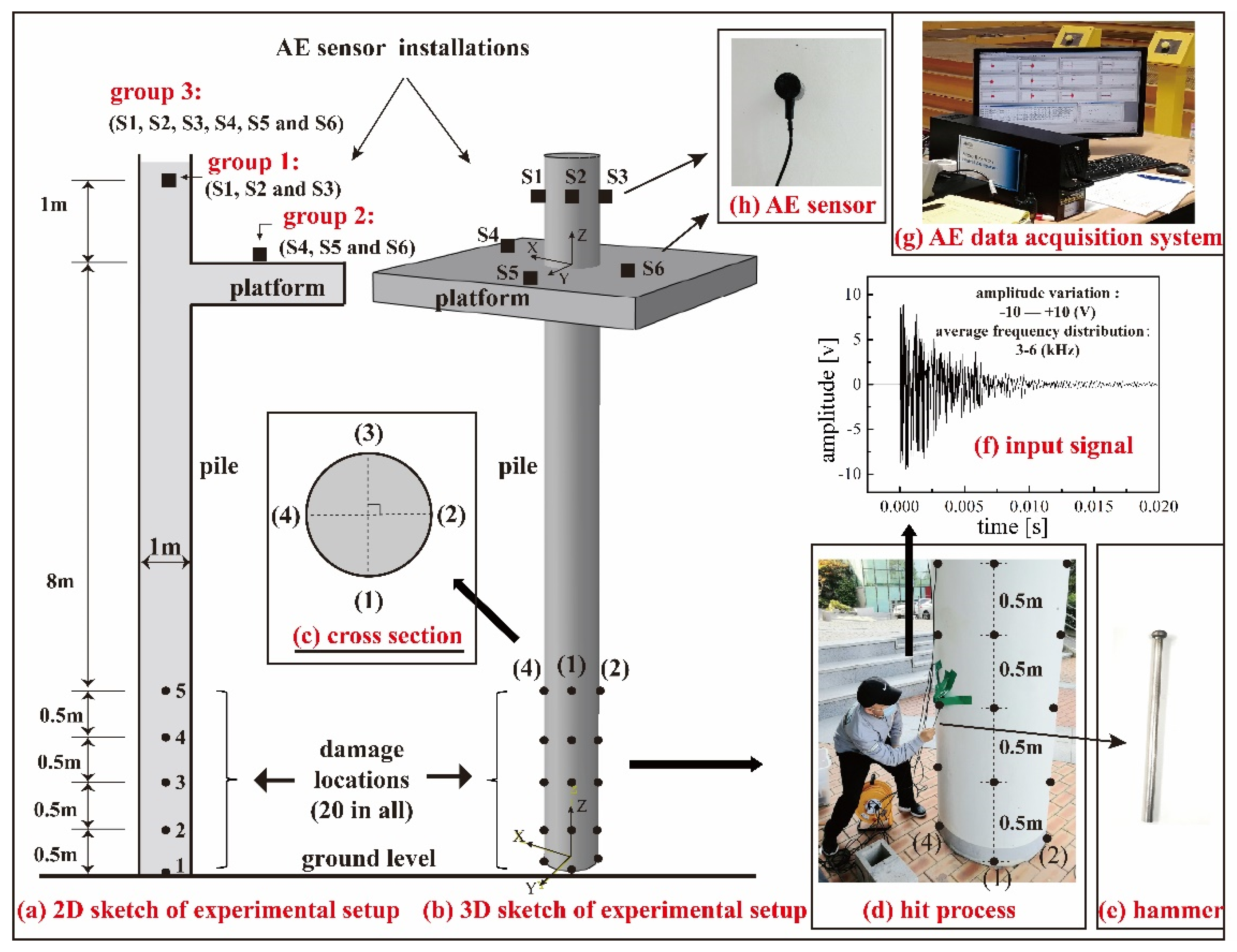
A pile hit test was conducted to collect the experimental data for the ANN prediction model. The experimental setup of the pile hit test is illustrated in Figure 2. A circular section concrete column of a building was determined as the test specimen. This concrete column represented a deep pile, since the concrete column and pile shared the same structure and components. The height of the test pile was 11 m, and the diameter of the pile was 1 m. A platform was connected to the pile at the height of 10 m from ground level.
It was more difficult to detect the damage of deep piles compared to upper structures, as the piles were always hidden in soil. When detecting the damage of deep piles, how to install the sensors for receiving signal was always a confusing problem for engineers. There were three main methods for installing the sensors: installing the sensors on pile body, installing the sensors on platform, and installing sensors on both pile body and platform (mix-installation). However, the efficiency of the three installation methods for detecting the damage in a deep pile were need to be studied.
In this experiment, six AE sensors were installed on the pile body and platform. In which, three AE sensors were installed on the pile body at the height of 11 m from the ground level on three perpendicular sides. The three AE sensors were marked as S1, S2 and S3, and they were classified in group 1. The group 1 was named as pile-installed group. Another three AE sensors were installed on the platform on three perpendicular sides corresponding to the pile-installed sensors. The three AE sensors were marked as S4, S5 and S6, and they were classified in group 2. The group 2 was named as plate-installed group. For the group 3, the AE sensors of the group 1 and group 2 were combined together as a mix-installed group. Thus, there were six AE sensors in the group 3, they were S1, S2, S3, S4, S5, and S6 (Figure 3a).
The experimental data were collected by a Micro-II; Digital AE system installed on the platform (Figure 3g). The threshold (trigger level for collecting AE signals) was set as 40 dB after pretesting, which can effectively prevent surrounding noise interference. The AE sensor type was R.45IC (Figure 3h), which was commonly selected for structural health monitoring of concrete structures. The operating specifications of R.45IC type AE sensor are shown in Table 1. AE sensors were installed on the pile and platform using high vacuum grease, which can help AE sensors to gather signals. The six AE sensors were connected to the AE system with cables and the AE system can output the AE signal data for users.

3.2. Data Collection of AE Signals

The damage was determined as the impact damage in this study. To generate the impact damages, the test pile was hit with a small iron hammer as illustrated in Figure 3d. Each hit point (damage location) was hit five times with a constant force. The waveforms of the input signals are shown in Figure 3f; the maximum amplitude was 10 V and the average frequency was 3–6 kHz. The vibration time is 0.02 s.
Five hit points were determined to generate AE signals of damage locations from ground level to the height of 2 m every 0.5 m on one side of the test pile. There were four perpendicular sides on this test pile (Figure 3c), and each side had five hit points. In total, there were 20 hit points on this test pile. Each point was hit five times with a constant strength, and five AE signals were generated corresponding to five hits. One hundred AE signals were generated in total, and all signals were received by six AE sensors; in other words, one AE sensor collected 100 AE signal’s data, and thus 600 AE signal’s data were collected by six AE sensors. According to the grouping of the AE sensors, there were 300 AE signals collected in group 1, 300 AE signals in group 2, and 600 AE signals in group 3, respectively.

3.3. ANN Prediction Model

The training of ANNs can be processed in a supervised or unsupervised manner [40]. An ANN model trained in supervised learning manner can output high accuracy prediction by given enough training data. Backpropagation ANNs are the most used supervised learning neural networks [17,41]. The strong nonlinear mapping ability is one of the excellent advantages of backpropagation ANNs [14]. In the backpropagation ANNs, the signals propagate forward and the errors propagate backward until the output value is acceptable [42].
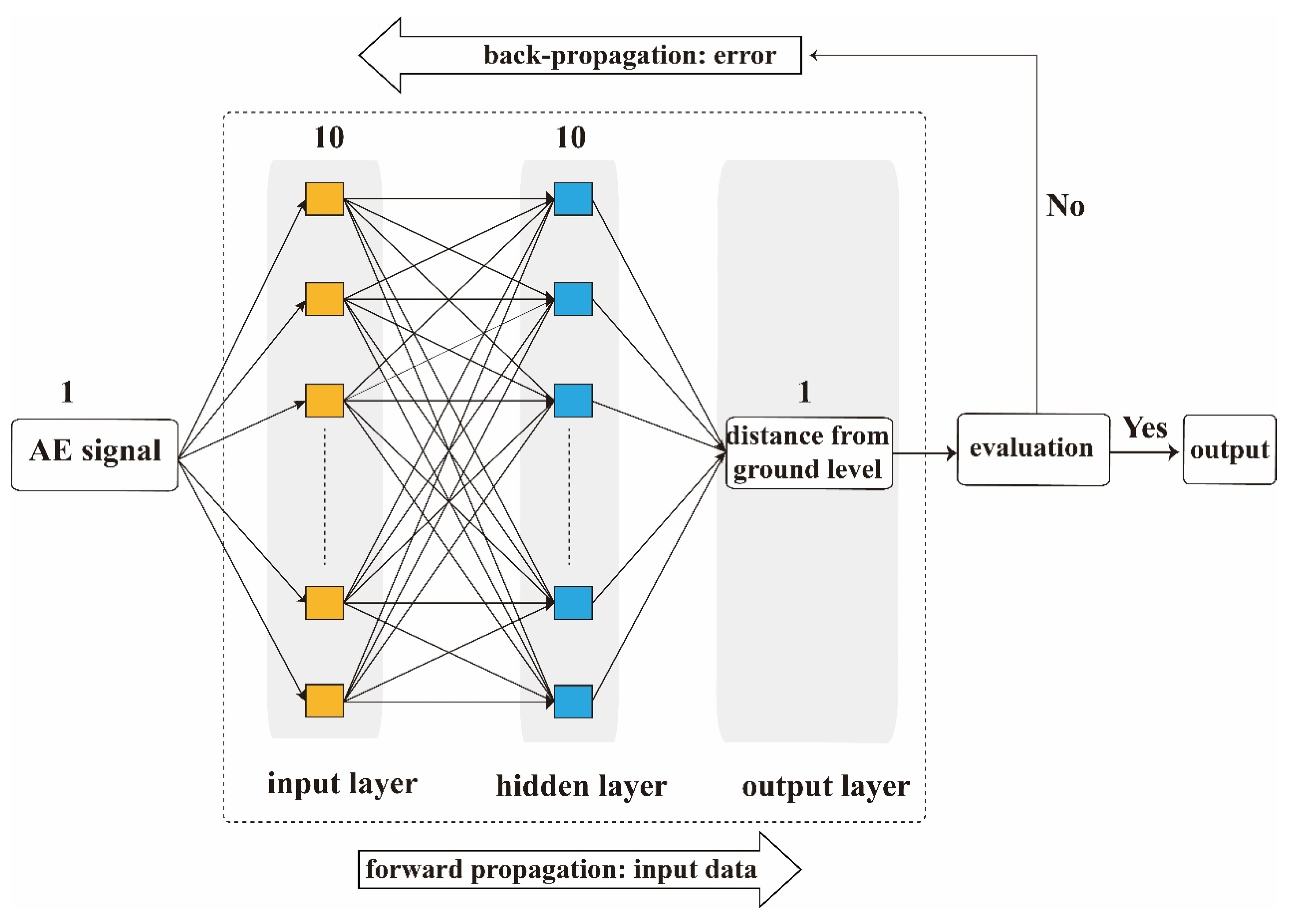
Figure 4 illustrates the schematic diagram of the backpropagation ANN prediction model for the damage locations. The backpropagation ANN prediction model is composed of one input layer, one hidden layer and one output layer. The number of hidden layers and quantity of neurons are determined through the training process until the prediction accuracy cannot be further improved [43]. However, one hidden layer is commonly used for simple predictions [43]. The quantity of neurons of input and output layers is equal to the number of input and output variables, respectively [44]. In the case of the backpropagation ANN prediction model in this study, the quantity of neurons of input and output layers was one, since there was only one variable. One hidden layer and ten neurons were determined for the backpropagation ANN prediction model after pretesting.
In the learning process of the backpropagation ANN prediction model, AE signals generated from the pile hit test were inputted from the input layer. Subsequently, the AE signals reached the output layer through the hidden layer. The damage locations were identified with the distance from ground level of each hit point at the output layer. The backpropagation ANN prediction model was trained using MATLAB 2020.

4. Evaluations of Prediction Results Using Accuracy Metrics

4.1. Evaluations of Performance of Different Training Algorithms

4.1.1. Evaluations of Performance Using Scale-Dependent Metrics

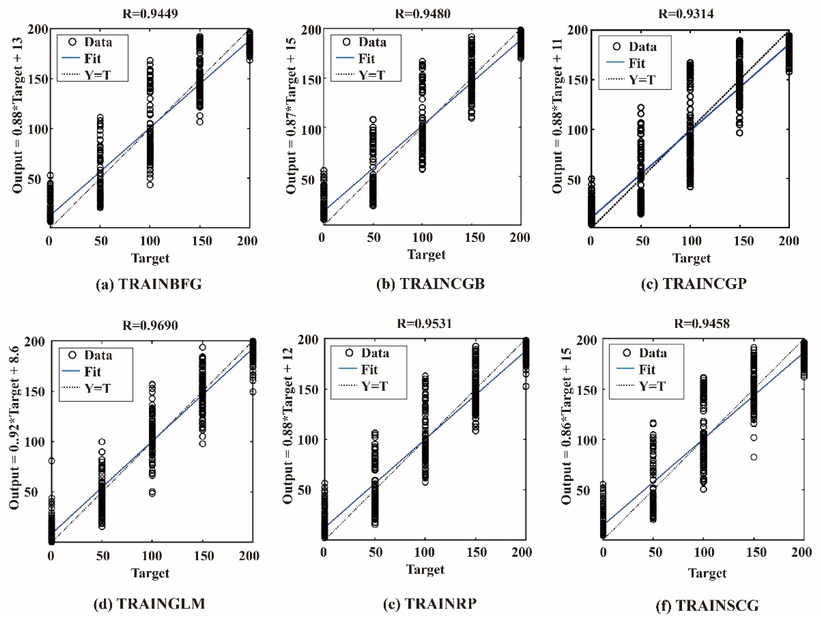
Figure 5 shows the regression plot of backpropagation ANN prediction models with the six network training algorithms as illustrated in Table 2 [45]. The ANN prediction model was trained using the 600 AE signal dataset. In Figure 5, the target values refer to the actual value of damage locations, while the output values refer to the prediction values of damage locations. The black circles represent the individual data points.
It can be observed from Figure 5 that the regression plots of the six algorithms were approximately the same, and it was difficult to evaluate the performance of the six algorithms. Thus, it is essential to compare the performance of different algorithms using accuracy metrics.
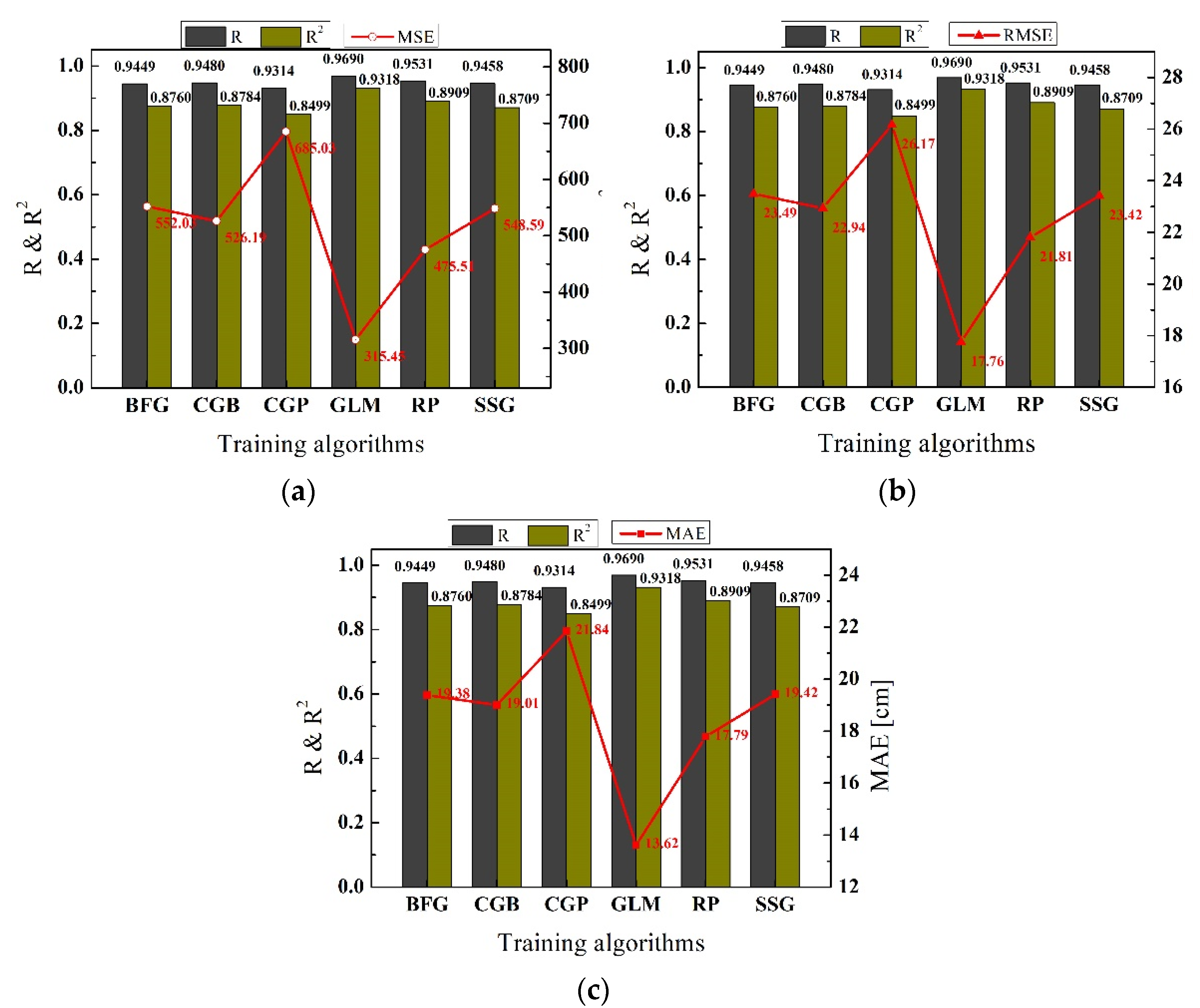
The evaluation results of the performance of six different training algorithms using scale-dependent metrics are shown in Table 3 and Figure 6. In Figure 6, the R and R2 are shown with columns to evaluate the goodness of linear fit for the regression model. The MSE, RMSE and MAE are shown with a variation curve to evaluate the errors of prediction.
The R value of the “TRAINGLM” algorithm was 0.9690, and it was the maximum of the six training algorithms. The R value of the “TRAINCGP” algorithm was 0.9314, and it was the minimum of the six training algorithms. According to the degree of correlations, as shown in Figure 2, all of the six regression models (prediction models) showed very strong correlations between the actual value and predicted value.
For the R2, the value of the “TRAINGLM” algorithm was 0.9318, and it was also the maximum of the six training algorithms. The R2 value of the “TRAINCGP” algorithm was 0.8499, and it was also the minimum of the six training algorithms. The R2 values of the six training algorithms were greater than 0.80, indicating that the regression models explained the predicted values very well.
The evaluation results of MSE, RMSE and MAE for the “TRAINGLM” algorithm were 315.45 cm2, 17.76 cm and 13.62 cm, respectively. They were the minima of the evaluation values of the six training algorithms. The evaluation values of MSE, RMSE and MAE for the “TRAINCGP” algorithm were 685.03 cm2, 26.17 cm and 21.84 cm, respectively, and they were the maxima of the evaluation values of the six training algorithms.
It can be inferred from the evaluation results of correlation metrics and scale-dependent metrics that the “TRAINGLM” algorithm shows the best performance for training the backpropagation ANN prediction model, and the “TRAINCGP” algorithm has the worst performance for training the backpropagation ANN prediction model of damage locations in deep piles.

4.1.2. Evaluations of Performance Using Percentage-Dependent Metrics

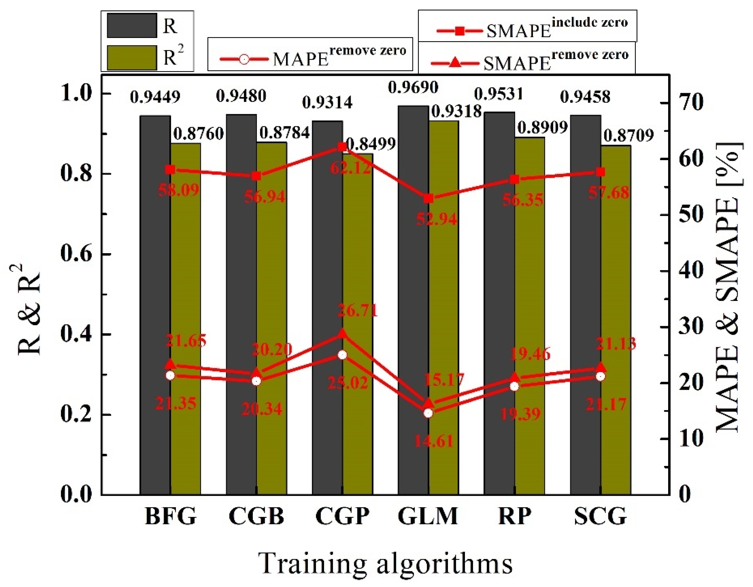
The evaluation results of the performance of the six different training algorithms using percentage-dependent metrics are shown in Table 4 and Figure 7. As there were zero values in the actual values of the prediction model, the calculation results of MAPE were infinite. The reason for this was that the actual values were denominators in the calculation algorithm of MAPE (refer to Equation (7)). To eliminate the influences of zero values on the calculation results, the MAPE scores were calculated after the zero values were removed from the actual values.
Calculation results of the MAPE without zero values are shown in Table 4. The evaluation result of the MAPE for the algorithm was 14.61%, and it was the minimum of the evaluation results of the six training algorithms. The evaluation result of MAPE for the “TRAINCGP” algorithm was 25.02%, and it was the maximum of the evaluation results of the six training algorithms.
The calculation results of the SMAPE were discussed in two groups, as shown in Table 4. In one group, the SMAPE was calculated with all actual values. In another group, the zero values were removed from the actual values, and then the SMAPE was calculated. The comparison of the results of these two groups indicated that the zero values in the actual values could increase the calculation results of the SMAPE. This caused errors in the evaluations of prediction results.
As shown in Table 4, the evaluation result of SMAPE without zero values for the “TRAINGLM” algorithm was 15.17%, and it was the minimum of the evaluation results of the six training algorithms. The evaluation result of the SMAPE without zero values for the “TRAINCGP” algorithm was 26.71%, and it was the maximum of the evaluation results of the six training algorithms.
We conclude with regard to the evaluation results of the percentage-dependent metrics that the MAPE could be infinite or undefined if there are zero values in the actual values. The zero values can maximize the evaluation results of the SMAPE. Thus, the zero values should be removed from the actual values when using the MAPE or SMAPE. Evaluation results of the percentage-dependent metrics add further proof that “TRAINGLM” is the best training algorithm among the six training algorithms for predicting the damage locations of deep piles using the ANN prediction model.

4.2. Evaluations of Prediction Accuracy of Different Training Datasets

4.2.1. Evaluations of Prediction Accuracy Using Scale-Dependent Metrics

The ANN prediction model was trained with the training algorithm of “TRAINGLM” using three different group datasets: group 1 was based on the 300 AE signals collected from the three pile-installed sensors (S1, S2 and S3), group 2 was based on the 300 AE signals collected from the three platform-installed sensors (S4, S5 and S6), and group 3 was based on the 600 AE signals collected from the six sensors (S1, S2, S3, S4, S5 and S6).
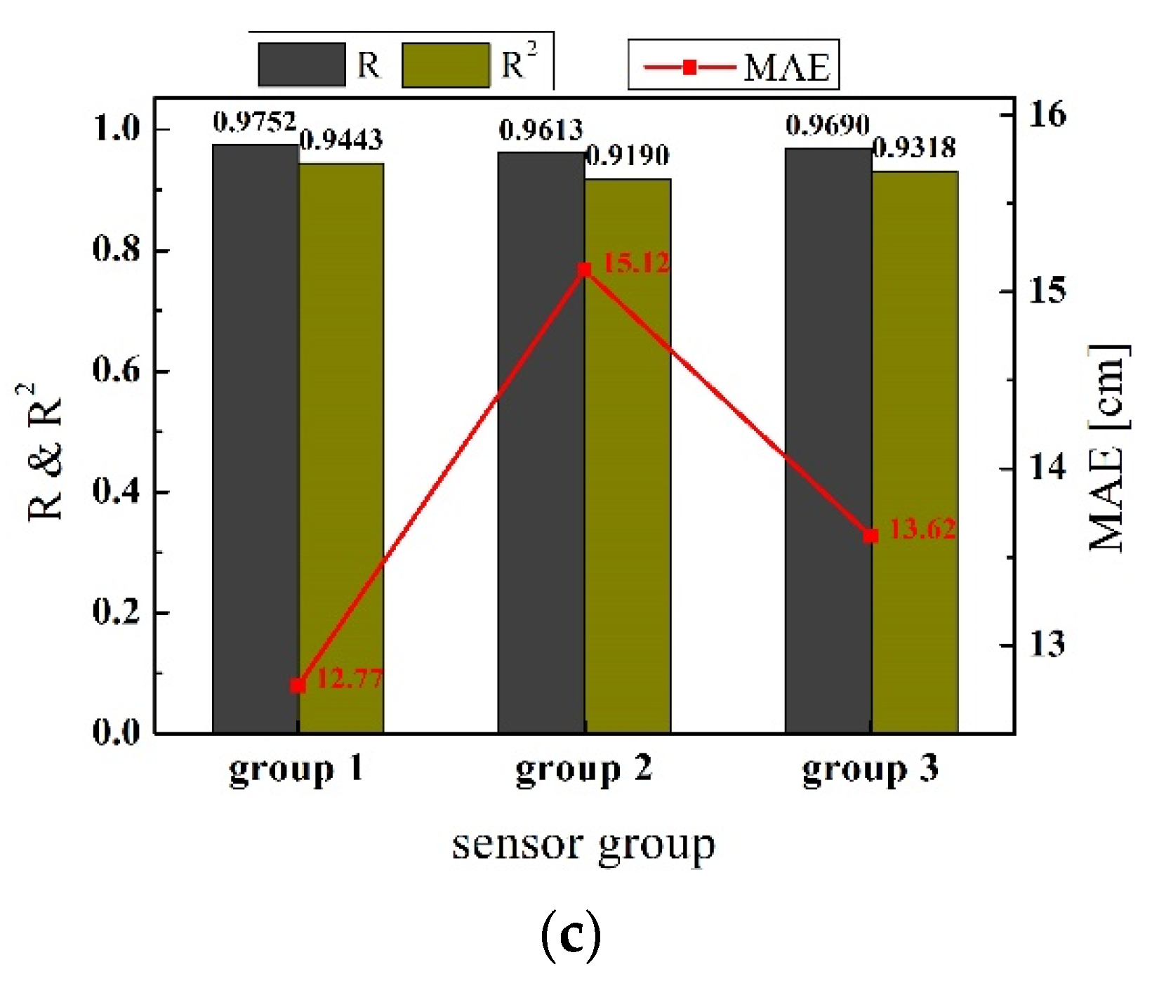
Evaluation results of the prediction accuracy of the three groups using scale-dependent metrics are illustrated in Table 5 and Figure 8. The values of R and R2 of the three groups were higher than 0.90, indicating that the correlations of the three regression models were very strong. However, the difference in correlations between the three groups were very small.
The evaluation results of MSE, RMSE and MAE for group 3 were 315.45 cm2, 17.76 cm and 13.62 cm, respectively. The group 3 was a reference for group 1 and group 2, because dataset 3 (dataset of group 3) was a combination of dataset 1 and dataset 2. The evaluation results of MSE, RMSE and MAE for group 1 were 249.02 cm2, 15.78 cm and 12.77 cm, and the evaluation results of group 1 were smaller than the evaluation results of group 3. The evaluation results of MSE, RMSE, and MAE for group 2 were 402.15 cm2, 20.05 cm and 15.12 cm, and the evaluation results of group 2 were greater than the evaluation results of group 3. According to the evaluation results, the prediction errors of the three groups can be ranked as follows: group 2 > group 3 > group 1.

4.2.2. Evaluations of Prediction Accuracy Using Percentage-Dependent Metrics

Table 6 and Figure 9 illustrate the evaluation results of the prediction accuracy of the three groups using percentage-dependent metrics. Due to the existence of zero values in the actual values, the evaluation results of the MAPE were infinite. After removing the zero values from actual values, the value of the MAPE was calculated accurately. The evaluation results of the MAPE of group 1, group 2 and group 3 were, 14.27%, 17.16% and 14.61%, respectively.
The existences of zero values in actual values affected the calculation accuracy of the SMAPE as shown in Table 6. When including the zero values in the actual values, the calculation results of the SMAPE of group 1, group 2 and group 3 were 52.02%, 56.17% and 52.94%. After removing the zero values from the actual values, the calculation results of the SMAPE decreased to 15.07%, 18.05% and 15.17%, respectively.
The evaluation results of the three groups using scale-dependent metrics and percentage-dependent metrics showed that the prediction accuracy of group 1 was the best, group 3 was second and group 2 was third. In other words, the training dataset based on the 300 AE signals collected from the pile-installed sensors (S1, S2 and S3) showed better performance for training the ANN prediction model than the training dataset based on the 300 AE signals collected from the platform-installed sensors (S4, S5, and S6). The accuracy of the training dataset based on the 600 AE signals collected from the mix-installed sensors (S1, S2, S3, S4, S5, and S6) was between those two groups.
From the evaluation results, engineers can consider that, when detecting pile foundations, it should be the first option to install AE sensors on the pile body to receive AE signals to detect damage locations. The method of mix-installation can be the second option, and the method of platform-installation should be the last option.

5. Discussion

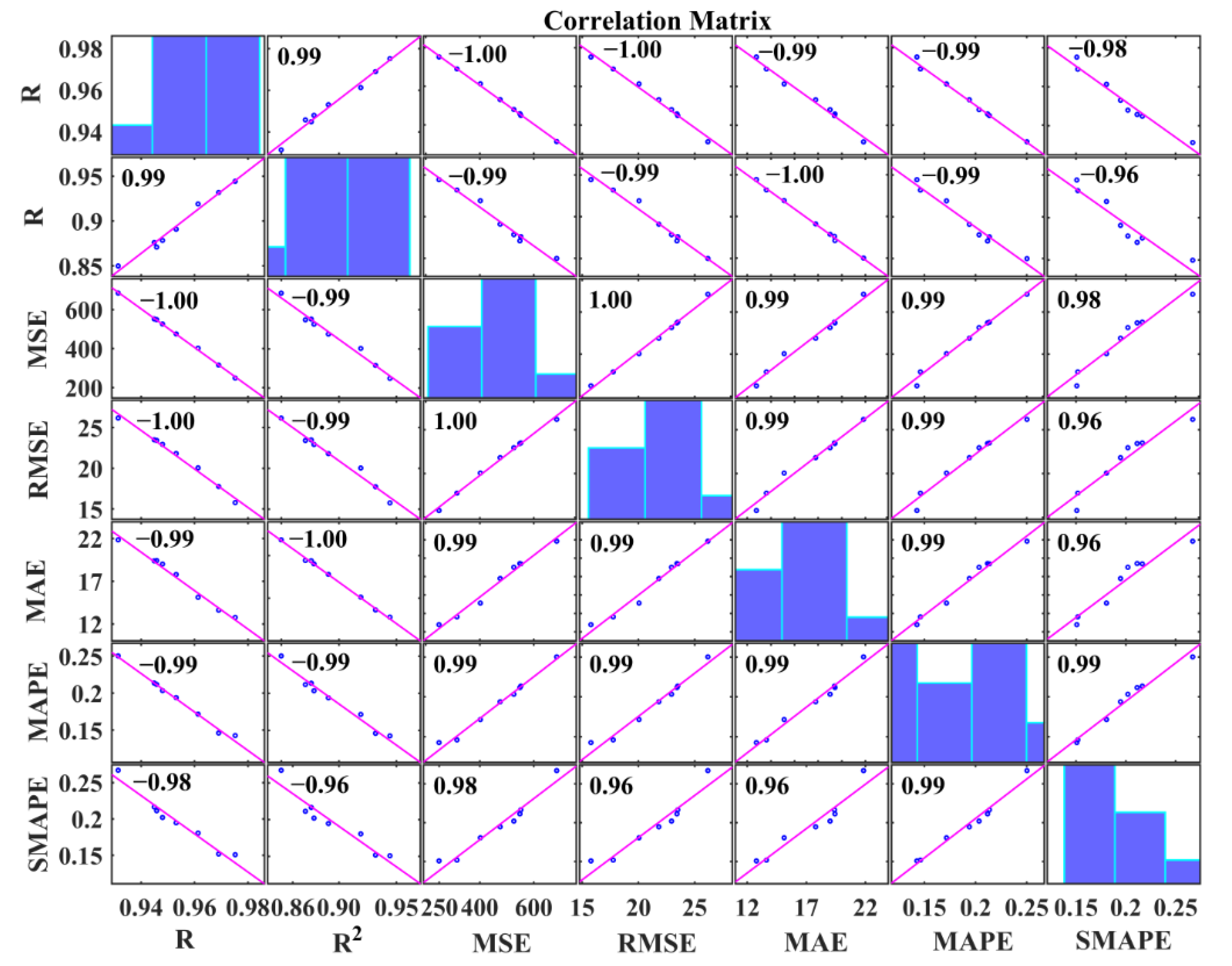
It is not necessary to use all metrics when evaluating the accuracy of a prediction result. As a matter of fact, one or two accuracy metrics are sufficient for evaluation. To determine the best option, clarifying the correlations between different accuracy metrics is an important issue. Figure 10 shows the correlation matrix of the seven accuracy metrics. In the correlation matrix, the Pearson correlation coefficient values were calculated using all evaluation results of the accuracy metrics (refer to Table 3, Table 4, Table 5 and Table 6).
As can be seen from the correlation matrix, the correlation coefficients of any two metrics were greater than 0.95. This indicates that the accuracy metrics have strong correlations with each other. In detail, the correlation coefficient of R and R2 was 0.99, the correlation coefficient of the MSE and RMSE was 1, the correlation coefficient of the MSE and MAE was 0.99, and the correlation coefficient of the MAPE and SMAPE was 0.99.
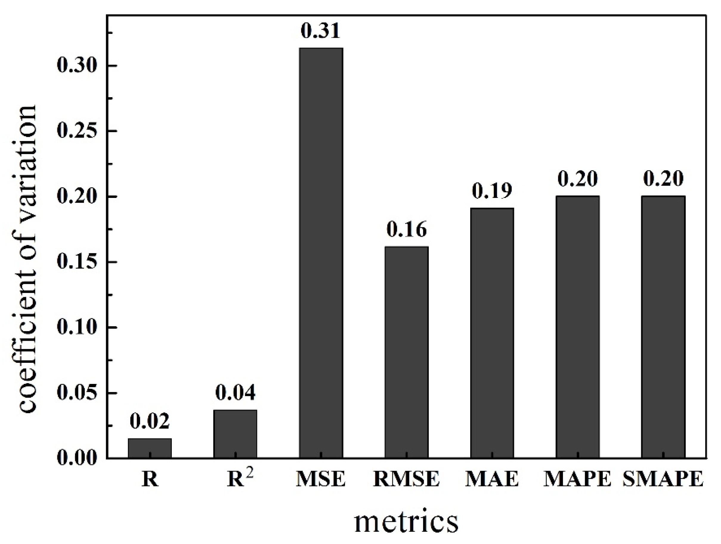
Comparing the sensitivity of metrics is helpful to determine a suitable accuracy metric. In this study, the sensitivity of accuracy metrics was defined using the coefficient of variation (CV). The CV is a statistical measure of the dispersion of data points around the mean value. Higher CV values highlight results more sensitive to the predictions. The CV is illustrated by Equation (11):
CV = s u
where s is the standard deviation and u is the mean value.
According to the evaluation results of each metric (refer to Table 3, Table 4, Table 5 and Table 6), the CV of each metric was calculated as shown in Figure 11. The CV values of R, R2, MSE, RMSE, MAE, MAPE and SMAPE were 0.02, 0.04, 0.31, 0.16, 0.19, 0.20 and 0.20, respectively.
For correlation-based metrics, R2 is more sensitive to the prediction results. For scale-dependent metrics, the MSE is more sensitive than RMSE and MAE. That is why the MSE is the default evaluation metric in many machine learning algorithms. For percentage-dependent metrics, the sensitivities of the MAPE and SMAPE are the same.
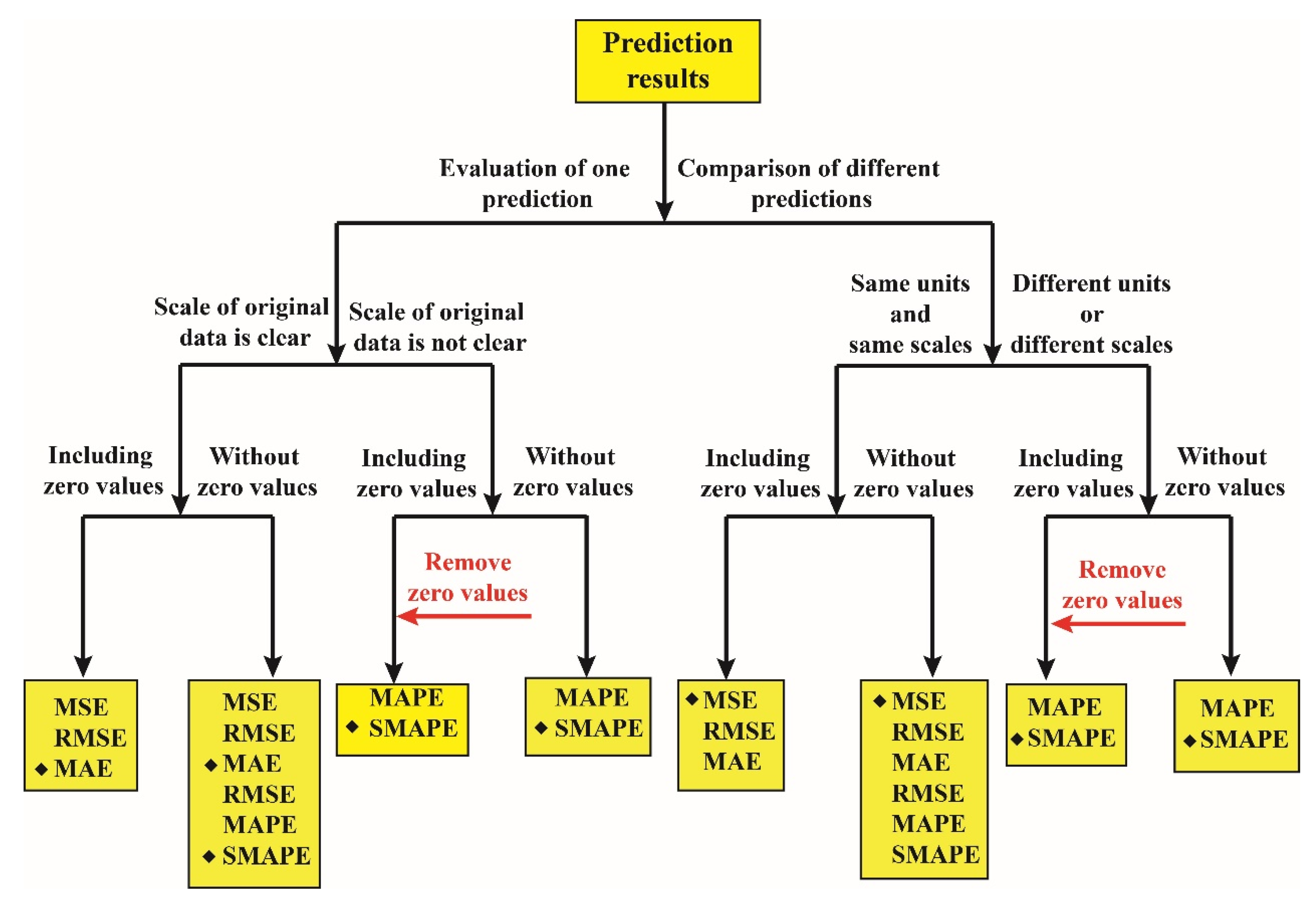
Based on the findings of this study, the proposed novel selection method of an appropriate accuracy metric for evaluating prediction results is as shown in Figure 12. First of all, it should be clarified that the purpose of this work was to evaluate the accuracy of a prediction or to compare the accuracy of different predictions.
To evaluate the accuracy of a prediction result, it is necessary to clarify whether the scale of original data is clear or not. When the scale of original data is clear, both scale-dependent metrics and percentage-dependent metrics are options under the circumstances of results being without zero values in the actual values. Of these, the MAE is recommended from the scale-dependent metrics because the unit of the MAE is the same as the original data and easy to understand. The SMAPE is recommended as the appropriate metric of the percentage-dependent metrics. In comparison with the MAPE, the SMAPE places same penalty on both positive error and negative error. When the actual values include zero values, only the scale-dependent metrics are available, and the MAE is therefore recommended.
When the scale of original data is not clear, the percentage-dependent metrics are appropriate for evaluation. If there are zero values in the actual values, the zero values should be removed from the actual values before using percentage-dependent metrics for evaluation. The SMAPE is recommended as the appropriate metric in this case.
When comparing the accuracy of different predictions, it is necessary to clarify whether the units of the original data of different predictions are the same or not, and whether the scales of the original data are the same or not. When both the units and scales of the original data are the same, the MSE is recommended as the best option for comparing the accuracy of different predictions because the MSE is more sensitive to errors than other metrics and more useful to compare different predictions.
When the units or scales of the original data are different, only the percentage-dependent metrics are available for evaluation. In this case, the SMAPE is recommended as the appropriate metric. If there are zero values in the actual values, the zero values should be removed from the actual values before using the SMAPE.

6. Conclusions

This study included experimental studies and analytical investigations to propose a new method to evaluate the prediction accuracy of damage locations using ANN with AE data in deep piles. The main conclusions drawn from the results are as follows:
  • Among the six training algorithms studied in this paper, the training algorithm of “TRAINGLM” has the best performance for training the ANN model for predicting damage locations in deep piles.
  • The prediction accuracies of three sensor installation groups can be ranked as follows: group 1 (pile body-installation group) > group 3 (mix-installation group) > group 2 (platform-installation group). This result can lead engineers to decide that when detecting the damages of deep piles using the AE technique, the priority AE sensor installation option is pile body-installation, the second option is mix-installation (pile body and platform), and the last option is platform-installation.
  • The existence of zero values in actual values makes the MAPE infinite, and zero values can maximize the evaluation results of the SMAPE. Thus, when evaluating the accuracy of predictions using the MAPE and SMAPE, the zero values should be removed from the actual values. The result is suitable for every prediction.
  • The sensitivity of the seven accuracy metrics can be ranked as follows: MSE > SMAPE = MAPE > MAE > RMSE > R2 > R. The more sensitive the metric is, the more suitable it is for comparing the accuracy of different predictions. The result is suitable for every prediction.
In further study, the study of the training algorithms will be extended further than the six algorithms studied in this paper. The study will be extended from a single pile to group pile.

Author Contributions

Conceptualization, A.J., S.W. and T.-M.O.; data curation, A.J.; formal analysis, A.J. and P.W.; Funding acquisition, S.W. and P.W.; software, A.J. and T.-M.O.; writing—original draft preparation, A.J.; writing—review and editing, S.W. and T.-M.O.; project administration, S.W. All authors have read and agreed to the published version of the manuscript.

Funding

This work was conducted with supports from the National Natural Science Foundation of China (Grant Nos. U1602232 and 51474050), Key science and technology projects of Liaoning Province, China (2019JH2-10100035), the Fundamental Research Funds for the Central Universities (N180701005).

Institutional Review Board Statement

Not applicable.

Informed Consent Statement

Not applicable.

Data Availability Statement

Data sharing is not applicable to this article.

Acknowledgments

This work was supported by the Brain Korea 21 FOUR Project in the Education & Research Center for Infrastructure of Smart Ocean City (i-SOC Center).

Conflicts of Interest

The authors declare no conflict of interest.

References

  1. Mao, W.; Aoyama, S.; Towhata, I. Feasibility study of using acoustic emission signals for investigation of pile spacing effect on group pile behavior. Appl. Acoust. 2018, 139, 189–202. [Google Scholar] [CrossRef]
  2. Mao, W.W.; Towhata, I.; Aoyama, S.; Goto, S. Grain Crushing under Pile Tip Explored by Acoustic Emission. Geotech. Eng. 2016, 47, 164–175. [Google Scholar]
  3. Vélez, W.; Matta, F.; Ziehl, P. Acoustic emission monitoring of early corrosion in prestressed concrete piles. Struct. Control Health Monit. 2015, 22, 873–887. [Google Scholar] [CrossRef]
  4. Kumar, K.V.; Saravanan, T.J.; Sreekala, R.; Gopalakrishnan, N.; Mini, K.M. Structural damage detection through longitudinal wave propagation using spectral finite element method. Geomech. Eng. 2017, 12, 161–183. [Google Scholar] [CrossRef]
  5. Mao, W.; Yang, Y.; Lin, W. An acoustic emission characterization of the failure process of shallow foundation resting on sandy soils. Ultrasonics 2019, 93, 107–111. [Google Scholar] [CrossRef] [PubMed]
  6. Wu, Y.; Li, S.; Wang, D.; Zhao, G. Damage monitoring of masonry structure under in-situ uniaxial compression test using acoustic emission parameters. Constr. Build. Mater. 2019, 215, 812–822. [Google Scholar] [CrossRef]
  7. Kim, Y.-M.; Han, G.; Kim, H.; Oh, T.-M.; Kim, J.-S.; Kwon, T.-H. An Integrated Approach to Real-Time Acoustic Emission Damage Source Localization in Piled Raft Foundations. Appl. Sci. 2020, 10, 8727. [Google Scholar] [CrossRef]
  8. Grosse, C.; Ohtsu, M. Acoustic Emission Testing: Basics for Research-Applications in Civil Engineering; Springer: Berlin/Heidelberg, Germany, 2008; pp. 1–10. [Google Scholar] [CrossRef]
  9. Wang, S.; Huang, R.; Ni, P.; Pathegama Gamage, R.; Zhang, M. Fracture Behavior of Intact Rock Using Acoustic Emission: Experimental Observation and Realistic Modeling. Geotech. Test. J. 2013, 36, 903–914. [Google Scholar] [CrossRef] [Green Version]
  10. Cortés, G.; Suarez Vargas, E.; Gallego, A.; Benavent-Climent, A. Health monitoring of reinforced concrete structures with hysteretic dampers subjected to dynamical loads by means of the acoustic emission energy. Struct. Health Monit. 2018, 18. [Google Scholar] [CrossRef]
  11. Glowacz, A. Acoustic fault analysis of three commutator motors. Mech. Syst. Signal Process. 2019, 133, 106226. [Google Scholar] [CrossRef]
  12. Arakawa, K.; Matsuo, T. Acoustic Emission Pattern Recognition Method Utilizing Elastic Wave Simulation. Mater. Trans. 2017, 58, 1411–1417. [Google Scholar] [CrossRef]
  13. Gelman, L.; Kırlangıç, A.S. Novel vibration structural health monitoring technology for deep foundation piles by non-stationary higher order frequency response function. Struct. Control Health Monit. 2020, 27, e2526. [Google Scholar] [CrossRef]
  14. Zhou, G.; Ji, Y.C.; Chen, X.D.; Zhang, F.F. Artificial Neural Networks and the Mass Appraisal of Real Estate. Int. J. Online Eng. 2018, 14, 180–187. [Google Scholar] [CrossRef] [Green Version]
  15. Wu, Y.-c.; Feng, J.-w. Development and Application of Artificial Neural Network. Wirel. Pers. Commun. 2018, 102, 1645–1656. [Google Scholar] [CrossRef]
  16. Anitescu, C.; Atroshchenko, E.; Alajlan, N.; Rabczuk, T. Artificial Neural Network Methods for the Solution of Second Order Boundary Value Problems. Comput. Mater. Contin. 2019, 59, 345–359. [Google Scholar] [CrossRef] [Green Version]
  17. Benzer, R. Population dynamics forecasting using artificial neural networks. Fresenius Environ. Bull. 2015, 12, 14–26. [Google Scholar]
  18. Al-Jumaili, S.K.; Pearson, M.R.; Holford, K.M.; Eaton, M.J.; Pullin, R. Acoustic emission source location in complex structures using full automatic delta T mapping technique. Mech. Syst. Signal Process. 2016, 72–73, 513–524. [Google Scholar] [CrossRef]
  19. Ebrahimkhanlou, A.; Dubuc, B.; Salamone, S. A generalizable deep learning framework for localizing and characterizing acoustic emission sources in riveted metallic panels. Mech. Syst. Signal Process. 2019, 130, 248–272. [Google Scholar] [CrossRef]
  20. Ebrahimkhanlou, A.; Salamone, S. Single-Sensor Acoustic Emission Source Localization in Plate-Like Structures Using Deep Learning. Aerospace 2018, 5, 50. [Google Scholar] [CrossRef] [Green Version]
  21. Hussain, D.; Khan, A.A. Machine learning techniques for monthly river flow forecasting of Hunza River, Pakistan. Earth Sci. Inform. 2020, 13, 939–949. [Google Scholar] [CrossRef]
  22. Alghamdi, A.S.; Polat, K.; Alghoson, A.; Alshdadi, A.A.; Abd El-Latif, A.A. Gaussian process regression (GPR) based non-invasive continuous blood pressure prediction method from cuff oscillometric signals. Appl. Acoust. 2020, 164. [Google Scholar] [CrossRef]
  23. Alghamdi, A.S.; Polat, K.; Alghoson, A.; Alshdadi, A.A.; Abd El-Latif, A.A. A novel blood pressure estimation method based on the classification of oscillometric waveforms using machine-learning methods. Appl. Acoust. 2020, 164. [Google Scholar] [CrossRef]
  24. Nandy, A. Statistical methods for analysis of Parkinson’s disease gait pattern and classification. Multimed. Tools Appl. 2019, 78, 19697–19734. [Google Scholar] [CrossRef]
  25. Naz, A.; Javed, M.U.; Javaid, N.; Saba, T.; Alhussein, M.; Aurangzeb, K. Short-Term Electric Load and Price Forecasting Using Enhanced Extreme Learning Machine Optimization in Smart Grids. Energies 2019, 12, 866. [Google Scholar] [CrossRef] [Green Version]
  26. Qiu, G.Q.; Gu, Y.K.; Chen, J.J. Selective health indicator for bearings ensemble remaining useful life prediction with genetic algorithm and Weibull proportional hazards model. Measurement 2020, 150. [Google Scholar] [CrossRef]
  27. Popoola, S.I.; Jefia, A.; Atayero, A.A.; Kingsley, O.; Faruk, N.; Oseni, O.F.; Abolade, R. Determination of Neural Network Parameters for Path Loss Prediction in Very High Frequency Wireless Channel. IEEE Access 2019, 7, 150462–150483. [Google Scholar] [CrossRef]
  28. Kvålseth, T.O. Cautionary Note about R 2. Am. Stat. 1985, 39, 279–285. [Google Scholar] [CrossRef]
  29. Wang, W.C.; Chau, K.W.; Cheng, C.T.; Qiu, L. A comparison of performance of several artificial intelligence methods for forecasting monthly discharge time series. J. Hydrol. 2009, 374, 294–306. [Google Scholar] [CrossRef] [Green Version]
  30. Jamei, M.; Ahmadianfar, I.; Chu, X.F.; Yaseen, Z.M. Prediction of surface water total dissolved solids using hybridized wavelet-multigene genetic programming: New approach. J. Hydrol. 2020, 589. [Google Scholar] [CrossRef]
  31. Ali, M.; Prasad, R.; Xiang, Y.; Deo, R.C. Near real-time significant wave height forecasting with hybridized multiple linear regression algorithms. Renew. Sustain. Energy Rev. 2020, 132, 110003. [Google Scholar] [CrossRef]
  32. Bucchianico, A.D. Coefficient of Determination (R2). In Encyclopedia of Statistics in Quality and Reliability; John Wiley & Sons, Ltd: New Jersey, NY, USA, 2008. [Google Scholar] [CrossRef]
  33. Kim, S.; Alizamir, M.; Zounemat-Kermani, M.; Kisi, O.; Singh, V.P. Assessing the biochemical oxygen demand using neural networks and ensemble tree approaches in South Korea. J. Environ. Manag. 2020, 270. [Google Scholar] [CrossRef] [PubMed]
  34. Hyndman, R.J. Another Look at Forecast Accuracy Metrics for Intermittent Demand. Foresight Int. J. Appl. Forecast. 2006, 4, 43–46. [Google Scholar]
  35. Sanders, N.R. Measuring forecast accuracy: Some practical suggestions. Prod. Inventory Manag. J. 1997, 38, 43–46. [Google Scholar]
  36. Flores, B.E. A pragmatic view of accuracy measurement in forecasting. Omega 1986, 14, 93–98. [Google Scholar] [CrossRef]
  37. Kim, C.H.; Kim, Y.C. Application of Artificial Neural Network Over Nickel-Based Catalyst for Combined Steam-Carbon Dioxide of Methane Reforming (CSDRM). J. Nanoence Nanotechnol. 2020, 20, 5716–5719. [Google Scholar] [CrossRef] [PubMed]
  38. Rakićević, Z.; Vujosevic, M. Focus forecasting in supply chain: The Case study of fast moving consumer goods company in Serbia. Serb. J. Manag. 2014, 10. [Google Scholar] [CrossRef] [Green Version]
  39. Armstrong, J.S.; Collopy, F. Error measures for generalizing about forecasting methods: Empirical comparisons. Int. J. Forecast. 1992, 8, 69–80. [Google Scholar] [CrossRef] [Green Version]
  40. Khac Le, H.; Kim, S. Machine Learning Based Energy-Efficient Design Approach for Interconnects in Circuits and Systems. Appl. Sci. 2021, 11, 915. [Google Scholar] [CrossRef]
  41. Wu, P.; Che, A. Spatiotemporal Monitoring and Evaluation Method for Sand-Filling of Immersed Tube Tunnel Foundation. Appl. Sci. 2021, 11, 1084. [Google Scholar] [CrossRef]
  42. Zhu, C.; Zhang, J.; Liu, Y.; Ma, D.; Li, M.; Xiang, B. Comparison of GA-BP and PSO-BP neural network models with initial BP model for rainfall-induced landslides risk assessment in regional scale: A case study in Sichuan, China. Nat. Hazards J. Int. Soc. Prev. Mitig. Nat. Hazards 2020, 100, 173–204. [Google Scholar] [CrossRef]
  43. Silitonga, P.; Bustamam, A.; Muradi, H.; Mangunwardoyo, W.; Dewi, B.E. Comparison of Dengue Predictive Models Developed Using Artificial Neural Network and Discriminant Analysis with Small Dataset. Appl. Sci. 2021, 11, 943. [Google Scholar] [CrossRef]
  44. Pimentel-Mendoza, A.B.; Rico-Pérez, L.; Rosel-Solis, M.J.; Villarreal-Gómez, L.J.; Vega, Y.; Dávalos-Ramírez, J.O. Application of Inverse Neural Networks for Optimal Pretension of Absorbable Mini Plate and Screw System. Appl. Sci. 2021, 11, 1350. [Google Scholar] [CrossRef]
  45. Pandey, S.; Hindoliya, D.A.; Mod, R. Artificial neural networks for predicting indoor temperature using roof passive cooling techniques in buildings in different climatic conditions. Appl. Soft Comput. 2012, 12, 1214–1226. [Google Scholar] [CrossRef]
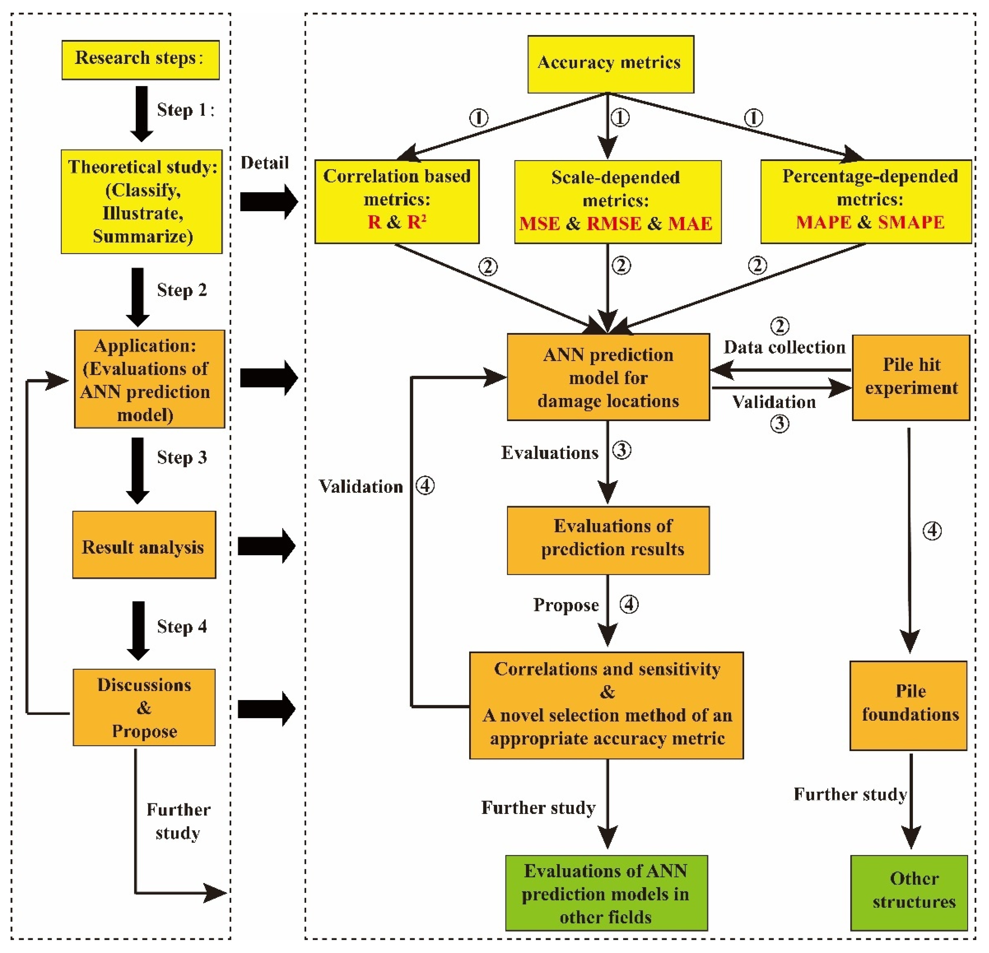
Figure 1. Step-by-step block diagram of the proposed research. Step 1: theoretical study; step 2: application of accuracy metrics; step 3: result analysis; step 4: discussion and proposal of a novel selection method. ANN: artificial neural network; MSE: mean square error; RMSE: root mean square error; MAE: mean absolute error; MAPE: mean absolute percentage error; SMAPE: symmetric mean absolute percentage error.
Applsci 11 02314 g001
Figure 2. Degree of correlations. Five degrees of correlations: very weak (from 0.0 to 0.2 or from 0.0 to −0.2), weak (from 0.2 to 0.4 or from −0.2 to −0.4), moderate (from 0.4 to 0.6 or from −0.4 to −0.6), strong (from 0.6 to 0.8 or from −0.6 to −0.8), very strong (from 0.8 to 1.0 or from −1.8 to −1.0).
Applsci 11 02314 g002
Figure 3. Experimental setup of the pile hit test. (a) Two-dimensional sketch of experimental setup. (b) Three-dimensional sketch of experimental setup. (c) Cross-section of the pile. (d) Hit process. (e) Hammer. (f) Input signal. (g) AE data acquisition system (Micro-II Digital AE system). (h) R.45IC-type AE sensor.
Applsci 11 02314 g003
Figure 4. Schematic diagram of backpropagation ANN prediction model for damage locations. In the ANN prediction model, AE signals were input from the input layer and the damage locations output from the output layer. There were 10 neurons in the hidden layer.
Applsci 11 02314 g004
Figure 5. Regression plot of the six training algorithms. (a) Regression plot of TRAINBFG; R value is 0.9449. (b) Regression plot of TRAINCGB; R value is 0.9480. (c) Regression plot of TRAINCGP; R value is 0.9314. (d) Regression plot of TRAINGLM; R value is 0.9690. (e) Regression plot of TRAINRP; R value is 0.9531. (f) Regression plot of TRAINSCG; R value is 0.9458.
Applsci 11 02314 g005
Figure 6. Evaluation results of six training algorithms using scale-dependent metrics. (a) Evaluation results using MSE. (b) Evaluation results using RMSE. (c) Evaluation results using MAE. The evaluation results of “TRAINGLM” are minimum, and the evaluation results of “TRAINCGP” are maximum. Abbreviations: (1) BFG: TRAINBFG, (2) CGB: TRAINCGB, (3) CGP: TRAINCGP, (4) GLM: TRAINGLM, (5) RP: TRAINRP, (6) SSG: TRAINSCG.
Applsci 11 02314 g006
Figure 7. Evaluation results of six training algorithms using percentage-dependent metrics. Evaluation results of the “TRAINGLM” are minimum, and evaluation results of the “TRAINCGP” are maximum.
Applsci 11 02314 g007
Figure 8. Evaluation results of different group datasets using scale-dependent metrics. (a) Evaluation results using MSE. (b) Evaluation results using RMSE. (c) Evaluation results using MAE. The evaluation results of group 1 are minimum, and the evaluation results of group 2 are maximum.
Applsci 11 02314 g008aApplsci 11 02314 g008b
Figure 9. Evaluation results of different group datasets using percentage-dependent metrics. The evaluation results of group 1 are minimum, and the evaluation results of group 2 are maximum.
Applsci 11 02314 g009
Figure 10. Correlation matrix of accuracy metrics. The purple line is the correlation line between two metrics, the number is the Pearson correlation coefficient value (refer to Figure 2).
Applsci 11 02314 g010
Figure 11. Coefficient of variations of each metric.
Applsci 11 02314 g011
Figure 12. Schematic diagram of the novel selection method for accuracy metrics (the “◆” refers to the recommended metric for this case).
Applsci 11 02314 g012
Table 1. Operating specifications of R.45IC type AE sensor.
Operating SpecificationsValue
DynamicPeak Sensitivity, Ref V(m/s)124 dB
Operating Frequency Range1–30 kHz
Resonant Frequency, Ref V(m/s)20 kHz
EnvironmentalTemperature Range−35 °C–−75 °C
Shock Limit500 g
PhysicalDimensions28.6 mm OD × 50 mm H
Weight121 g
ElectricalGain40 dB
Power requirements20–30 VDC @ 25 mA
Dynamic Range>87 dB
Table 2. The illustrations of abbreviation and functions of the six training algorithms.
AlgorithmDescription
TRAINBFGIt is a network training algorithm that updates weight and bias values in terms of the BFGS quasi-Newton method.
TRAINCGBIt is a network training algorithm that updates weight and bias values in terms of the conjugate gradient backpropagation with Powell-Beale restarts.
TRAINCGPIt is a network training algorithm that updates weight and bias values in terms of conjugate gradient backpropagation with Polak-Ribiére updates.
TRAINGLMIt is a network training algorithm that updates weight and bias values in terms of Levenberg-Marquardt optimization.
TRAINRPIt is a network training algorithm that updates weight and bias values in terms of the resilient backpropagation algorithm (Rprop).
TRAINSCGIt is a network training algorithm that updates weight and bias values in terms of the scaled conjugate gradient method.
Table 3. Evaluation results of six training algorithms using scale-dependent metrics.
AlgorithmRR2MSE (cm2)RMSE (cm)MAE (cm)
TRAINBFG0.94490.8760552.0323.4919.38
TRAINCGB0.9480 0.8784526.1922.9419.01
TRAINCGP0.93140.8499685.0326.1721.84
TRAINGLM0.96900.9318315.4517.7613.62
TRAINRP0.9531 0.8909475.5021.8117.79
TRAINSCG0.94580.8709548.5923.4219.42
Table 4. Evaluation results of six training algorithms using percentage-dependent metrics.
GroupRR2MPAE
(Include Zero Values)
MAPE
(Remove Zero Values)
SMAPE
(Include Zero Values)
SMAPE
(Remove Zero Values)
TRAINBFG0.94490.8760Infinite21.35 %58.09 %21.65 %
TRAINCGB0.94800.8784Infinite20.34 %56.94 %20.20 %
TRAINCGP0.93140.8499Infinite25.02 %62.12 %26.71 %
TRAINGLM0.96900.9318Infinite14.61 %52.94 %15.17 %
TRAINRP0.95310.8909Infinite19.39 %56.35 %19.46 %
TRAINSCG0.94580.8709Infinite21.17 %57.68 %21.13 %
Table 5. Evaluation results of different group datasets using scale-dependent metrics.
GroupRR2MSE (cm2)RMSE (cm)MAE (cm)
Group 10.97520.9443249.0215.7812.77
Group 20.96130.9190402.1520.0515.12
Group 30.96900.9318315.4517.7613.62
Table 6. Evaluation results of different training datasets using percentage-dependent metrics.
GroupRR2MAPE
(Including Zero Values)
MAPE
(Remove Zero Values)
SMAPE
(Including Zero Values)
SMAPE
(Remove Zero Values)
Group 10.97520.9443Infinite14.27%52.02%15.07%
Group 20.96130.9190Infinite17.16%56.17%18.05%
Group 30.96900.9318Infinite14.61%52.94%15.17%
Publisher’s Note: MDPI stays neutral with regard to jurisdictional claims in published maps and institutional affiliations.