Article

Debris Flow Characteristics in Flume Experiments Considering Berm Installation

School of Civil Engineering, Chungbuk National University, Cheongju 28644, Korea
*
Author to whom correspondence should be addressed.
Appl. Sci. 2021, 11(5), 2336; https://doi.org/10.3390/app11052336
Submission received: 2 February 2021 / Revised: 26 February 2021 / Accepted: 2 March 2021 / Published: 6 March 2021
(This article belongs to the Special Issue Geohazards: Risk Assessment, Mitigation and Prevention)

Abstract

:
This study was conducted to identify the characteristics and mobility of debris flows and analyze the performance of a berm as a debris flow mitigation measure. The debris flow velocity, flow depth, Froude number, flow resistance coefficients, and mobility ratio were accordingly determined using the results of flume tests. To analyze the influence of the berm, the results for a straight channel test without a berm were compared with those for a single-berm channel test. The debris flow velocity was observed to increase with increasing channel slope and decreasing volumetric concentration of sediment, whereas the mobility ratio was observed to increase with increasing channel slope and volumetric concentration of sediment. In addition, it was confirmed that the installation of a berm significantly decreased the debris flow velocity and mobility ratio. This indicates that a berm is an effective method for reducing damage to areas downstream of a debris flow by decreasing its potential mobility. By identifying the effects of berms on debris flow characteristics according to the channel slope and volumetric concentration of sediment, this study supports the development of berms to serve as debris flow damage mitigation measures.

1. Introduction

The frequency of torrential rainfall has increased worldwide due to climate change caused by global warming, in turn increasing the occurrence of forest soil sediment disasters, such as landslides and debris flows [1]. Indeed, in South Korea, the occurrence of forest soil sediment disasters has increased due to the increasing frequency of torrential rainfall. The average annual area affected by the occurrence of forest soil sediment disasters in Korea was 290 ha for the period from 1980 to 1999, but significantly increased to 469 ha for the period from 2000 to 2019. In particular, a large-scale debris flow occurred in July 2011 at Mt. Woomyeon, located in an urban area, causing serious human casualties and property damage. This incident increased public interest in debris flow safety and expanded debris flow policy-making from mountainous areas to include urban areas as well [2]. It is known that debris flows can be initiated by various factors such as rainfall, snowmelt, typhoons, volcanoes, and earthquakes [3], but rainfall has been identified as the main cause of the debris flows that have occurred in Korea [4,5].
Debris flow, a type of mass movement, is a mixture composed of water and sediments of various particle sizes from clay to boulders. It is a dynamic phenomenon that moves downhill under the influence of gravity and may cause human casualties and property damage along the way [3,6,7,8,9]. Field monitoring of debris flows is difficult because they occur irregularly and exist for only a short duration of time [7,10,11]. Furthermore, it is difficult to accurately predict and respond to debris flows because they increase in scale by absorbing the sediment and water along their movement paths through strong erosive force [7,11,12,13]. Notably, the debris flow is distinguished from other mass movements because it is a sediment–water mixture, and thus can transfer momentum under the influence of grain friction, grain collision, and viscous fluid dynamics [14]. In addition, momentum transfer caused by collisions between grains in a debris flow leads to excess pore water pressure, which reduces the shear resistance of the debris flow and results in very high mobility [14]. Thus, a debris flow can produce a peak discharge dozens of times higher than that of a flood in the same watershed [15,16], and its flow characteristics may vary depending on the relative contents of water and sediment as well as the size and type of particles [3]. Therefore, it is necessary to identify the flow and deposition characteristics of debris flows and establish mitigation measures to predict and reduce the damage they cause.
Debris flow mitigation measures can be mainly divided into structural and non-structural measures. Structural mitigation measures directly reduce debris flow damage using structures installed in the path of a debris flow; erosion control dams, flexible debris flow barriers, and berms can all be considered appropriate structures for this purpose. Non-structural mitigation measures indirectly limit debris flow damage using methods such as debris flow forecasting and warning systems or land use regulations. Figure 1 shows examples of real world slopes with multiple berms. This study evaluated the use of a berm, a structural debris flow mitigation measure consisting of a small step installed on a slope that effectively disperses rainwater, reduces the momentum of debris flows, and reduces the riverbed erosion. Berms can be easily constructed at a low cost compared to other debris flow mitigation measures. Therefore, several studies applying berms as a debris flow mitigation measure have been recently conducted. VanDine [17] introduced a method of applying berms to lateral, deflection, and terminal walls serving as open debris flow control structures, and suggested major considerations for structural design. Prochaska et al. [18] pointed out that existing analysis methods for debris basins and deflection berms were not sufficient for the prediction of debris flow volume or the subsequent design of the berm geometry, impact load, and outlet, and accordingly suggested solutions and guidelines. Kim and Lee [19] performed numerical simulations by applying the finite difference method based on the mass conservation and momentum conservation equations to evaluate the behavior and mechanism of debris flow in response to the installation of berms on a slope. Sharma et al. [20] calculated the axial force, horizontal displacement, and safety factor using the finite element method to identify the stability of a slope according to the soil cohesion, the angle of internal friction, and the width and height of the berm installed upon it.
To effectively design debris flow mitigation measures, it is necessary to first calculate the main debris flow parameters, such as the potential debris volume, impact force, flow velocity, peak discharge, mobility ratio, runout distance, and total travel distance [16,21]. In particular, the flow velocity must be considered in the design of any debris flow mitigation measure because it directly influences the impact force and deposition characteristics, and is affected by the channel topography [3,15,22,23]. In the countries where studies on debris flow characteristics have been actively conducted, the debris flow process and impact force can be estimated relatively accurately [10,21,24]. Domestic studies on debris flows in South Korea, however, have been limited to trend analyses for simple experimental conditions. Numerical analysis, field observations, and flume experiments have all been previously used for research into the behavior and mechanism of debris flows. Numerical analyses provide relatively high accuracy, but it is difficult to obtain the necessary parameters through field observations, and as such, the observational data required to verify the results of such analyses are insufficient [2]. Thus, while field observations and numerical analyses are suitable for developing and testing methods to predict the behavior of debris flows, flume experiments are more suitable for conducting research on the behavior of debris flows under controlled conditions to develop related prediction equations [8]. Indeed, flume experiments are the only available method for identifying the flow and deposition characteristics of debris flows through repeatable experiments with reproducible results [25]. For these reasons, flume experiments have been mainly used in the past to identify the behaviors of debris flows.
In this study, flume experiments were therefore performed to analyze debris flow characteristics and mobility ratios according to channel slope, volumetric concentration of sediment, and presence of a berm. The flow velocity, flow depth, Froude number, and mobility ratio of the debris flows were then calculated based on the experimental observations. In addition, flow resistance coefficients were calculated by substituting the observed flow velocity and flow depth into the debris flow velocity estimation equations.

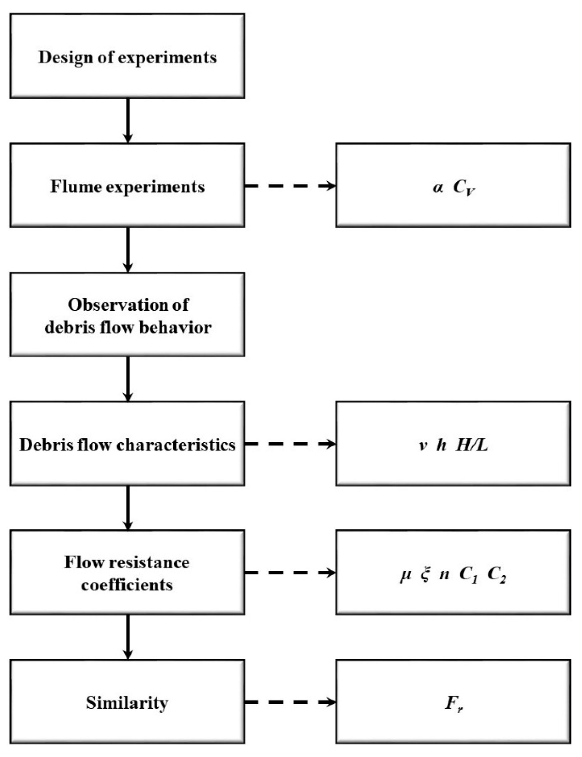
2. Methods for Assessing Debris Flow Characteristics

2.1. Flow Velocity

The debris flow velocity must be considered in any debris flow risk assessment and subsequent design of mitigation measures, because it significantly affects the impact force. It can be directly measured through field monitoring or flume experiments, or calculated using flow velocity estimation equations. The basic formula suggested in previous studies for estimating the flow velocity of a debris flow is [16,26,27,28]:
v = C h a α b
where v is the flow velocity, C is the flow resistance coefficient, h is the flow depth, α is the channel slope, and a and b are exponential factors defined according to the flow characteristics.
Table 1 defines Equations (2) through (6), which have been proposed by Hungr et al. [15], Rickenmann [16,29], Takahashi [22], Koch [26], and Lo [27]. These equations have been proposed to calculate the flow velocity for different flow types through field observations, flume experiments, and numerical analyses based on Equation (1). In Table 1, ρ is the mixed density of debris flow (kg·m−3), g is the gravitational acceleration (9.81 m·s−2), k is the cross-sectional shape factor (3 for wide rectangular channels, 5 for trapezoidal channels, and 8 for semicircular channels), μ is the apparent dynamic viscosity of the debris flow (Pa·s), ξ is the lumped coefficient depending on the volumetric concentration of sediment (m−1/2·s−1), n is the Manning coefficient (m−1/3·s), C1 is the Chezy coefficient (m1/2·s−1), and C2 is the empirical coefficient proposed by Koch [26] (m0.78·s−1). In this study, the flow resistance coefficients μ, ξ, n, C1, and C2 were calculated by substituting the experimentally observed debris flow velocity and flow depth into Equations (2) through (6).
The various coefficients in Equations (2) through (6) are empirical constants known to provide results that are reasonably consistent with field observations [27]. Hungr et al. [15] suggested that Equation (2) is suitable to estimate the debris flow velocities because a laminar flow regime is formed near the peak of debris flow surge. The variable k in Equation (2) has a different value depending on the cross-sectional shape of the channel [16]. Rickenmann [16], and Eu et al. [2], used a value of 3 as k, which is valid for a wide rectangular channel. This is because the debris flow depth is generally smaller than the width. Equation (3) is based on Bagnold’s theory [30] of dilatant grain shearing in the inertial regime. Takahashi [22] estimated the debris flow velocity based on Equation (3) and suggested that it is suitable for stony debris flows in Japan. Equation (4) is known as Manning’s formula, and Mizuyama [31] proposed using it for estimating the debris flow velocity. Equation (5) is known as Chezy’s formula, and was initially introduced to estimate the velocity of snow avalanches; Rickenmann [29] used it to estimate the debris flow velocity. Equation (6) was proposed by Koch [26] through numerical analyses. Koch [26] confirmed that the Newtonian turbulent, Voellmy, and empirical models, which have smaller exponents (a and b in Equation (1)), are closer to observed values in the field than other models.
Table 1. Equations used to estimate the mean velocity of debris flow according to flow type.
Flow TypeEquationReference
Newtonian laminar flow v = ρ g h 2 α k μ (2)[15]
Dilatant grain shearing flow v = 2 3 ξ h 3 / 2 α 1 / 2 (3)[15,22]
Newtonian turbulent flow v = 1 n h 2 / 3 α 1 / 2 (4)[15,27]
Voellmy flow v = C 1 h 1 / 2 α 1 / 2 (5)[16,26,29]
Empirical equation v = C 2 h 0.22 α 0.33 (6)[26]

2.2. Froude Number

Debris flows are dominated by the influence of gravity. Therefore, similarity must be applied using the Froude number, which represents the ratio of inertial force to gravity. The Froude number is expressed as
F r = v g h
where Fr is the Froude number.

2.3. Mobility Ratio

The debris flow mobility ratio is a dimensionless number, generally known as the Heim coefficient, obtained by dividing the total drop between the initial occurrence and final deposition points of the debris flow by the total travel distance, which is defined as the horizontal distance between the two points. This concept was introduced by Heim [32] to analyze rock avalanches, and its applicability was expanded when Iverson [14] applied it to the analysis of debris flows. The debris flow mobility ratio can be used to predict the runout distance and flow velocity [33], and many studies have used this ratio because it accurately reflects the risk and potential mobility of debris flows [8,11,14,33,34].

3. Flume Experiments

3.1. Experimental Setup

Figure 2 shows the experimental setups and main parameters of the flume experiments performed in this study. Here, H is the total drop between the initial occurrence and final deposition points of the debris flow, L is the total travel distance. The setup for the flume experiments was composed of a sample box, a channel, and a deposition plane. The sample box was 0.2 m long, 0.15 m wide, and 0.3 m high, and installed at the top of the channel. The sediment–water mixture was supplied to the channel by manually lifting the gate of the sample box. The channel was made of steel in consideration of the strong erosion that accompanies debris flow, and had a length of 1.3–1.9 m, a width of 0.15 m, and a height of 0.3 m (Table 2). The channel was fabricated in separate upper and lower slope segments so that a 0.6-m long berm could be installed between them. At the outlet of the channel, a 1.5-m long, 1.0-m wide deposition plane was installed to analyze the debris flow deposition characteristics. The deposition plane was composed of 0.05-m grids in the longitudinal and lateral directions.
To observe the flow and deposition characteristics of the debris flow, cameras capable of capturing video at 60 fps were installed at the front and on a side of the flume. The front camera was used to measure the mean velocity of the head of the debris flow from the top of the channel to the outlet, and the side camera was used to measure the maximum depth of the debris flow at a point 0.1 m upstream of the channel outlet. The debris flow mobility ratio was calculated upon the completion of sediment–water mixture deposition by observing the total drop H and total travel distance L, as indicated in Figure 2.

3.2. Experimental Conditions

Debris flows are a sediment–water mixture, thus its viscosity is difficult to measure using only a general soil test [1]. Takahashi [9] indirectly estimated the viscosity of debris flows using the volumetric concentration of sediment, and confirmed that the viscosity of debris flows increases as the volumetric concentration of sediment increases. As the viscosity of debris flows increases, the shear resistance and bed friction of the debris flows increase. This leads to a decrease in the momentum of the debris flows, which changes the debris flow characteristics. Therefore, it is necessary to compose various experimental conditions for the viscosity of debris flows. The volumetric concentration of sediment can be obtained by dividing the volume of sediment by the volume of the sediment–water mixture as follows:
C V = V S ( V S + V W ) = V S V t o t a l
where CV is the volumetric concentration of sediment, VS is the volume of sediment, VW is the volume of water, and Vtotal is the total volume of the sediment–water mixture.
In this study, the viscosity of the debris flow was also considered using CV. Table 3 shows the experimental cases evaluated in this study considering the experiment type (straight channel test or single-berm channel test), α (10–25° in 5° increments), and CV (0.40–0.60 in increments of 0.05). Consequently, a total of 40 experimental conditions were evaluated in this study, each of which was repeated five times.

3.3. Sample Properties

In this study, a sediment–water mixture was used to reproduce the conditions of a debris flow. Table 4 shows the particle composition of the sediment as determined through a sieve analysis, with reference to previous studies [35,36], and Figure 3 shows the particle-size distribution curve of the sediment. The weight ratios of each particle size range were 25% for 4.75–9.50 mm, 25% for 2.00–4.75 mm, and 50% for 2.00 mm or less. In this study, CV was set to be 0.40–0.60, based on previous studies with similar experimental setup scales [1,8,11,12]. Table 5 shows the weight of sediment and water required for each experiment when CV was adjusted within the 0.40–0.60 range, where W is the weight of the sediment-water mixture. The same volume of sediment–water mixture (4500 cm3) was used in the straight channel test and single-berm channel test. As CV increased from 0.40 to 0.60, the density of the sediment–water mixture linearly increased from 1578 to 1867 kg·m−3 (Table 5).

3.4. Experimental Method

Figure 4 and Figure 5 shows examples and a flow chart of flume experiments performed in this study, respectively. Experimental videos were separately presented in Videos S1 and S2. Flume experiments were first planned by determining the setup and conditions for each experiment, as defined in Table 3. Then, the effects of α, CV, and berm installation were examined for each of the 40 defined test conditions in the following sequence. Sediment and water were added to the sample box to meet the required weight and mixed well. The gate was then rapidly removed from the sample box to supply the sediment–water mixture. Finally, the flow velocity, flow depth, and mobility ratio of the resulting debris flow were observed as described in Section 3.1, and the flow resistance coefficient and Froude number were calculated accordingly.

4. Results and Analysis

Table 6 shows the debris flow velocity, flow depth, Froude number, total travel distance, and mobility ratio observed through the flume experiments, where N is the experiment number. In the case of the straight channel test, the development of debris flow was insufficient to observe the flow depth when α was 10° and CV was 0.60; however, debris flow was sufficiently developed when α was 15° or greater. In the single-berm channel test, debris flow stopped in the channel when CV was 0.60, regardless of α, so these values are not reported in the analysis below. In addition, when α was 20° or less and CV was between 0.50 and 0.55, the development of debris flow was insufficient to observe the flow depth in some experiments.

4.1. Debris Flow Characteristics

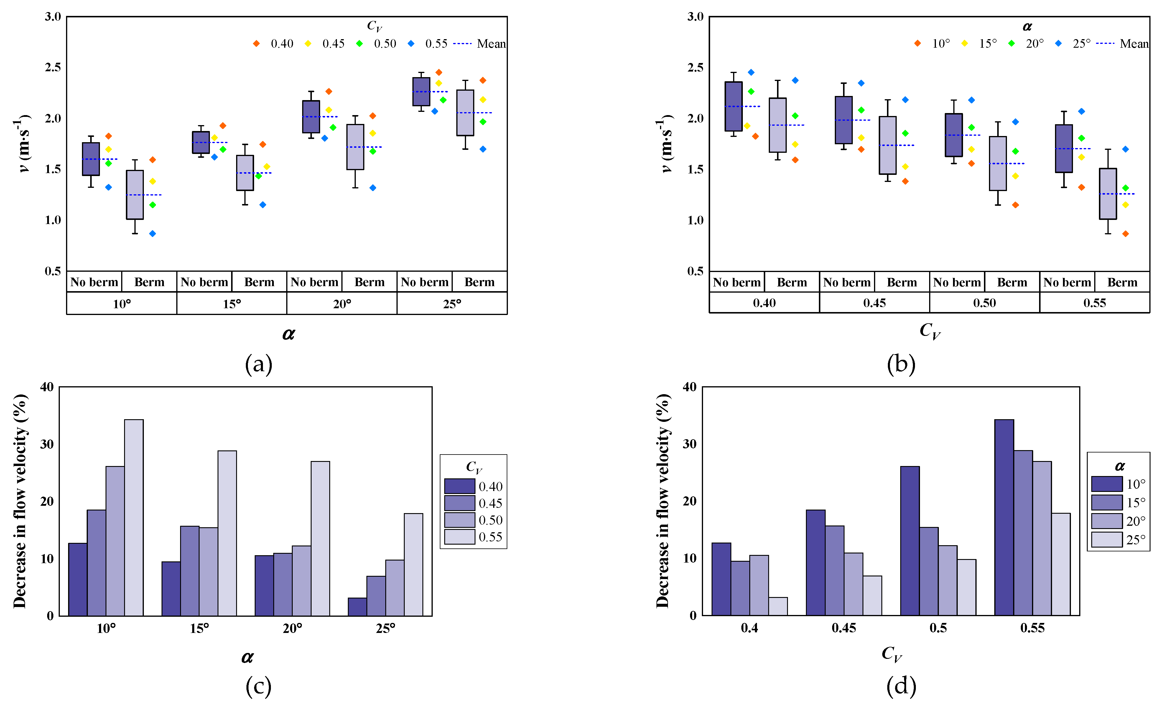
4.1.1. Flow Velocity

Figure 6 shows the flow velocities observed through the flume experiments and their changes due to the installation of the berm. Figure 6a,b show the debris flow velocity according to α and CV, respectively. Figure 6c,d show the percent change in debris flow velocity according to α and CV, respectively, after the berm was installed. The experimental results indicated that the debris flow velocity increased as α increased or CV decreased (Figure 6a,b). In the case of the straight channel test, the incremental increase in flow velocity with increasing α was similar for CV values less than 0.55, but increased noticeably with α at a higher CV. The incremental decrease in flow velocity with increasing CV was similar, regardless of α. In the case of the single-berm channel test, the incremental increase in flow velocity with increasing α was found to be similar, regardless of CV. The incremental decrease in flow velocity with increasing CV was similar when α was 15° or greater, but increased noticeably with CV when α was less than 15°. In addition, it was confirmed that the installation of the berm on the slope reduced the debris flow velocity by 3.2–34.3% (Figure 6c,d). The average decreases in debris flow velocity were found to be 22.9%, 17.4%, 15.2%, and 9.5% for a CV of 0.40–0.55 and α of 10°, 15°, 20°, and 25°, respectively, and 9.0%, 13.0%, 15.9%, and 27.0% for an α of 10°–25° and CV of 0.40, 0.45, 0.50, and 0.55, respectively. This confirmed that the installation of the berm was more effective in reducing the debris flow velocity at smaller α values and larger CV values.

4.1.2. Flow Depth

Figure 7 shows the flow depths observed through the flume experiments and their changes due to the installation of the berm. Figure 7a,b show the debris flow depth according to α and CV, respectively. Figure 7c,d show the percent change in debris flow depth according to α and CV, respectively, after the berm was installed. In the case of the straight channel test, the debris flow depth decreased as α increased or CV increased (Figure 7a,b). The decrease in flow depth with increasing α slowed when CV was 0.50 or greater, and the decrease in flow depth with increasing CV slowed when α was 15° or greater. In the case of the single-berm channel test, the debris flow depth decreased as CV increased (Figure 7b). The decrease in flow depth with increasing α changed when CV was 0.50, and the flow depth suddenly increased when α was 25° and CV was 0.45 or less (Figure 7a). The installation of the berm was found to decrease the debris flow depth by an average of 3.9–71.2%, even though the flow depth increased by 15.6% when α was 25° and CV was 0.40 (Figure 7c,d). The average decreases in debris flow depth were 43.7%, 53.8%, 44.4%, and 1.1% for a CV of 0.40–0.50 and α values of 10°, 15°, 20°, and 25°, respectively, and 25.4%, 37.6%, and 44.4% for an α of 10°–25° and CV values of 0.40, 0.45, and 0.50, respectively. This confirmed that the installation of the berm was more effective in reducing the debris flow depth at larger CV values.

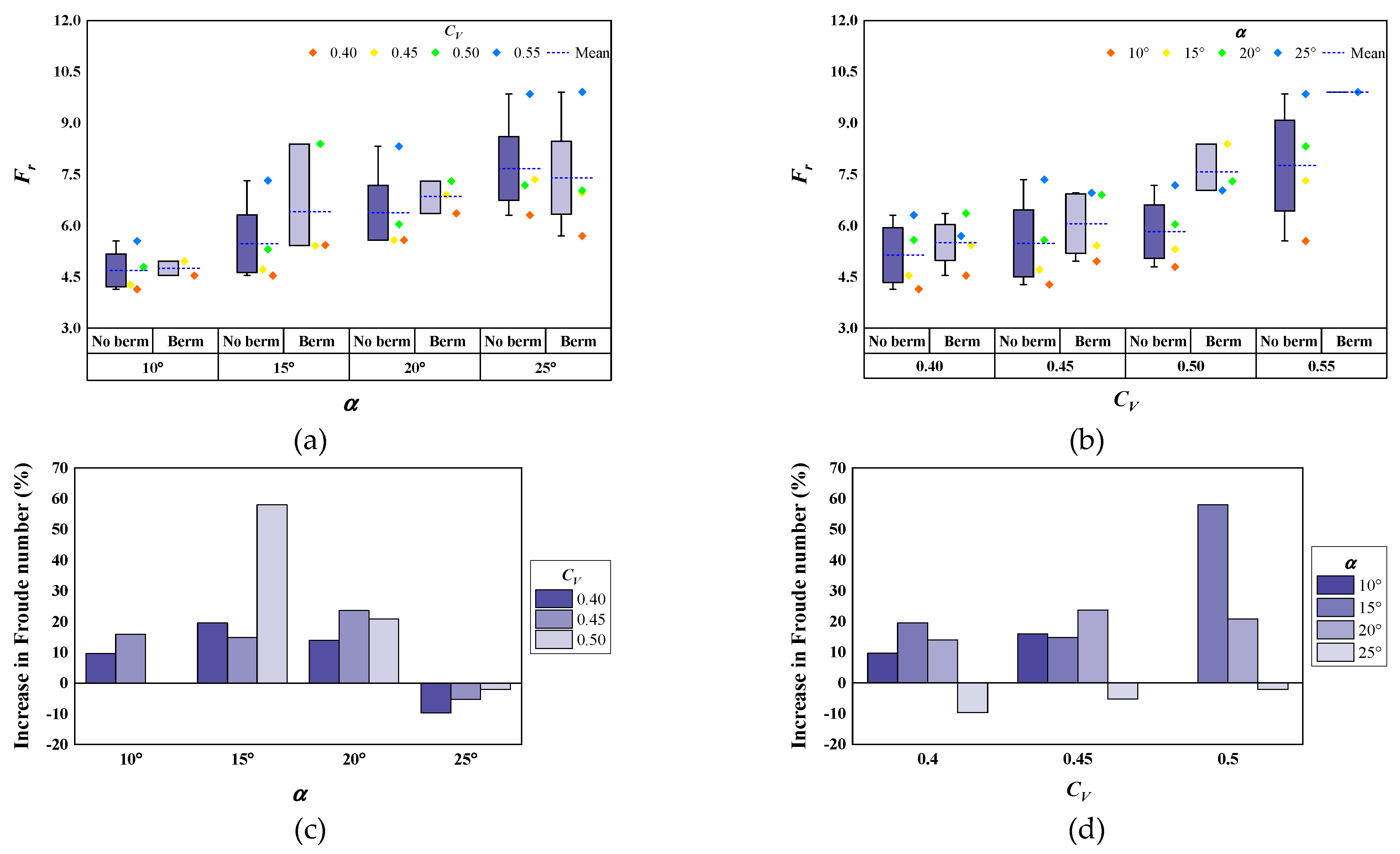
4.1.3. Froude Number

Figure 8 shows the Froude numbers calculated through the flume experiment observations and the change in Froude number due to the installation of the berm. Figure 8a,b show the Froude number according to α and CV, respectively. Figure 8c,d show the change in the Froude number according to α and CV, respectively, when the berm was installed. In the case of the straight channel test, the Froude number increased as α increased (Figure 8a). With the berm installed, the Froude number decreased by 2.1–9.7% when α was 25° and CV was 0.50 or less (Figure 8c,d); however, when α was less than 25°, the Froude number increased by 9.7–58.0% due to the installation of the berm (Figure 8c,d). The average incremental increases in the Froude number were found to be 12.8%, 30.8%, and 19.5% for a CV of 0.40–0.50 and α values of 10°, 15°, and 20°, respectively, and 8.4%, 12.3%, and 25.6% for an α of 10°–25° and CV values of 0.40, 0.45, and 0.50, respectively. In other words, the average increase in the Froude number due to the installation of the berm increased as CV increased.

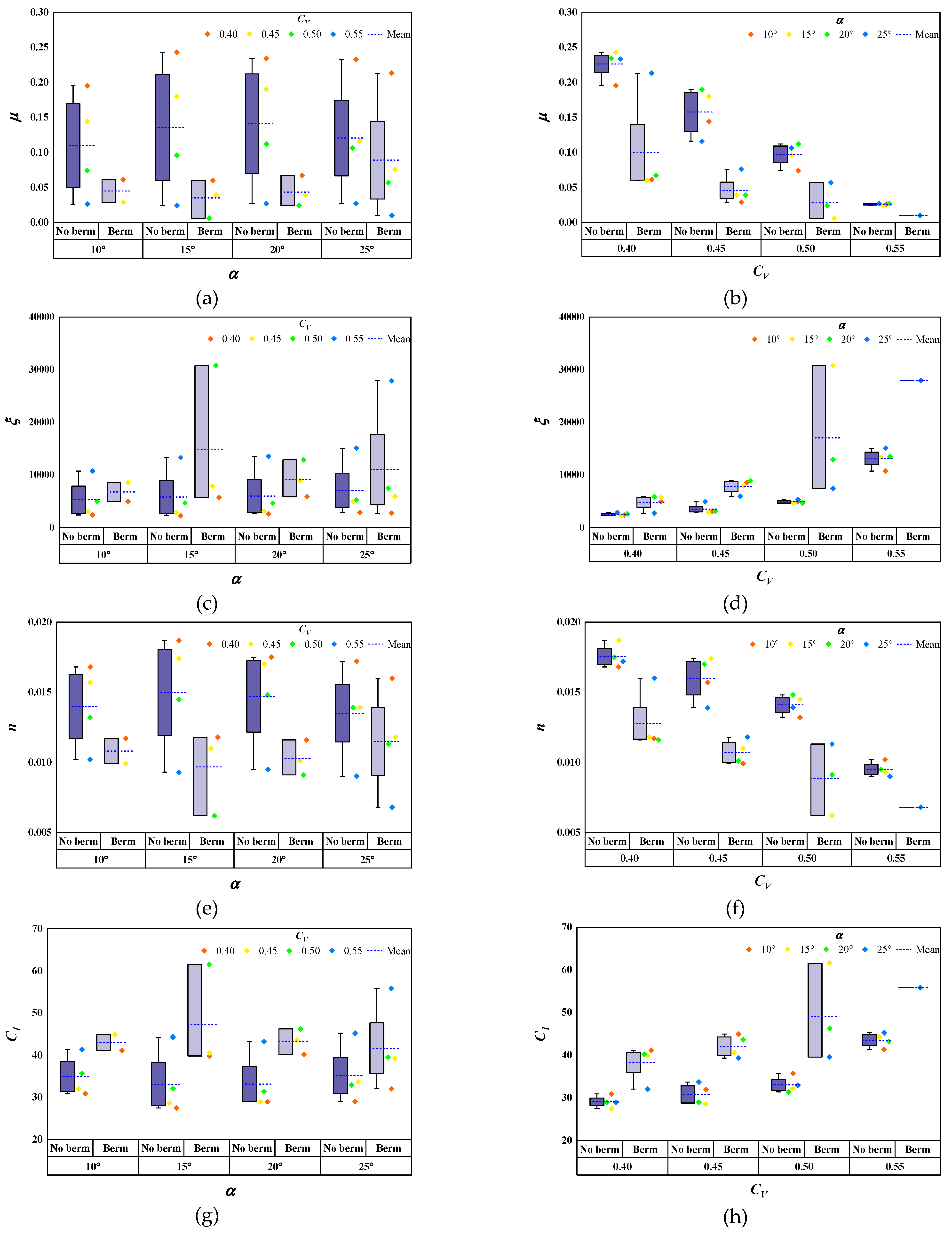
4.1.4. Flow Resistance Coefficients

Table 7 shows the ranges, mean values, and standard deviations of the flow resistance coefficients μ, ξ, n, C1, and C2 calculated using Equations (2)–(6) based on the experimental results in this study. Figure 9 shows the experimentally obtained flow resistance coefficient values according to α and CV. The experimental results showed that α had little influence on any flow resistance coefficients (Figure 9a,c,e,g,i), but CV clearly affected all flow resistance coefficients except C2 (Figure 9b,d,f,h,j): As CV increased, the values of μ and n decreased, whereas the values of ξ and C1 increased. When the berm was installed, the values of ξ decreased by 4.3% when α was 25° and CV was 0.40. Except for this one observation, each flow resistance coefficient exhibited a consistent change pattern due to the installation of the berm. The installation of the berm decreased μ by 8.6–93.8%, increased ξ by up to 563%, decreased n by 7.0–57.2%, increased C1 by 10.6–91.4%, and increased C2 by 2.9–26.4%.

4.1.5. Mobility Ratio

Figure 10 shows the debris flow mobility ratio observed through the flume experiments and the percent decrease in mobility ratio due to the installation of the berm. Figure 10a,b show the debris flow mobility ratio according to α and CV, respectively. Figure 10c,d show the percent decrease in the debris flow mobility ratio according to α and CV, respectively, when the berm was installed. The experimental results confirmed that the debris flow mobility ratio increased as α or CV increased (Figure 10a,b). In the case of the straight channel test, the incremental increases in the mobility ratio due to the increase in α were similar when CV was less than 0.55, but larger when it was 0.55 or greater. The incremental increases in mobility ratio due to the increase in CV were similar when α was 15° or greater, but considerably smaller when it was less than 15°. In the single-berm channel test, the incremental increases in the mobility ratio due to the increase in α were similar when CV was less than 0.55, but larger when it was 0.55 or higher. The incremental increases in mobility ratio due to the increase in CV were similar when α was 20° or greater, but relatively smaller when it was less than 20°. In addition, the debris flow mobility ratio was observed to decrease by 4.6–15.7% due to the installation of the berm on the slope (Figure 10c,d). The average reductions in the debris flow mobility ratio were found to be 9.8%, 9.4%, 9.1%, and 10.2% for a CV of 0.40–0.55 and α values of 10°, 15°, 20°, and 25°, respectively, and 13.6%, 10.0%, 8.2%, and 6.7% for an α of 10°–25° and CV values of 0.40, 0.45, 0.50, and 0.55, respectively. In other words, the installation of the berm was more effective in reducing the debris flow mobility ratio at lower CV values.

5. Discussion

Debris flows are affected by the characteristics of the sediment–water mixture (magnitude, CV, and grain-size distribution) and channel shape (α, width, and curvature) [3,6,9]. In this study, various α and CV values were therefore evaluated in flume tests along with changes in channel shape due to the installation of a berm in the middle of the channel. The experimental results showed that the development of a flow was influenced to occur at α of 15° (Table 6), which has been mentioned as the slope that causes debris flow in previous studies [3,9]. Takahashi [9] mentioned that the debris flow pattern suddenly changes when its CV is less than 0.55 because of active particle separation, and that a debris flow cannot reach the outlet of its channel when the CV exceeds 0.58. In this study, the development of the debris flow was also observed to differ around a CV of 0.55; at a CV of 0.60 in the single-berm channel test, the debris flow stopped in the channel before reaching the outlet (Table 6). In the straight channel test, however, it appears that α had a larger influence on the flow. Thus, debris flow occurred when α was 15° or higher, even when CV exceeded 0.58.
As α increased, the debris flow velocity and mobility ratio were both observed to increase (Figure 6a and Figure 10a). The changes in the flow velocity and mobility ratio differed around an α of 15°. The flow depth consistently decreased as α increased when no berm was installed, but it suddenly increased at an α of 25° when the berm was installed (Figure 7a). This appears to be because the debris flow moved along the steeply sloped channel with considerable momentum, and then the flow suddenly changed under the influence of the channel cross section geometry where the berm was installed. The installation of the berm caused the Froude number to increase when α was less than 25°, but it decreased when it was 25° (Figure 8c). In other words, it was confirmed that the 15° slope known to cause debris flow indeed affects the debris flow velocity and mobility ratio, and that an α of 25° affects the flow depth and Froude number in single-berm channel.
As CV increased, the debris flow velocity and flow depth decreased (Figure 6b and Figure 7b), but the mobility ratio increased (Figure 10b). A CV of 0.50 marked important the changes in the development of debris flow depth and Froude number, and a CV of 0.55 marked important changes in the development of the debris flow velocity and mobility ratio. At a CV of 0.60, the debris flow did not reach the outlet at any α when the berm was installed, but it reached the outlet if α was 15° or higher when no berm was installed. Furthermore, it was confirmed that the CV dominated the flow resistance coefficients μ, ξ, n, and C1, while C2 was not affected by the CV, likely because it was defined using a numerical analysis, unlike the other flow resistance coefficients, which were defined using the experimental results. Similarly, Rickenmann [16] mentioned that C2 is appropriate for the numerical analysis of unsteady debris flows.
The Froude numbers obtained in this study ranged from 4.14 to 10.79. This range is similar to those reported in studies conducted using an experimental setup with a channel length of 2 m or less [2,35]. The Froude numbers of actual debris flows have been determined to range from 0.36 to 7.56 in previous studies [3,15,23,37,38,39], and the Froude numbers of debris flows produced using flume experiments have been reported to range from 0.6 to 12.44 [2,12,35,40,41,42,43]. Since debris flow is affected by various conditions, the Froude number varies depending on the characteristics of the target debris flow. In general, the Froude numbers of actual debris flows are higher than those obtained in flume experiments. In the case of an actual debris flow, it appears that the Froude number decreases because the flow depth increases with the large amount of sediment absorbed into the flow by the riverbed erosion during the movement process [7,13].
In this study, the use of a berm was considered as a debris flow mitigation measure. The installation of the berm in the channel was observed to reduce the debris flow velocity, depth, and mobility ratio by up to 34.3%, 71.2%, and 15.7%, respectively (Figure 6c,d; Figure 7c,d; and Figure 10c,d, respectively). This indicates that the berm effectively decreased the potential kinetic energy and mobility of the debris flow moving downstream under the influence of gravity. However, it is important to note that various experimental berm conditions were not considered in this study due to laboratory test limitations. The effects of berms on debris flow characteristics can be more effectively identified if additional experimental berm conditions such as the length, location, and back slope are considered.

6. Conclusions

In South Korea, where mountainous areas account for more than 63% of the land, an increasing amount of debris flow has occurred each year due to rapidly increasing torrential rainfall. However, related studies on debris flow and the preparation of mitigation measures are currently insufficient. Therefore, this study was conducted using a straight channel test (without a berm) and a single-berm channel test to determine the effects of channel slope, volumetric concentration of sediment, and berm installation on the resulting flow velocity, flow depth, Froude number, flow resistance coefficients, and mobility ratio.
The experimental results showed that the debris flow velocity and mobility ratio increased, but the debris flow depth decreased as the channel slope increased. In addition, as the volumetric concentration of sediment increased, the debris flow velocity and depth both decreased, whereas the mobility ratio increased. When the berm was installed on the channel slope, the debris flow velocity, depth, and mobility ratio all significantly decreased, indicating that the installation of a berm on a slope can effectively decrease the spread of debris flow in downstream areas. In this study, the Froude number exhibited a range similar to those determined in previous studies at similar experimental scales.
The results of this study provide a useful understanding of the effects of channel slope and volumetric concentration of sediment on debris flow characteristics. They also provide details describing the effects of berm installation, which are required to design adequate debris flow damage reduction measures. In future studies, the down-channel depositions will be further analyzed to derive the correlation between the flow characteristics and deposition characteristics.

Author Contributions

Conceptualization and methodology, H.L.; formal analysis, H.C.; investigation, K.R.; writing-original draft preparation, K.R. and H.C. All authors have read and agreed to the published version of the manuscript.

Funding

This research was supported by Basic Science Research Program through the National Research Foundation of Korea (NRF) funded by the Ministry of Education (NRF-2017R1D1A3B03035477 & NRF-2019R1A6A3A01096145).

Institutional Review Board Statement

Not applicable.

Informed Consent Statement

Not applicable.

Data Availability Statement

The data presented in this study are not available without the author’s agreement. To use the data, a request should be made to the corresponding author.

Conflicts of Interest

The authors declare no conflict of interest. The funders had no role in the design of the study; in the collection, analyses, or interpretation of data; in the writing of the manuscript, or in the decision to publish the results.

References

  1. Eu, S.; Im, S.; Kim, D.; Chun, K.W. Flow and deposition characteristics of sediment mixture in debris flow flume experiments. For. Sci. Technol. 2017, 13, 61–65. [Google Scholar] [CrossRef] [Green Version]
  2. Eu, S.; Im, S.; Kim, D. Development of debris flow impact force models based on flume experiments for design criteria of soil erosion control dam. Adv. Civ. Eng. 2019, 2019, 1–8. [Google Scholar] [CrossRef]
  3. Costa, J.E. Physical geomorphology of debris flows. In Developments and Applications of Geomorphology; Costa, J.E., Fleisher, P.J., Eds.; Springer: Berlin/Heidelberg, Germany, 1984; pp. 268–317. [Google Scholar]
  4. Kang, H.; Kim, Y. The physical vulnerability of different types of building structure to debris flow events. Nat. Hazards 2016, 80, 1475–1493. [Google Scholar] [CrossRef]
  5. Eu, S.; Im, S. Examining the impact force of debris flow in a check dam from small-flume experiments. In Proceedings of the 7th International Conference on Debris-Flow Hazards Mitigation, Golden, CO, USA, 10–13 June 2019. [Google Scholar]
  6. Coussot, P.; Meunier, M. Recognition, classification and mechanical description of debris flows. Earth Sci. Rev. 1996, 40, 209–227. [Google Scholar] [CrossRef]
  7. Archetti, R.; Lamberti, A. Assessment of risk due to debris flow events. Nat. Hazards Rev. 2003, 4, 115–125. [Google Scholar] [CrossRef]
  8. D’Agostino, V.; Cesca, M.; Marchi, L. Field and laboratory investigations of runout distances of debris flows in the Dolomites (Eastern Italian Alps). Geomorphology 2010, 115, 294–304. [Google Scholar] [CrossRef]
  9. Takahashi, T.; Das, D.K. Debris Flow: Mechanics, Prediction and Countermeasures, 2nd ed.; CRC Press: Leiden, The Netherlands, 2014; p. 572. [Google Scholar]
  10. Hübl, J.; Suda, J.; Proske, D.; Kaitna, R.; Scheidl, C. Debris flow impact estimation. In Proceedings of the International Symposium on Water Management and Hydraulic Engineering, Ohrid, Macedonia, 1–5 September 2009. [Google Scholar]
  11. de Haas, T.; Braat, L.; Leuven, J.R.F.W.; Lokhorst, I.R.; Kleinhans, M.G. Effects of debris flow composition on runout, depositional mechanisms, and deposit morphology in laboratory experiments. J. Geophys. Res. Earth Surf. 2015, 120, 1949–1972. [Google Scholar] [CrossRef] [Green Version]
  12. Cui, P.; Zeng, C.; Lei, Y. Experimental analysis on the impact force of viscous debris flow. Earth Surf. Process. Landf. 2015, 40, 1644–1655. [Google Scholar] [CrossRef] [Green Version]
  13. Frank, F.; McArdell, B.W.; Huggel, C.; Vieli, A. The importance of entrainment and bulking on debris flow runout modeling: Examples from the Swiss Alps. Nat. Hazards Earth Syst. Sci. 2015, 15, 2569–2583. [Google Scholar] [CrossRef] [Green Version]
  14. Iverson, R.M. The physics of debris flows. Rev. Geophys. 1997, 35, 245–296. [Google Scholar] [CrossRef] [Green Version]
  15. Hungr, O.; Morgan, G.C.; Kellerhals, R. Quantitative analysis of debris torrent hazards for design of remedial measures. Can. Geotech. J. 1984, 21, 663–677. [Google Scholar] [CrossRef]
  16. Rickenmann, D. Empirical relationships for debris flows. Nat. Hazards 1999, 19, 47–77. [Google Scholar] [CrossRef]
  17. VanDine, D.F. Debris Flow Control Structures for Forest Engineering; BC Ministry of Forests: Victoria, BC, Canada, 1996; p. 68. [Google Scholar]
  18. Prochaska, A.B.; Santi, P.M.; Higgins, J.D. Debris basin and deflection berm design for fire-related debris-flow mitigation. Environ. Eng. Geosci. 2008, 14, 297–313. [Google Scholar] [CrossRef]
  19. Kim, S.; Lee, H. A study of the debris flow activity on the one-stepped channel slope. Soil Water Res. 2015, 10, 32–39. [Google Scholar] [CrossRef] [Green Version]
  20. Sharma, A.; Raju, P.T.; Sreedhar, V.; Mahiyar, H. Slope stability analysis of steep reinforced soil slopes using finite element method. In Geotechnical Applications; Anirudhan, I.V., Maji, V.B., Eds.; Springer: Singapore, 2019; pp. 163–171. [Google Scholar]
  21. Proske, D.; Suda, J.; Hübl, J. Debris flow impact estimation for breakers. Georisk Assess. Manag. Risk Eng. Syst. Geohazards 2011, 5, 143–155. [Google Scholar] [CrossRef]
  22. Takahashi, T. Debris flow. Annu. Rev. Fluid Mech. 1981, 13, 57–77. [Google Scholar] [CrossRef]
  23. Hu, K.; Tian, M.; Li, Y. Influence of flow width on mean velocity of debris flows in wide open channel. J. Hydraul. Eng. 2013, 139, 65–69. [Google Scholar] [CrossRef]
  24. Scheidl, C.; Chiari, M.; Kaitna, R.; Müllegger, M.; Krawtschuk, A.; Zimmermann, T.; Proske, D. Analysing debris-flow impact models, based on a small scale modelling approach. Surv. Geophys. 2013, 34, 121–140. [Google Scholar] [CrossRef] [Green Version]
  25. Iverson, R.M. Scaling and design of landslide and debris-flow experiments. Geomorphology 2015, 244, 9–20. [Google Scholar] [CrossRef]
  26. Koch, T. Testing various constitutive equations for debris flow modelling. In Hydrology, Water Resources and Ecology in Headwaters; Kovar, K., Tappeiner, U., Peters, N.E., Craig, R.G., Eds.; IAHS Press: Wallingford, UK, 1998; pp. 249–257. [Google Scholar]
  27. Lo, D.O.K. Review of Natural Terrain Landslide Debris-Resisting Barrier Design: Geo Report No. 104; Geotechnical Engineering Office, Civil Engineering Department, The Government of Hong Kong Special Administrative Region: Kowloon, Hong Kong, China, 2000; p. 92.
  28. Prochaska, A.B.; Santi, P.M.; Higgins, J.D.; Cannon, S.H. A study of methods to estimate debris flow velocity. Landslides 2008, 5, 431–444. [Google Scholar] [CrossRef]
  29. Rickenmann, D. Debris flows 1987 in Switzerland: Modelling and fluvial sediment transport. In Hydrology in Mountainous Regions II; Sinniger, R.O., Monbaron, M., Eds.; IAHS: Lausanne, Switzerland, 1990; pp. 371–378. [Google Scholar]
  30. Bagnold, R.A. Experiments on a Gravity-Free Dispersion of Large Solid Spheres in a Newtonian Fluid under Shear; Proceedings of the Royal Society: London, UK, 1954. [Google Scholar]
  31. Mizuyama, T.; Ishikawa, Y. Technical Standard for the Measures against Debris Flow (Draft); Sabo (Erosion Control) Division, Sabo Department, Public Works Research Institute, Ministry of Construction: Tokyo, Japan, 1988; p. 48. [Google Scholar]
  32. Heim, A. Der Bergsturz von Elm. Z. Der Dtsch. Geol. Ges. 1882, 34, 74–115. [Google Scholar]
  33. Toyos, G.; Dorta, D.O.; Oppenheimer, C.; Pareschi, M.T.; Sulpizio, R.; Zanchetta, G. GIS-assisted modelling for debris flow hazard assessment based on the events of May 1998 in the area of Sarno, Southern Italy: Part I. Maximum run-out. Earth Surf. Process. Landf. 2007, 32, 1491–1502. [Google Scholar] [CrossRef]
  34. Bathurst, J.C.; Burton, A.; Ward, T.J. Debris flow run-out and landslide sediment delivery model tests. J. Hydraul. Eng. 1997, 123, 410–419. [Google Scholar] [CrossRef]
  35. Fairfield, G. Assessing the dynamic influences of slope angle and sediment composition on debris flow behaviour: An experimental approach. Master’s Thesis, Durham University, Durham, UK, 2011. [Google Scholar]
  36. Im, S.; Eu, S.; Kim, D. Understanding debris flow characteristics using flume experiments. In Advancing Culture of Living with Landslides; Mikos, M., Tiwari, B., Yin, Y., Sassa, K., Eds.; Springer: Cham, Switzerland, 2017; pp. 357–361. [Google Scholar]
  37. Jordan, R.P. Debris flows in the southern Coast Mountains, British Columbia: Dynamic behaviour and physical properties. Ph.D. Thesis, The University of British Columbia, Vancouver, BC, Canada, 1995. [Google Scholar]
  38. Hürlimann, M.; Rickenmann, D.; Graf, C. Field and monitoring data of debris-flow events in the Swiss Alps. Can. Geotech. J. 2003, 40, 161–175. [Google Scholar] [CrossRef]
  39. Li, Y.; Liu, J.; Su, F.; Xie, J.; Wang, B. Relationship between grain composition and debris flow characteristics: A case study of the Jiangjia Gully in China. Landslides 2015, 12, 19–28. [Google Scholar] [CrossRef]
  40. Bugnion, L.; McArdell, B.W.; Bartelt, P.; Wendeler, C. Measurements of hillslope debris flow impact pressure on obstacles. Landslides 2012, 9, 179–187. [Google Scholar] [CrossRef] [Green Version]
  41. Scheidl, C.; McArdell, B.W.; Rickenmann, D. Debris-flow velocities and superelevation in a curved laboratory channel. Can. Geotech. J. 2015, 52, 305–317. [Google Scholar] [CrossRef] [Green Version]
  42. Wendeler, C.; Volkwein, A. Laboratory tests for the optimization of mesh size for flexible debris-flow barriers. Nat. Hazards Earth Syst. Sci. 2015, 15, 2597–2604. [Google Scholar] [CrossRef] [Green Version]
  43. Jiang, R.; Fei., W.; Zhou, H.; Huo, M.; Zhou, J.; Wang, J.; Wu, J. Experimental and numerical study on the load and deformation mechanism of a flexible net barrier under debris flow impact. Bull. Eng. Geol. Environ. 2020, 79, 2213–2233. [Google Scholar] [CrossRef]
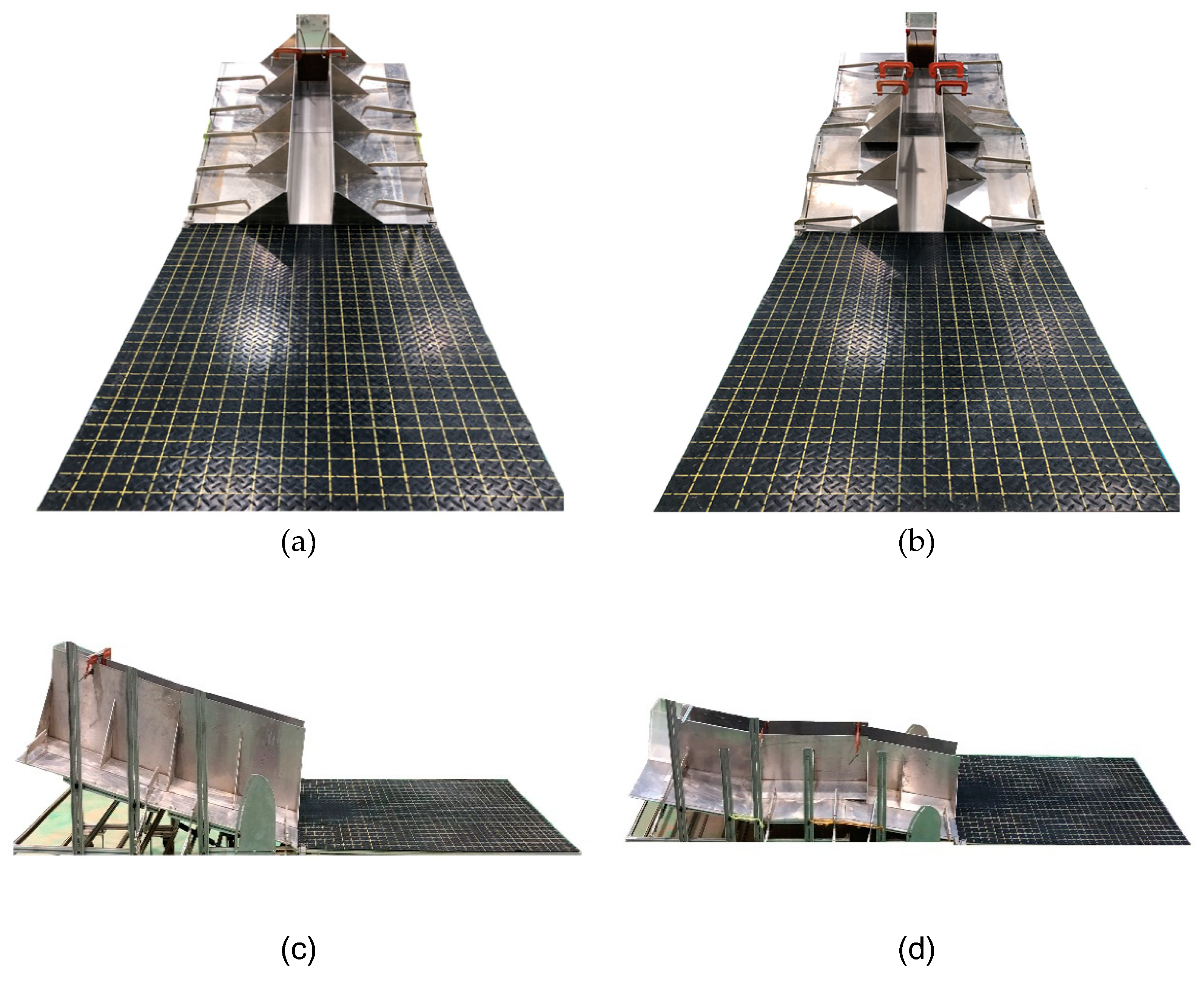
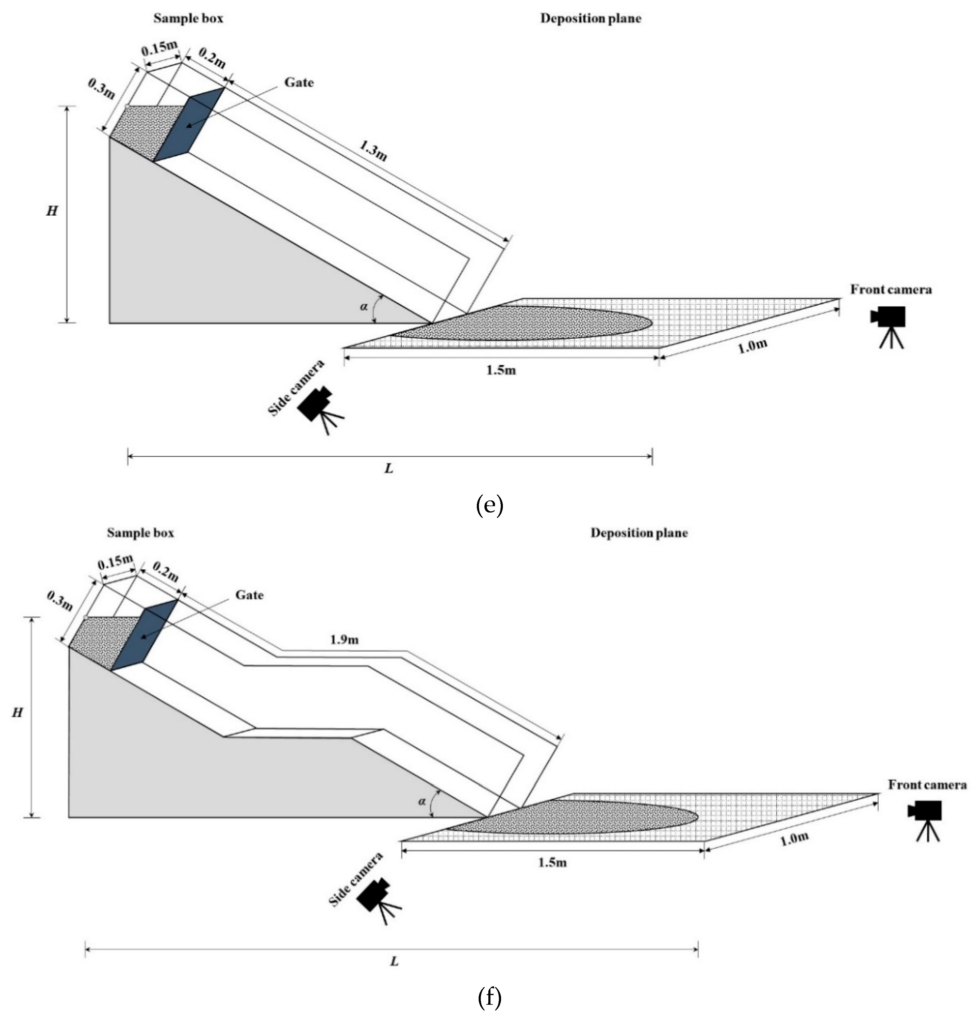
Figure 1. Examples of using berms in real world slopes: (a) Slopes with berms in coal mine areas (Dr Ajay Kumar Singh/Shutterstock.com); (b) slopes with berms in Peru (lialina/Shutterstock.com).
Applsci 11 02336 g001
Figure 2. Experimental setups for flume experiments: (a) Front image of the straight channel test; (b) front image of the single-berm channel test; (c) side image of the straight channel test; (d) side image of the single-berm channel test; (e) schematic diagram of the straight channel test; and (f) schematic diagram of the single-berm channel test.
Applsci 11 02336 g002aApplsci 11 02336 g002b
Figure 3. Grain-size distribution curve of the mixed sediment used in the debris flow.
Applsci 11 02336 g003
Figure 4. Examples of flume experiments conducted in this study: (a) Straight channel test (α was 25° and CV was 0.50); and (b) single-berm channel test (α was 25° and CV was 0.50).
Applsci 11 02336 g004
Figure 5. Flow chart of flume experiments.
Applsci 11 02336 g005
Figure 6. (a) Flow velocity according to α (at CV = 0.40–0.55); (b) flow velocity according to CV (at α = 10°–25°); (c) percent decrease in flow velocity due to berm according to α (at CV = 0.40–0.55); (d) percent decrease in flow velocity due to berm according to CV (at α = 10°–25°).
Applsci 11 02336 g006
Figure 7. (a) Flow depth according to α (at CV = 0.40–0.55); (b) flow depth according to CV (at α = 10°–25°); (c) percent decrease in flow depth due to berm according to α (at CV = 0.40–0.50); (d) percent decrease in flow depth due to berm according to CV (at α = 10°–25°).
Applsci 11 02336 g007
Figure 8. (a) Froude number according to α (at CV = 0.40–0.55); (b) Froude number according to CV (at α = 10°–25°); (c) percent increase in Froude number due to berm according to α (at CV = 0.40–0.50); (d) percent increase in Froude number due to berm according to CV (at α = 10°–25°).
Applsci 11 02336 g008
Figure 9. (a) μ according to α (at CV = 0.40–0.55); (b) μ according to CV (at α = 10°–25°); (c) ξ according to α (at CV = 0.40–0.55); (d) ξ according to CV (at α = 10°–25°); (e) n according to α (at CV = 0.40–0.55); (f) n according to CV (at α = 10°–25°); (g) C1 according to α (at CV = 0.40–0.55); (h) C1 according to CV (at α = 10°–25°); (i) C2 according to α (at CV = 0.40–0.55); (j) C2 according to CV (at α = 10°–25°).
Applsci 11 02336 g009aApplsci 11 02336 g009b
Figure 10. (a) Mobility ratio according to α (at CV = 0.40–0.55); (b) mobility ratio according to CV (at α = 10°–25°); (c) percent decrease in mobility ratio due to berm according to α (at CV = 0.40–0.55); (d) percent decrease in mobility ratio due to berm according to CV (at α = 10°–25°).
Applsci 11 02336 g010aApplsci 11 02336 g010b
Table 2. Dimensions of the channels for each test type.
Test TypeLength (m)Width (m)Height (m)
Straight channel test1.30.150.3
Single-berm channel test1.90.150.3
Table 3. Experimental conditions used in this study.
Straight Channel TestSingle-Berm Channel Test
Channel Slope α (°)1015202510152025
Volumetric
concentration CV
0.400.400.400.400.400.400.400.40
0.450.450.450.450.450.450.450.45
0.500.500.500.500.500.500.500.50
0.550.550.550.550.550.550.550.55
0.600.600.600.600.600.600.600.60
Table 4. Weight ratios of the sediment–water mixture by particle size.
Particle Size (mm)Weight Ratio (%)
4.750–9.50025.00
2.000–4.75025.00
0.850–2.00010.67
0.425–0.85020.63
0.250–0.42513.57
0.150–0.2503.63
0.075–0.1501.00
<0.0750.50
Table 5. Weight of debris flow samples according to volumetric concentration of sediment CV.
CV< 2 mm
(kgf)
2–4.75 mm
(kgf)
4.75–9.5 mm
(kgf)
Water (kgf)W
(kgf)
ρ
(kg·m−3)
0.402.2001.1001.1002.7007.1001578
0.452.4751.2381.2382.4757.4251650
0.502.7501.3751.3752.2507.7501722
0.553.0251.5131.5132.0258.0751794
0.603.3001.6501.6501.8008.4001867
Table 6. Observed data from flume experiments.
Test TypeNα (°)CVv (m·s−1)h (m)FrH (m)L (m)H/L
Straight channel1100.401.8260.01984.140.3912.4590.159
2100.451.6970.01604.280.3912.3400.167
3100.501.5590.01084.790.3912.1940.178
4100.551.3240.00585.550.3912.1050.186
5100.601.169--0.3911.7800.220
6150.401.9290.01844.540.5072.6300.193
7150.451.8110.01504.720.5072.5410.200
8150.501.6970.01045.310.5072.3390.217
9150.551.6210.00507.320.5072.0980.242
10150.601.2310.00386.380.5071.7630.288
11200.402.2650.01685.580.6202.6610.233
12200.452.0830.01425.580.6202.5600.242
13200.501.9120.01026.040.6202.4170.256
14200.551.8060.00488.320.6202.1760.285
15200.601.6290.00348.920.6201.7650.351
16250.402.4530.01546.310.7282.7390.266
17250.452.3470.01047.350.7282.6130.278
18250.502.1810.00947.180.7282.4290.300
19250.552.0700.00459.850.7282.1870.333
20250.601.9120.003210.790.7281.8170.400
Single-berm channel21100.401.5940.01254.550.3912.9070.134
22100.451.3830.00794.970.3912.5870.151
23100.501.152--0.3912.3490.166
24100.550.870--0.3912.2550.173
25100.60------
26150.401.7460.01065.410.5072.9690.171
27150.451.5270.00785.520.5072.7910.182
28150.501.4350.00308.360.5072.6020.195
29150.551.153--0.5072.2520.225
30150.60------
31200.402.0260.01046.340.6203.0890.201
32200.451.8550.00746.880.6202.8730.216
33200.501.6780.00547.290.6202.6170.237
34200.551.319--0.6202.2800.272
35200.60------
36250.402.3750.01785.680.7283.1590.230
37250.452.1840.01006.970.7282.9380.248
38250.501.9670.00807.020.7282.6470.275
39250.551.6990.00309.900.7282.3800.306
40250.60------
Table 7. Flow resistance coefficients calculated in this study.
Flow Resistance CoefficientRangeMeanStandard Deviation
μ (Pa·s)0.006–0.2430.0890.075
ξ (m−1/2·s−1)2240–30,76491527514
n (m−1/3·s)0.006–0.0190.0120.003
C1 (m1/2·s−1)27.47–61.5338.878.132
C2 (m0.78·s−1)6.48–9.058.000.639
Publisher’s Note: MDPI stays neutral with regard to jurisdictional claims in published maps and institutional affiliations.

